Determining the Age of Terrace Formation Using Luminescence Dating-A Case of the Yellow River Terraces in the Baode Area, China - MDPI
←
→
Page content transcription
If your browser does not render page correctly, please read the page content below
Protocol
Determining the Age of Terrace Formation Using
Luminescence Dating—A Case of the Yellow River
Terraces in the Baode Area, China
Jia-Fu Zhang 1, * , Wei-Li Qiu 2 , Gang Hu 1,3 and Li-Ping Zhou 1
 1   MOE Laboratory for Earth Surface Processes, College of Urban and Environmental Sciences,
     Peking University, Beijing 100871, China; hugang@ies.ac.cn (G.H.); lpzhou@pku.edu.cn (L.-P.Z.)
 2   Faculty of Geographical Science, Beijing Normal University, Beijing 100875, China; qiuweili@bnu.edu.cn
 3   Institute of Geology, China Earthquake Administration, Beijing 100029, China
 *   Correspondence: jfzhang@pku.edu.cn

 Received: 12 November 2019; Accepted: 17 February 2020; Published: 20 February 2020

 Abstract: Dating fluvial terraces has long been a challenge for geologists and geomorphologists,
 because terrace straths and treads are not usually directly dated. In this study, the formation ages
 of the Yellow River terraces in the Baode area in China were determined by dating fluvial deposits
 overlying bedrock straths using optically stimulated luminescence (OSL) dating techniques. Seven
 terraces (from the lowest terrace T1 to the highest terrace T7) in the study area were recognized, and
 they are characterized by thick fluvial terrace deposits overlaid by loess sediments. Twenty-five
 samples from nine terrace sections were dated to about 2–200 ka. The OSL ages (120–190 ka) of
 the fluvial samples from higher terraces (T3–T6) seem to be reliable based on their luminescence
 properties and stratigraphic consistency, but the geomorphologic and stratigraphic evidence show
 that these ages should be underestimated, because they are generally similar to those of the samples
 from the lower terrace (T2). The formation ages of the terrace straths and treads for the T1 terrace
 were deduced to be about 44 ka and 36 ka, respectively, based on the deposition rates of the fluvial
 terrace deposits, and the T2 terrace has the same strath and tread formation age of about 135 ka. The
 incision rate was calculated to be about 0.35 mm/ka for the past 135 ka, and the uplift rate pattern
 suggests that the Ordos Plateau behaves as a rigid block. Based on our previous investigations
 on the Yellow River terraces and the results in this study, we consider that the formation ages of
 terrace straths and treads calculated using deposition rates of terrace fluvial sediments can overcome
 problems associated with age underestimation or overestimation of strath or fill terraces based on
 the single age of one fluvial terrace sample. The implication is that, for accurate dating of terrace
 formation, terrace sections should be systematically sampled and dated.

 Keywords: terrace strath and tread ages; luminescence dating; deposition rate; age-depth model;
 Yellow River terrace

1. Introduction
     Fluvial terrace deposits and landforms can provide important information about river incision,
tectonic activity, climate change and archaeological traces of hominid activity [1–5], and terraces record
different stages of fluvial evolution and sedimentation. Yet, understanding the formation of terraces is a
perennial problem in geomorphology and has been hampered by the exact timing of terrace formation.
Determining the formation age of terraces is a challenge for geomorphologists and geologists. Recently,
the successful application of optically stimulated luminescence (OSL) dating techniques [6–8] to fluvial
sediments [9,10] has made it possible to establish the chronology of terraces by dating fluvial sediments
atop terrace straths [11–15]. Conventionally, only a single age is assigned to a terrace, but this may

Methods Protoc. 2020, 3, 17; doi:10.3390/mps3010017                                 www.mdpi.com/journal/mps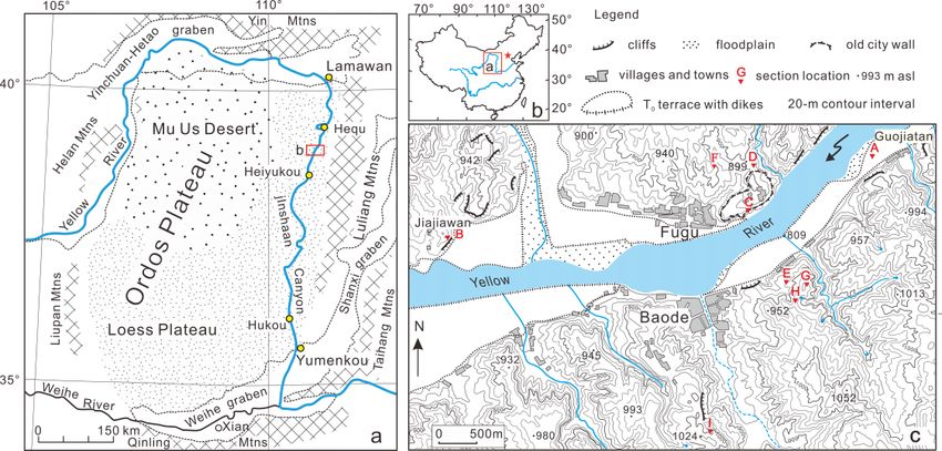
Methods Protoc. 2020, 3, 17                                                                          2 of 20

not reflect actual fluvial processes [16,17]. The development of OSL techniques allows dating a series
of samples from terrace deposits by systematic sampling, which helps to establish the chronology of
deposition and then deduce the formation ages of terrace straths and treads [18–20].
      The investigations of Yellow River fluvial terraces have become one of the most important topics
in Chinese geomorphology and are also of interest to researchers in sedimentology, engineering,
hydrology and archaeology. The fluvial terraces in the Jinshaan Canyon in the middle reaches of the
Yellow River have been widely investigated and dated mainly using luminescence and paleomagnetic
dating methods [18,19,21–26]. However, the dates of the terraces obtained are not enough to construct
the precise chronology of a series of terraces in the region. This is further complicated by the fact
that some terraces with the same elevations above the modern river have different formation ages,
because their formations are controlled by knickpoint migration [19,25]. Therefore, it is necessary to
determine the ages of more Yellow River terraces in different localities of the region. On the other hand,
one sample for OSL dating is often collected from terrace deposits in fluvial terrace investigations [21],
and its age is usually assumed to be the terrace formation age. This assumption may be incorrect, and
its validity needs to be tested. In this study, we first identified terraces in the two banks of the Yellow
River in the Baode area in the middle reaches of the river, and terrace deposits were systematically
sampled for OSL dating, i.e., a series of samples were collected from channel facies and floodplain
facies and overlying loess deposits on terraces. The reliability of their ages was evaluated based on the
internal consistency of the OSL ages and the lithostratigraphic and geomorphological consistency in
the OSL ages, and the formation ages of terrace straths and treads were then inferred.

2. Geological and Geomorphologic Setting
     The Ordos Plateau, with an area of 320,000 km2 located in the western part of the North China
block, is a relatively stable rigid block (Figure 1a) [27,28]. It is bounded by a series of marginal faults
and orogenic belts [29–34]. The basement of the plateau is composed of Archean and Proterozoic
metamorphic rocks that are overlain by Cambrian and Ordovician marine carbonates with the lack
of Silurian and Devonian strata. Carboniferous marine limestone and fluvial-deltaic sandstone are
overlain by fluvial Permian strata. Triassic and Jurassic strata are composed of fluvial and lacustrine
deposits, which are overlain by Cretaceous fluvial and eolian redbeds. The Ordos block evolved from
a basin to a plateau during the late Miocene–Pliocene, which influences the environmental effect on
the topography of the area [35]. Geomorphologically, the Ordos Plateau is surrounded by the Yin
Mountains to the north, Luliang Mountains to the east, Qinling Mountains to the south, Liupan and
Helan Mountains to the west (Figure 1). The arc-shaped Yinchuan–Hetao graben system along the
northwestern and northern margins of the block and the S-shaped Weihe-Shanxi graben system along
the southeastern margins bound the plateau [29,36]. The plateau is covered by Quaternary eolian
sediments. The northern part, the Mu Us Desert, is mantled by dune sands, and the southern part, the
Chinese Loess Plateau, is covered by loess/paleosol deposits.
     The Yellow River (called Huanghe in Chinese), well-known for its tremendous sediment load,
originates in the northeast of the Tibetan Plateau. In its middle reaches, the river flows along the
northeastern and northern margins of the Ordos Plateau and cuts through the eastern plateau at an
average elevation ranging from 1000 to 1500 m above sea level (asl), from Lamawan in the north to
Yumenkou in the south (Figure 1a). The river then turns east and finally overflows into the Bohai Sea.
The river downcutting between Lamawan and Yumenkou leads to the formation of a deep and narrow
gorge called Jinshaan Canyon, which connects the Yinchuan-Hetao graben on the north and the Weihe
graben on the south. A series of strath terraces along the banks of the canyon have been found based
on the presence of fluvial deposits and bedrock strath. The terrace treads are covered by loess with
various thicknesses.
Methods Protoc. 2020, 3, 17 3 of 20
Methods Protoc. 2020, 3, x FOR PEER REVIEW 3 of 21
Figure1.1. (a,b)
Figure (a,b)Map
Mapshowing
showingthetheYellow
Yellow River
River course
course along
along thethe margins
margins of the
of the OrdosOrdos Plateau
Plateau and
and location
location of the of the area
study study area (Baode);
(Baode); (c) topographic
(c) topographic map showingmap theshowing
localitiesthe localities
of the sectionsof(A–I)
the
sections
shown in (A–I)
Figureshown in Figure 2.map
2. The topographic The with
topographic map with
contour intervals contour
of 20 m was intervals
constructedof based
20 m onwasa
constructed
Chinese based
1:50,000 on a Chinese
topographic 1:50,000 topographic map (unpublished).
map (unpublished).
3.
3. Methodology
Methodology
3.1. Field Work
3.1. Field Work
As shown in Figure 1a, the two banks of the Yellow River in the study area are covered by
As shown in Figure 1a, the two banks of the Yellow River in the study area are covered by
loess/paleosol deposits. This implies that the original stair-stepped topography of the fluvial terraces
loess/paleosol deposits. This implies that the original stair-stepped topography of the fluvial terraces
in the area is not directly observed, and the situation is further complicated by the modification of the
in the area is not directly observed, and the situation is further complicated by the modification of
loess landscape due to soil erosion. The fluvial terraces cannot be mapped from topographic maps,
the loess landscape due to soil erosion. The fluvial terraces cannot be mapped from topographic
satellite images or air photos or even identified in the field based on surface landform. In this case, the
maps, satellite images or air photos or even identified in the field based on surface landform. In this
identification of remnants of the terraces was only conducted by observing fluvial sediments exposed
case, the identification of remnants of the terraces was only conducted by observing fluvial sediments
in natural outcrops or road-cuts in the field. This means that the terraces were found as isolated
exposed in natural outcrops or road-cuts in the field. This means that the terraces were found as
remnants. The heights of terrace strath (bedrock surface) and tread (here the “tread” is referred to as
isolated remnants. The heights of terrace strath (bedrock surface) and tread (here the “tread” is
the near-horizontal top surface of fluvial deposits, including channel or overbank facies resting on
referred to as the near-horizontal top surface of fluvial deposits, including channel or overbank facies
terrace straths) above the modern river level and the thickness of the terrace deposits were measured
resting on terrace straths) above the modern river level and the thickness of the terrace deposits were
using a total station and a tape measure. The precise locations and altitude of the exposures were
measured using a total station and a tape measure. The precise locations and altitude of the exposures
recorded using a hand-held global positioning system (GPS) receiver with a barometric altimeter
were recorded using a hand-held global positioning system (GPS) receiver with a barometric
(Garmin GPSmap 60CSx) with an accuracy of ±~3 m in altitude. Stratigraphy and lithology of the
altimeter (Garmin GPSmap 60CSx) with an accuracy of ±~3 m in altitude. Stratigraphy and lithology
exposures were described in detail.
of the exposures were described in detail.
A systematic sampling strategy was adopted for dating the sediments on terrace straths using
A systematic sampling strategy was adopted for dating the sediments on terrace straths using
OSL techniques. Systematic sampling means that a series of samples are taken from fluvial and loess
OSL techniques. Systematic sampling means that a series of samples are taken from fluvial and loess
deposits on a terrace, and their OSL ages are used to construct an age-depth model for the terrace
deposits on a terrace, and their OSL ages are used to construct an age-depth model for the terrace
deposits. The model helps us to evaluate the reliability of OSL ages obtained for the terraces and to
deposits. The model helps us to evaluate the reliability of OSL ages obtained for the terraces and to
explain the history of river incision. The formation ages of the strath and tread for a terrace can be
explain the history of river incision. The formation ages of the strath and tread for a terrace can be
inferred from the age-depth relationship. OSL samples were taken from each unit of terrace deposits
inferred from the age-depth relationship. OSL samples were taken from each unit of terrace deposits
and overlying loess/paleosol (see Figure 2). The samples were collected by hammering 3.5-cm-diameter
and overlying loess/paleosol (see Figure 2). The samples were collected by hammering 3.5-cm-
and 30-cm-long stainless-steel tubes horizontally into freshly cleaned exposures. The tubes were
diameter and 30-cm-long stainless-steel tubes horizontally into freshly cleaned exposures. The tubes
wrapped with aluminum foil and adhesive tape in order to prevent further exposure to light and
were wrapped with aluminum foil and adhesive tape in order to prevent further exposure to light
moisture loss.
and moisture loss.Methods Protoc. 2020, 3, 17 4 of 20
Methods Protoc. 2020, 3, x FOR PEER REVIEW 4 of 21
Figure 2. Stratigraphic
Figure columns
2. Stratigraphic of theofterrace
columns deposits
the terrace in outcrops
deposits (A–I) marked
in outcrops in Figurein1c,
(A–I) marked and the
Figure
positions
1c, andofthe
optically stimulated
positions luminescence
of optically stimulated (OSL) samples and
luminescence ages samples
(OSL) in ka. Theand
elevations
ages in of
ka.bedrock
The
surfaces (strath
elevations ofsurface)
bedrockabove the modern
surfaces river areabove
(strath surface) displayed.
the modern river are displayed.
3.2. Optical Dating
3.2. Optical Dating
3.2.1. Equivalent Dose Measurements
3.2.1. Equivalent Dose Measurements
The samples for OSL measurements were prepared in our dark room with a dim red light at
The samples for OSL measurements were prepared in our dark room with a dim red light at the
thePeking
PekingUniversity,
University, Beijing,
Beijing, China.
China. Coarse-
Coarse- and and fine-grained
fine-grained quartzquartz were extracted
were extracted from sand-fromand sand-
and silt-sized samples using the procedures in our laboratory, respectively
silt-sized samples using the procedures in our laboratory, respectively [37,38]. In the laboratory, the[37,38]. In the laboratory,
thelight-exposed
light-exposed ends
ends (about
(about 2–3ofcm
2–3 cm of sediment)
sediment) of a sample
of a sample tube were tubefirstwere
removed,first and
removed, and this
this removed
removed
material was used for dose-rate analysis. The remaining material from the middle of the tubethe
material was used for dose-rate analysis. The remaining material from the middle of wastube
was treated
treated with
with 10%10% hydrochloric
hydrochloric acid
acid to to dissolve
dissolve carbonates
carbonates andandthen then 30%
30% hydrogen
hydrogen peroxide
peroxide to to
remove
remove organic
organicmaterial,
material,respectively.
respectively. For
For sand-sized samples,the
sand-sized samples, thematerial
materialwas wasthen
then washed
washed with
with
water
water to to
eliminate
eliminatefiner
finergrains, followedby
grains, followed bydrying
dryingand and sieving
sieving to select
to select coarsecoarse grains
grains (grain(grain sizes
sizes for
foreach
eachsample
sampleare listed
are listedin in
Table 1) for
Table luminescence
1) for luminescence measurements.
measurements. The coarse-grained
The coarse-grained quartz quartz
was
wasobtained
obtained by by
immersing
immersing the sieved sample
the sieved in 40%inHF
sample 40%forHF40 or
for8040min or and
80 minthenand10%then
HCl to 10% remove
HCl to
feldspar
remove contaminants.
feldspar For fine-grained
contaminants. samples,samples,
For fine-grained the samples the were
samplesthenwere deflocculated using a dilute
then deflocculated using
sodium oxalate solution, and polymineral fine grains (4–11 μm) were
a dilute sodium oxalate solution, and polymineral fine grains (4–11 µm) were isolated by settling isolated by settling the
polymineral fine silt fraction in the solution. Fine-grained quartz
the polymineral fine silt fraction in the solution. Fine-grained quartz was obtained by treatingwas obtained by treating thethe
polymineral
polymineral extracts
extracts withsilica-saturated
with silica-saturatedfluorosilicic
fluorosilicic acidacid (H
(H22SiF
SiF6)6 )atatroom
roomtemperature
temperature to to
dissolve
dissolve
feldspars, amorphous silica and other contaminant minerals, followed
feldspars, amorphous silica and other contaminant minerals, followed by a treatment with 10% HCl by a treatment with 10% HCl to
to remove any fluorides produced. The purity of the quartz extracts was checked by infrared
remove any fluorides produced. The purity of the quartz extracts was checked by infrared stimulation.
stimulation. The results showed that the infrared-stimulated luminescence signals were negligible,
The results showed that the infrared-stimulated luminescence signals were negligible, indicating
indicating feldspar contaminants were almost entirely removed. The chemically purified quartz was
feldspar contaminants were almost entirely removed. The chemically purified quartz was prepared for
prepared for luminescence measurements by settling the fine grains in acetone onto 0.97-cm-diameter
luminescence measurements by settling the fine grains in acetone onto 0.97-cm-diameter aluminum
aluminum discs or mounting the coarse grains as a monolayer on 0.97-cm-diameter aluminum discs
discs or mounting the coarse grains as a monolayer on 0.97-cm-diameter aluminum discs with the
with the grains covering the area with a diameter of ~5 mm (medium aliquots) using silicone oil as
grains covering the area with a diameter of ~5 mm (medium aliquots) using silicone oil as an adhesive.
an adhesive.
The improved single-aliquot regenerative dose procedure (SAR) [39,40] was used to measure
the single-aliquot equivalent dose (De) of the quartz extracts at Peking University. The regenerative
beta doses used in the SAR procedure included a zero dose used for monitoring recuperation effects
and a repeat of the first regeneration dose used to check the reproducibility of the sensitivity
correction (i.e., recycling ratio). Based on the results of the preheat plateau and dose recovery tests
(see below), the preheat temperature was set to 220 °C or 260 °C, and the cut-heat temperature to 160
°C. OSL signals were measured for 40 s at 125 °C. In addition, a 20-s IR stimulation at roomMethods Protoc. 2020, 3, 17 5 of 20
Table 1. The results of optical dating of the samples from the Yellow River terraces in the Baode area.
Water No. of Arithmetic Central Age Modeling (CAM)
Section Depth Grain Dose rate
No. Lab Code Field No. (m) Sediment Size (µm) K * (%) K ** (%) U ** (ppm) Th ** (ppm) Content
(Gy/ka) Aliquots Mean De OD+ Mean De
# (%)
Measured (Gy) Age (ka)
(%) (Gy)
Terrace T0
Overbank
A L552 BD-OSL06 0.98 4–11 1.8 1.87 ± 0.10 2.36 ± 0.10 9.81±0.24 10 3.30 ± 0.12 3 30.4 ± 1.1 30.5 ± 1.2 9.2 ± 0.5
silt
Channel
L551 BD-OSL05 2.05 90–125 1.72 1.63 ± 0.09 2.02 ± 0.09 10.10 ± 0.22 5 2.89 ± 0.08 21 6.7 ± 1.5 72 5.0 ± 0.8 1.7 ± 0.3
sand
Channel
L550 BD-OSL04 3.30 150–250 2.98 3.25 ± 0.11 0.68 ± 0.06 5.52 ± 0.17 5 3.69 ± 0.10 25 13.5 ± 2.4 69 10.0 ± 1.5 2.7 ± 0.4
sand
Channel
L549 BD-OSL03 4.77 150–250 2.35 2.32 ± 0.10 0.83 ± 0.07 5.63 ± 0.16 5 2.84 ± 0.09 21 53.7 ± 5.5 53 47.4 ± 5.6 16.7 ± 2.0
sand
Terrace T1
B L784 BD06-OSL03 2.40 Loess 4–11 1.4 3.01 ± 0.37 11.41 ± 1.24 10 3.12 ± 0.15 4 91.3 ± 5.4 90.7 ± 4.8 29.1 ± 2.1
Channel
L783 BD06-OSL02 8.80 150–250 1.85 2.48 ± 0.33 9.13 ± 1.10 * 5 2.95 ± 0.11 21 122.7 ± 7.2 22 117.6 ± 6.0 39.8 ± 2.5
sand
Channel
L782 BD06-OSL01 11.20 150–250 1.65 2.01 ± 0.37 12.24 ± 1.24 * 5 2.85 ± 0.11 21 125.2 ± 7.2 21 119.5 ± 6.3 41.9 ± 2.7
sand
Terrace T2
Overbank
C L567 BD-OSL21 1.05 90–125 1.72 1.68 ± 0.10 1.59 ± 0.07 8.75 ± 0.22 10 2.64 ± 0.09 16(2) 378.9 ± 65.8 21 357 ± 24 135 ± 10
silt
Overbank
L568 BD-OSL22 2.00 90–125 1.72 1.64 ± 0.10 1.90 ± 0.09 8.02 ± 0.20 10 2.60 ± 0.09 13 369.4 ± 17.6 12 355 ± 18 137 ± 8
silt
Overbank
L569 BD-OSL23 2.70 90–125 1.72 1.72 ± 0.10 1.80 ± 0.08 7.32 ± 0.20 10 2.59 ± 0.09 8 366.0 ± 41.8 29 346 ± 38 134 ± 15
silt
Terrace T3
Channel
D L571 BD-OSL25 4.8 150–250 2.2 2.35 ± 0.09 1.09 ± 0.08 6.49 ± 0.18 5 2.98 ± 0.08 20 366.9 ± 14.5 13 365 ± 13 122 ± 6
sand
Channel
L570 BD-OSL24 9.8 90–150 1.88 1.09 1.70 ± 0.10 8.62 ± 0.21 5 2.73 ± 0.09 22 361.8 ± 25.5 29 344 ± 23 126 ± 9
sand
Terrace T4
Channel
E L557 BD-OSL11 4.80 125–150 1.8 1.80 ± 0.09 1.23 ± 0.07 5.83 ± 0.17 5 2.50 ± 0.08 23 357.3 ± 21.0 23 339 ± 15 135 ± 7
sand
Channel
L556 BD-OSL10 16.2 150–250 2.2 2.10 ± 0.09 0.80 ± 0.07 5.03 ± 0.16 5 2.51 ± 0.08 23 321.1 ± 20.3 26 310 ± 18 123 ± 8
sand
Terrace T5Methods Protoc. 2020, 3, 17 6 of 20
Table 1. Cont.
Water No. of Arithmetic Central Age Modeling (CAM)
Section Depth Grain Dose rate
No. Lab Code Field No. (m) Sediment Size (µm) K * (%) K ** (%) U ** (ppm) Th ** (ppm) Content
(Gy/ka) Aliquots Mean De OD+ Mean De
# (%)
Measured (Gy) Age (ka)
(%) (Gy)
F L787 BD06-OSL06 12.9 Loess 4–11 1.95 2.62 ± 0.40 13.19 ± 1.33 * 10 3.55 ± 0.17 4 228.3 ± 3.2 228.9 ± 6.6 65 ± 4
Overbank
L786 BD06-OSL05 16.00 4–11 1.65 2.01 ± 0.35 10.89 ± 1.18 * 10 2.93 ± 0.14 3 578.0 ± 20.4 570 ± 23 195 ± 12
silty clay
Overbank
L785 BD06-OSL04 22.20 4–11 1.65 2.37 ± 0.35 10.72 ± 1.18 * 10 2.99 ± 0.14 4 590.1 ± 53.6 559 ± 26 187 ± 12
silty clay
Channel
L573 BD-OSL27 23.00 90–125 2.67 2.69 ± 0.10 1.00 ± 0.08 6.42 ± 0.18 5 3.27 ± 0.09 52 481.9 ± 20.6 24 456 ± 19 139 ± 7
sand
Channel
L572 BD-OSL26 25.7.00 90–125 2.35 2.45 ± 0.09 1.18 ± 0.08 11.50 ± 0.25 5 3.43 ± 0.08 25 509.3 ± 35.3 23 476 ± 26 139 ± 8
sand
Terrace T6
G L559 BD-OSL13 3.10 Loess 4–11 1.72 1.78 ± 0.09 2.57 ± 0.09 9.67 ± 0.22 10 3.21 ± 0.12 5 612.8 ± 25.0 607 ± 32 189 ± 12
L558 BD-OSL12 7.00 Paleosol 4–11 1.96 2.07 ± 0.09 2.07 ± 0.09 11.50 ± 0.25 15 3.26 ± 0.12 5 642.9 ± 38.0 609 ± 17 187 ± 8
H L564 BD-OSL18 1.00 Loess 4–11 1.88 1.73 ± 0.10 1.88 ± 0.09 9.15 ± 0.22 10 3.00 ± 0.12 6 593.1 ± 37.1 571 ± 29 191 ± 12
L563 BD-OSL17 5.15 Paleosol 4–11 2.04 2.23 ± 0.10 2.00 ± 0.08 9.60 ± 0.22 15 3.27 ± 0.12 6 605.1 ± 20.3 623 ± 24 191 ± 10
Channel
L562 BD-OSL16 7.10 150–250 2.2 2.32 ± 0.09 0.96 ± 0.07 5.64 ± 0.16 5 2.84 ± 0.08 21 547.0 ± 28.4 23 531 ± 29 187 ± 12
sand
Channel
L561 BD-OSL15 9.10 150–250 2.2 2.10 ± 0.09 0.80 ± 0.07 4.39 ± 0.15 5 2.50 ± 0.08 25 497.6 ± 32.2 31 474 ± 31 190 ± 15
sand
*: Determined using flame photometry; **: Determined using neutron-activation-analysis (NAA), except for samples L782–787, for these six samples whose U and Th contents were
determined using the alpha counting method; the K contents obtained using NAA were used for dose rate calculation, except for samples L782–787 (for these six samples, the K contents
obtained using flame photometry were used, and a relative uncertainty of 5% was assumed); OSL: optically stimulated luminescence; # : Relative uncertainty of 20% is assumed for water
contents for all samples; + : OD = overdispersion; for fine grains, the OD value is not calculated. All uncertainties are reported as one sigma.Methods Protoc. 2020, 3, 17 7 of 20
The improved single-aliquot regenerative dose procedure (SAR) [39,40] was used to measure the
single-aliquot equivalent dose (De) of the quartz extracts at Peking University. The regenerative beta
doses used in the SAR procedure included a zero dose used for monitoring recuperation effects and
a repeat of the first regeneration dose used to check the reproducibility of the sensitivity correction
(i.e., recycling ratio). Based on the results of the preheat plateau and dose recovery tests (see below),
the preheat temperature was set to 220 ◦ C or 260 ◦ C, and the cut-heat temperature to 160 ◦ C. OSL
signals were measured for 40 s at 125 ◦ C. In addition, a 20-s IR stimulation at room temperature before
each OSL measurement was carried out to remove the possible effect of feldspar contamination [38],
although IRSL signals were negligible, and a 40-s blue light stimulation at 280 ◦ C at the end of each
cycle was also carried out for reducing recuperation. The signals were analyzed using late background
subtraction (the intensity of the initial 0.16 s minus a background (normalized to 0.16 s) from the last
3.2 s), and the value of De was estimated by interpolating the sensitivity-corrected natural OSL onto the
dose-response curve using the Analyst software [41]. The error on individual De values was calculated
using the counting statistics and an instrumental uncertainty of 1.0%.
All luminescence measurements, beta irradiation and preheat treatments were carried out in
automated Risø TL/OSL (DA-15 and DA-20) readers equipped with a 90 Sr/90 Y beta source (the Risoe
National Laboratory, Denmark Technical University, Denmark) [42]. Blue light LED (470 ± 30 nm)
stimulation was used for quartz OSL measurements and an IR laser diode (830 ± 10 nm) stimulation
for scanning feldspar contamination and for feldspar IRSL measurements. Luminescence was detected
by an EMI 9235QA photomultiplier tube with two Hoya U-340 filters (290–370 nm) in front of it.
3.2.2. Dose Rate Determination
The uranium and thorium contents of samples L782–787 were determined using thick-source alpha
counting (a Littlemore low-level alpha counter 7286 with 42-mm-diameter ZnS screens) (Littlemore
Scientific, UK), and other samples were analyzed using the neutron-activation-analysis (NAA) for U,
Th and K contents. The K content of all samples was also measured using flame photometry.
The present-day water contents (ratio of mass of water/dry-sample [6]) of all the samples were
measured in the laboratory to be 1.0%–8.4%, with an average of 3.1±0.5%, by weight. These samples
were taken from the subsurface position of the sections, and they have been partly dried due to
exposure to air before sampling. These values are clearly not to be representative of the long-term
water contents in the natural conditions during most of the burial history. In this case, the water
contents used for dose rate calculation were assumed and taken as 5% for sand, 10% for loess and
silt sediments (overbank deposits) and 15% for paleosol. A relative uncertainty is taken as 20% to the
long-term water content values. This large uncertainty on the water content should cover the water
content fluctuations during burial. An alpha efficiency factor (a-value) of 0.038 ± 0.003 for quartz [43]
was used to calculate the alpha contribution to the total dose rate. Based on the above measurements,
the effective dose rates and ages were calculated using the online dose rate and age calculator DRAC
v1.2 [44], in which cosmic ray contribution and conversion factors [45] are involved, and the alpha [46]
and beta [47] grain attenuation factors were used.
4. Results
4.1. Terraces and Deposits
A total of nine exposures of fluvial sediments in the study area were found and observed.
Their locations (numbered A to I) are marked in Figure 1c, and their detailed lithology are shown in
Figure 2. It can be seen that the sections (exposures) are mainly composed of fluvial sediments called
terrace deposits and overlying eolian sediments. The fluvial sediments consist of channel gravels
and sands capping the strath surfaces and overbank silt or silty clay overlying the channel deposits.
The top eolian layers composed of loess, paleosol or red clay were deposited after paleo-floodplains
were completely abandoned. The bedrock surfaces (strath) of Sections B–I were presented, and theirMethods Protoc. 2020, 3, 17 8 of 20
elevations range from about 13 m to 176 m above the modern river level (arl) (Figure 2). Based on
the elevation of the straths, Exposures B–I are considered to represent seven terraces, from the lowest
T1 terrace with the elevation of about 13 m arl and the highest T7 terrace with the elevation of 176
m arl. Accordingly, a schematic composite across-section of the terraces was generated based on the
elevations of the terraces and their spatial distribution and is shown in Figure 3. Note that T0 (Section
A) is referred to the high floodplain of the river. Exposures (Sections) G and H have the same elevation
of strath (111 m arl) and belong to the T6 terrace. It is noted that the effect of the variations in river
gradients on terrace height in the study area is negligible.
The high floodplain (T0) is composed of sand interbedded with gravel and laminated silty
(Figure 2A), and the thickness of the fluvial deposits is more than 4.5 m. The top layer of this section
was disturbed by human activities. The thickness of the terrace deposits, including channel facies
(gravels and sands) and overbank facies (silts), for the eight sections ranges from ~10 to ~16 m.
The fluvial gravels have moderate-to-high sphericity and are well-rounded. The gravel layers have a
thickness ranging from 1 to 12 m, within which, crude imbrication is present locally, such as in Section
G. The overbank silts overlying gravel layers are characterized by thin horizontal bedding. Some silty
layers are interbedded with sand or gravel or sand lenses. The thickness of the silt layers varies from 0
to 8 m. The top loess/paleosol deposits are characterized by massive structure and vertical joints. On
the highest terrace (T7, Section I), the red clay deposits were found between the top loess and fluvial
sandy gravels resting on the bedrock. It is noted that the pre-Quaternary red clay deposits [48,49] are
far beyond the upper limit of luminescence dating. Therefore, the T7 terrace is not sampled for OSL
dating. The bedrock mainly comprises Triassic sandstone with a horizontal bedding, and the surface
Methods Protoc. 2020, 3, x FOR PEER REVIEW
of bedrock is loose because of weathering. As shown in Figure 2, a total of 25 samples for9OSL of 21
dating
were taken
dating were taken from sections A to H. The information about the samples are listed in Table 1, and their
from sections A to H. The information about the samples are listed in Table 1, and
positions arepositions
their also shown are alsoin shown
Figurein2.Figure 2.
Figure 3. Schematic
Figure composite
3. Schematic cross-section
composite across across
cross-section the Jinshaan Canyon
the Jinshaan at theat
Canyon Baode area showing
the Baode area the
showing
Yellow River the sequence
terrace Yellow River terrace and
and fluvial sequence and loess/paleosol
overlying fluvial and overlying
deposits,loess/paleosol
which are shown in
deposits,
details in Figure 2which
(here,are
theshown
lettersinrefer
details in number
to the Figure 2 of
(here, the letters
sections refer2).
in Figure to the number of
sections in Figure 2).
4.2. OSL Ages
4.2. OSL Ages
Two dose-response curves (DRC) and two typical OSL decay curves for a fine quartz aliquot from
Two dose-response curves (DRC) and two typical OSL decay curves for a fine quartz aliquot
a loess sample from the T6 terrace and a coarse quartz aliquot from a fluvial sample from the T5 terrace
from a loess sample from the T6 terrace and a coarse quartz aliquot from a fluvial sample from the
are shown in Figure
T5 terrace 4. Theindecay
are shown Figure curves demonstrate
4. The decay that the that
curves demonstrate quartz OSL signals
the quartz are are
OSL signals easily bleached
easily
and dominated
bleached by
andfast components.
dominated The dose response
by fast components. curves are
The dose response well-fitted
curves with with
are well-fitted a double-saturating
a double-
exponential function
saturating or a saturating
exponential function orexponential plus linearplus
a saturating exponential function. The recycling
linear function. ratiosratios
The recycling are close to
are close to unity, and the recuperation values are less than 0.5%. The DRCs
unity, and the recuperation values are less than 0.5%. The DRCs for all the samples are very for all the samples are similar,
very similar, and the natural signals are apparently not close to saturation.
and the natural signals are apparently not close to saturation.
Preheat plateau and dose recovery tests were carried out on two samples to find the most
Preheat plateau and dose recovery tests were carried out on two samples to find the most suitable
suitable preheat temperature in the SAR procedure for our samples. Preheat plateau tests were
preheat performed
temperature in the
using theSAR
SARprocedure
procedure fordifferent
with our samples.
preheat Preheat plateau
temperatures testsfrom
ranging were160performed
°C to 300 using
°C at an interval of 20 °C. The results shown in Figure 5 demonstrate that the De values are
independent of preheat temperatures, at least between 220 °C and 280 °C, for both samples. Dose
recovery tests were performed on the same samples to further confirm the results of the preheat
plateau tests. After removing the natural OSL signals by exposing aliquots to blue light within the
readers at room temperature for 40 s, the residual OSL signals were examined by a second 40-s OSL
measurement ~10,000 s after bleaching, and no detectable OSL signals could be observed. TheMethods Protoc. 2020, 3, 17 9 of 20
the SAR procedure with different preheat temperatures ranging from 160 ◦ C to 300 ◦ C at an interval
of 20 ◦ C. The results shown in Figure 5 demonstrate that the De values are independent of preheat
temperatures, at least between 220 ◦ C and 280 ◦ C, for both samples. Dose recovery tests were performed
on the same samples to further confirm the results of the preheat plateau tests. After removing the
natural OSL signals by exposing aliquots to blue light within the readers at room temperature for 40 s,
the residual OSL signals were examined by a second 40-s OSL measurement ~10,000 s after bleaching,
and no detectable OSL signals could be observed. The aliquots were then irradiated with a laboratory
beta dose approximately equal to the natural dose (De) of the sample. This artificial dose (given dose)
was then taken as unknown, and the aliquots were treated as “natural samples”. After a storage of
at least 10 h, the irradiated aliquots were then measured using the SAR procedure with the preheat
temperatures of 160–280 ◦ C with an interval of 20 ◦ C for a relatively young sample (L782) from the
T1 terrace and with the temperature of 260 ◦ C for a relatively old sample (L557) from the T4 terrace.
The dose recovery ratios (ratio of measured dose to given dose) were plotted as a function of the
preheat temperature and shown in Figure 6. It can be seen that the average dose recovery ratios for
each temperature are close to unity between the preheat temperatures of 180 ◦ C and 280 ◦ C for sample
L782, and at 260 ◦ C for sample L557, respectively. Based on the above results, the preheat of 220 ◦ C for
10 s was adopted for the samples from the T1 terraces and 260 ◦ C for 10 s for the samples from the
higher terraces.
Methods Protoc. 2020, 3, x FOR PEER REVIEW 10 of 21
Loess (L564)
20
1.0
15
Normalized OSL
10 0.5
Corrected-sensitivity OSL
5 0.0
0 10 20 30 40
Stimulation time (s)
0
Fluvial (L572)
6
1.0
Normalized OSL
4
0.5
2
0.0
0 10 20 30 40
Stimulation time (s)
0
0 200 400 600 800 1000 1200
Regenerated dose (Gy)
Figure 4. Dose response curves for fine quartz grains from loess sample (L564) and coarse
Figure 4. Dose response curves for fine quartz grains from loess sample (L564) and coarse quartz grains
quartz grains from fluvial sand sample (L572). The two curves are fitted by the functions of
from fluvial ysand sample (L572).
= 13.8(1−exp(−(x The two
+ 0.139)/136) curves
+ 0.00869x andare
y =fitted by the functions
3.17(1−exp(−x/83.3)) of y = 13.8(1−exp(−(x +
+ 4.4(1−exp(−x/406))
0.139)/136) ++0.00869x and y = 3.17(1−exp(−x/83.3))
0.0406, respectively. The filled diamonds and + circles
4.4(1−exp(−x/406)) + 0.0406,
represent the corrected respectively. filled
sensitivity
natural signals. The insets show the decay curves for the natural signals from the two quartz
diamonds and circles represent the corrected sensitivity natural signals. The insets show the decay
samples. Note that the signals were normalized to unity at the first point.
curves for the natural signals from the two quartz samples. Note that the signals were normalized to
unity at the first point. results are summarized in Table 1, in which the arithmetic means and weighted
The dating
means of individual De estimates are presented. The latter values and the overdispersion (OD) values
are obtained
The dating results using
arethesummarized
“central age model” (CAM) 1,
in Table of Galbraith
in which et al.
the[50]. For most of the
arithmetic samples,
means and weighted
their unweighted average De values are larger than their CAM values. It can be seen that the OD
means of individual
values for the sand samples from section A for the T0 floodplain vary from 53% to 72%, which are (OD) values
De estimates are presented. The latter values and the overdispersion
are obtainedmuch
using thethan
larger “central age model”
those (13%–31% with an (CAM)
average ofof Galbraith
22.9% ± 1.5%) foretthe
al.terrace
[50].samples.
For most of the samples,
Representative De distributions shown as abanico plots [51] are presented in Figure 7. Here, OSL
ages were obtained by dividing the CAM De values by dose rates, and the age values are also shown
in Figure 2Methods Protoc. 2020, 3, 17 10 of 20
their unweighted average De values are larger than their CAM values. It can be seen that the OD
values for the sand samples from section A for the T0 floodplain vary from 53% to 72%, which are
much larger than those (13%–31% with an average of 22.9% ± 1.5%) for the terrace samples.
Representative De distributions shown as abanico plots [51] are presented in Figure 7. Here, OSL
ages were obtained by dividing the CAM De values by dose rates, and the age values are also shown
in Figure 2 Protoc. 2020, 3, x FOR PEER REVIEW
Methods
Methods Protoc. 2020, 3, x FOR PEER REVIEW
11 of 21
11 of 21
500 L557
500 L557
400
400
300
300
200
200
100
100
e (Gy)
e (Gy)
0
0
DD
400 L782
400 L782
300
300
200
200
100
100
0
0 160 180 200 220 240 260 280 300
160 180 200 temperature
Preheat 220 240 260(°C) 280 300
Preheat temperature (°C)
Figure 5. Dependence of De on preheat temperatures for samples L557 and L782. The open circles
Figure 5. Dependence
Figure of De
5. Dependence on preheat
of De temperatures
on preheat temperatures forforsamples
samplesL557
L557and
andL782.
L782. The open
open circles
circles and
and diamonds represent the values of individual aliquots, and the filled circles and diamonds
and diamonds represent the values of individual aliquots, and the filled circles and diamonds
diamonds represent the values of individual aliquots, and the filled circles and diamonds represent the
represent the average with their associated errors (one standard error).
represent
average the average
with their with their
associated associated
errors errors (one
(one standard standard error).
error).
L557
L557
L782
2.0 L782
2.0 Average for L557
Average for L557
ratio
Average for L782
recoveryratio
Average for L782
1.5
Doserecovery
1.5
1.0
1.0
Dose
0.5
0.5
0.0
0.0
160 180 200 220 240 260 280
160 180Preheat
200 temperature
220 240(°C)260 280
Preheat temperature (°C)
Figure 6. Plot of dose recovery ratios as a function of preheat temperatures for sample L557 and L782.
Figure 6. Plot of dose recovery ratios as a function of preheat temperatures for sample L557 and L782.
The dose
Figure recovery
6. Plot ofratios were obtained
dose recovery bya dividing
ratios as function ofthe recovery
preheat De values
temperatures forby the given
sample L557 doses (see text
and L782.
The dose recovery ratios were obtained by dividing the recovery De values by the given doses (see
The doseThe
for details). recovery ratios were
open circles and obtained
diamonds by represent
dividing the
therecovery Deindividual
values of values by the given doses
aliquots, (seefilled
and the
text for details). The open circles and diamonds represent the values of individual aliquots, and the
text
circles andfordiamonds
details). The open circles
represent the and diamonds
average represent
with their the values of individual aliquots, and the
filled circles and diamonds represent the average with associated errors
their associated (one(one
errors standard
standarderror).
error).
filled circles and diamonds represent the average with their associated errors (one standard error).Methods Protoc.Protoc.
Methods 3, 173, x FOR PEER REVIEW
2020,2020, 11 of 20
12 of 21
Figure 7. Abanico plots [51] showing the De distribution of four representative samples. The plots
Figure 7. Abanico plots [51] showing the De distribution of four representative samples. The
were generated using the RadialPlotter software (version 9.5) [52]. An abanico plot is the combination
plots were generated using the RadialPlotter software (version 9.5) [52]. An abanico plot is
of both radial and kernel density estimate (KDE) plots [53]. It shows a visual correlation between De
the combination of both radial and kernel density estimate (KDE) plots [53]. It shows a visual
errorscorrelation
(radial plot) and DeDe
between frequency distribution
errors (radial (KDE,
plot) and on the z-axis
De frequency of the radial
distribution (KDE,plot). the and
on σ/t z- t/σ
refer axis
to relative error (%) and precision, respectively.
of the radial plot). σ/t and t/σ refer to relative error (%) and precision, respectively.
5. Discussion
5. Discussion
5.1. Reliability of OSL
5.1. Reliability Ages
of OSL Ages
As mentioned
As mentioned above,
above, thethe goodluminescence
good luminescence characteristics
characteristics ofof the
thestudied
studiedsamples for the
samples forSAR
the SAR
protocol
protocol indicate
indicate thatthat
thethe
SAR SAR protocolisissuitable
protocol suitable for our
our samples
samples[40].
[40].However,
However, the the
bleaching of of
bleaching
fluvial
fluvial sediments
sediments prior
prior to to burialfor
burial foryoung
young samples
samples may maybe beproblematic
problematic and which
and are are
which generally
generally
evaluated
evaluated by theby OD
the OD values
values of of their
their single-grain or
single-grain or single-aliquot
single-aliquot De Dedistributions.
distributions. TheThe
threethree
sandsand
samples
samples (L549,
(L549, 550 550
andand 551)
551) from
from sectionAAhave
section have large
large OD
ODvalues
values(53%,
(53%, 69%69%andand
72%, respectively),
72%, respectively),
indicating a large De scatter. The comparison with the global average value of 9 ± 3% published for
indicating a large De scatter. The comparison with the global average value of 9 ± 3% published for
well-bleached large-sized aliquots [54] implies that these three samples were poorly bleached at the
well-bleached large-sized aliquots [54] implies that these three samples were poorly bleached at the
time of deposition. Their CAM De values are 47.4 ± 5.6, 10.0 ± 1.5 and 5.0 ± 0.8 Gy, respectively;
time corresponding
of deposition.to Their
the OSLCAMages De values
of 16.7 ± 2.0,are
2.7 ±47.4 ± 5.6,
0.4 and 1.7 ±10.0 ± 1.5
0.3 ka, theyand ± 0.8 Gy, respectively;
5.0stratigraphical
are in order.
corresponding to the OSL ages of 16.7 ± 2.0, 2.7 ± 0.4 and 1.7 ±
Even if we assume that the De values of 10.0 ± 15 and 5.0 ± 0.8 Gy are the residual stratigraphical
0.3 ka, they are in doses of the twoorder.
Evensamples at the time
if we assume thatofthe
deposition,
De values theofcorresponding
10.0 ± 15 andages 5.0 of
± 2.7
0.8 ±Gy
0.4are
andthe 1.7 residual
± 0.3 are similar
doses ofto the
the two
age at
samples errors
the (one
timesigma) of the twothe
of deposition, sand samples (L551ages
corresponding and 550) from
of 2.7 theand
± 0.4 T1 terraces.
1.7 ± 0.3Their
are OSL agesto the
similar
age errors (one sigma) of the two sand samples (L551 and 550) from the T1 terraces. Their OSL ages are
39.8 ± 2.5 and 41.9 ± 2.7 ka, respectively (Table 1). Actually, previous investigations have demonstrated
that the residual dose of modern fluvial sand samples from the middle reaches of the Yellow River are
only 0.1 to 2.4 Gy, and have a large scatter, with OD values up to 90% [18,20,55]. The small residualMethods Protoc. 2020, 3, 17 12 of 20
doses of the modern fluvial sand samples are also confirmed by those of modern analogues from
different rivers in the world (e.g., [56–59]). These suggest that the effect of the residual dose on the
old samples from the terrace deposits in this study are insignificant. It is noted that the silty clay
sample (L552) from the top of section A was much overestimated based on the comparison with the
OSL ages of the underlying sand samples. That some fine grains from the Yellow River were relatively
poorly bleached at deposition time is supported by the residual dose of the modern samples [20,55].
We deduced that fine grains were derived from nearby loess deposits due to storm and gravitational
erosion [60]. Some grains were transported as aggregates, and there is not enough time to expose to
sunlight because of near-distance transport from the source areas and rapid deposition. Relative to the
large OD values of the samples from the floodplain of section A, the terrace deposits have smaller OD
values of 12–31%. For example, there are 52 aliquots of sample L573 measured, and the sample exhibits
log-normal De distribution with the OD value of 24% (Figure 7). The relatively large OD values may be
attributed to the variations in intrinsic brightness among the individual aliquots and the large De values
of the samples [15,61–64] and beta microdosimetry [65]. The difference in luminescence properties
between coarse grains may be attributed to the different sources of the sediments associated with the
Yellow River [55,60,66,67], including some grains from the local weathered sandstone bedrock [68].
In summary, the effect of the residual dose on the terrace samples in this study can be neglected.
As shown in Table 1, the samples from the T2–T6 terraces have the De values (arithmetic mean)
ranging from 228 to 643 Gy, and most of them are >320 Gy. The reliability of the De values obtained in
the high-dose region of dose-response curves has been debated [69–74]. For practical purposes, the 2D0
value (characteristic saturation dose) of a dose response curve fitted with a single saturating exponential
function is usually used as a criterion to evaluate the upper limit for precise age determination [40,74].
However, the D0 value has been found to be varied with the size of the maximum regeneration dose [74].
This is also the case for D01 and D02, when a double-saturating exponential function is applied [75].
In this study, the two typical dose response curves fitted with a double-saturating exponential function
and a saturating exponential plus linear function, respectively, and shown in Figure 4 demonstrate
that the two curves are not fully saturated at the dose of up to 1000 Gy, which are larger than the De
values obtained for our samples. This means that the reliability of the OSL ages for our samples cannot
be evaluated only on the basis of the shapes of the dose-response curves. Furthermore, there are no
independent age controls in this study. In this case, the reliability of the OSL ages obtained for the
terrace samples are assessed in terms of internal stratigraphical consistency of the OSL ages and/or
their geomorphological consistency.
5.2. Terrace Ages and River Incision Rates
The formation ages of terrace treads and straths are constrained by dating the overlying loess and
fluvial deposits between tread and straths and can be inferred from the OSL ages and/or the deposition
rates of the loess and fluvial sediments.
T1: The two fluvial sand samples (L782 and 783) from section B for the T1 terrace were dated
to 41.9 ± 2.7 and 39.8 ± 2.5 ka, respectively, and the overlying loess sample (L784) to 29.1 ± 2.1 ka
(Figures 2B and 3). These ages are in stratigraphic order. The deposition rate of the silt sediments was
calculated to be about 1.1 mm/a for the sediments between the two fluvial samples if errors are not
included in the analysis. If this deposition rate is assumed to be constant for the whole overbank silt
sediments, the formation age of the terrace tread is calculated to be ~36 ka using the deposition rate of
1.1 mm/a, and the age of the silt at the bottom is induced to be about 43 ka. If the deposition rate is also
used for the gravel layer, the age of the terrace strath is inferred to be about 44 ka. The accumulation of
the terrace deposits lasts about 8 ka. This is consistent with the period suggested by Weldon [76] and
Pazzaglia and Brandon [77]. The tread age of ~36 ka is also constrained by the age (29.1 ± 2.1 ka) of the
overlying loess sample (Figure 2B).
T2: The three sand samples (L567, 568 and 569) taken from section C for the T2 terrace (Figures 2C
and 3) were OSL dated to 135 ± 10, 137 ± 8 and 134 ± 15 ka, respectively. They are consistent withinMethods Protoc. 2020, 3, 17 13 of 20
errors, suggesting that the sand sediments were rapidly deposited. We then deduced that the formation
age of the terrace tread is about 135 ka. If we assume that the deposition of the channel gravels was
rapid or the deposition and strath carving were simultaneous, the strath age is also inferred to be about
135 ka.
T3: The two samples (L570 and 571) from sand lens within the channel gravel facies in section
D for the T3 terrace were from the depths of 9.8 and 4.5 m, respectively, and their OSL ages are
respectively 126 ± 9 and 122 ± 6 ka (Figures 2D and 3). The consistency in age between them indicates a
higher deposition rate for this terrace. Even so, the deposition rate was calculated to be about 1.3 mm/a
based on the ages and the difference in depth between the two samples, and we deduced that the ages
of the tread and strath are about 119 and 129 ka, respectively. The deposition of the fluvial sediments
occurred during about 10 ka.
T4: The two channel sand samples (L556 and 557) from section E for the T4 terrace (Figures 2F
and 3) were determined to be 123 ± 8 and 135 ± 7 ka, respectively. They are not stratigraphically
consistent if errors are excluded in the analysis but are in agreement within error limits. We thus
deduce that the ages of the tread and strath may be both about 130 ka.
T5: The five samples from section F for the T5 terrace (Figures 2F and 3) were dated, and the
two channel sand samples (L572 and 573) were determined to be 139 ± 8 and 139 ± 7 ka, respectively.
The overlying overbank samples (L785 and 786) and the top loess sample (L787) were dated to 187 ± 12,
195 ± 12 and 65 ± 4 ka, respectively. The OSL ages of the overbank deposits are larger than those of the
underlying channel sands, which can be explained by the age overestimation of the overbank deposits.
This is because that the overbank deposits consist largely of reworked bedrock silty-clay pellets which
were not well-bleached prior to burial. Therefore, we infer that the strath and the tread ages of this
terrace are about 139 ka.
T6: A total of six OSL samples were taken from the two sections (sections G and H) for the T6
terrace (Figure 2G,H and Figure 3). In section G, paleosol immediately overlies the channel gravel layer.
The paleosol sample (L558) was dated to 187 ± 8 ka and the overlying loess sample (L559) to 189 ± 12 ka.
For section H at about 350 m distance from section G, the two channel sand samples (L561 and 562)
were respectively dated to 190 ± 15 and 187 ± 12 ka and the overlying paleosol (L563) and loess (L564)
samples to 187 ± 8 and 189 ± 12 ka, respectively. The OSL ages of the six samples are in agreement
within errors. The actual difference in ages between them may be masked by their errors. In this case,
we deduced that the ages of the tread and strath are about 190 ka.
As discussed above, the luminescence properties of the samples and stratigraphic consistency
of the OSL ages obtained for the terraces appear that the OSL ages are reliable. In order to further
evaluate the reliability of the ages, the strath ages obtained for the terraces and strath elevations above
the modern river level are plotted in Figure 8. It is known that higher strath terraces are generally
formed earlier than lower terraces for a river, implying that the OSL ages of samples from higher
terraces should be older than the ages of lower terraces. From Figure 8, it can be seen that the formation
ages of the straths for the T2, T3, T4 and T5 terraces are very similar, but their elevations increase from
48 m arl for the T2 terrace to 89 m arl for the T5 terrace. The only reasonable explanation for this
situation is that the OSL ages of the fluvial samples from the T3 to T6 terraces were underestimated or
regarded as the minimum ages of these terraces.Methods Protoc. 2020, 3, 17 14 of 20
Methods Protoc. 2020, 3, x FOR PEER REVIEW 15 of 21
Height of strath above river (m)
120
100 T6
T5
80 T4
T3
60
0.35 (mm/a)
40 T2
20
T1
0
0 30 60 90 120 150 180 210
Strath age (ka)
Figure 8. Plot of elevation of strath above the modern river level as a function of strath ages. The error
Figure 8. Plot of elevation of strath above the modern river level as a function of strath ages.
of 10% was assumed for the inferred strath ages. The OSL ages of the T3 to T6 terraces marked as open
The error of 10% was assumed for the inferred strath ages. The OSL ages of the T3 to T6
diamonds aremarked
terraces obviously underestimated
as open diamonds are (see text for details).
obviously The dash
underestimated regression
(see line represents
text for details). The a
time-averaged incision rate 0.35 mm/a for the past 135 ka.
dash regression line represents a time-averaged incision rate 0.35 mm/a for the past 135 ka.
The Theelevation of terrace
elevation strath
of terrace strathabove
aboveaa modern riverlevel
modern river levelisisoften
often used
used to calculate
to calculate the mean
the mean
bedrock riverriver
bedrock incision rates
incision [78,79],
rates which
[78,79], which in in
some
somecases
casescancanbebeused
used as as a proxy forrock-uplift
proxy for rock-upliftrates
rates [1].
[1]. Although
Although Figure 8Figure
shows8 that
showsthethat
ages theofages of the T3–T6
the T3–T6 terracesterraces
were were underestimated,
underestimated, the the strath
strath heights
heights and ages of the T1 and T2 terraces can be used for calculating the average incision
and ages of the T1 and T2 terraces can be used for calculating the average incision rate for the past 135 rate for the
pastregression
ka. The 135 ka. Theofregression
the strathofages
the versus
strath ages
the versus the elevations
elevations for the T1for andtheT2T1terraces
and T2 terraces
above the above
modern
the modern river level defines a mean incision rate of 0.35 mm/a for the past 135 ka (Figure 8). The
river level defines a mean incision rate of 0.35 mm/a for the past 135 ka (Figure 8). The incision rate for
incision rate for the past 44 ka was calculated to be about 0.35 mm/a by dividing the elevation by the
the past 44 ka was calculated to be about 0.35 mm/a by dividing the elevation by the age of the T1
age of the T1 terrace. The incision rate of 0.35 mm/a in this study is similar to the rates of 0.34 mm/a
terrace. The incision rate of 0.35 mm/a in this study is similar to the rates of 0.34 mm/a for the past
for the past 108 ka in the Heiyukou area [20] and 0.35 mm/ka for the past 70 ka in the Hukou area
108 ka in (Figure
[19] the Heiyukou
1a). Thisarea [20]
can be and 0.35bymm/ka
explained the factfor the
that thepast 70 ka
Ordos in theanHukou
Plateau, upliftedarea [19]behaves
basin, (Figure 1a).
This can
as a rigid block (Figure 1a). On the other hand, the incision rate also represents the uplift rates of theblock
be explained by the fact that the Ordos Plateau, an uplifted basin, behaves as a rigid
(Figure 1a). On the other hand, the incision rate also represents the uplift rates of the block.
block.
5.3. Implication for Dating
5.3. Implication Fluvial
for Dating Terraces
Fluvial Terraces
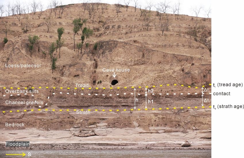
Fluvial
Fluvial terraces
terraces are morphostratigraphic
are morphostratigraphic units,
units, andand terrace
terrace deposits
deposits areare channel
channel sand
sand and/or
and/or gravel
faciesgravel
overlainfacies
by overlain by finefacies
fine overbank overbank facies
deposits deposits
bound bound strath
by bottom by bottom strath and
and upper upper
tread. tread.
Loess/paleosol
Loess/paleosol
deposits accumulatedeposits accumulate
on the tread in ouron the tread
studied areain(Figure
our studied area (Figure
9). Fluvial terraces9).are
Fluvial terraces are
geomorphologically
geomorphologically classified into strath terraces and fill terraces, and the only difference between
classified into strath terraces and fill terraces, and the only difference between them is that there is only
them is that there is only a thin layer of fluvial sands or gravels atop bedrock strath surfaces for strath
a thin layer of fluvial sands or gravels atop bedrock strath surfaces for strath terraces [80]. Practically,
terraces [80]. Practically, different thicknesses (h1 in Figure 9) of the “thin layer” have been used
different
whenthicknesses
a terrace is (h1 in Figure
assigned 9) of the
as a strath “thin
terrace in layer” have
the field. Thebeen used varies
thickness when from
a terrace
aboutisYou can also read