Effects of Frozen Soil on Soil Temperature, Spring Infiltration, and Runoff: Results from the PILPS 2(d) Experiment at Valdai, Russia
←
→
Page content transcription
If your browser does not render page correctly, please read the page content below
334                                    JOURNAL OF HYDROMETEOROLOGY                                                            VOLUME 4

   Effects of Frozen Soil on Soil Temperature, Spring Infiltration, and Runoff: Results
                    from the PILPS 2(d) Experiment at Valdai, Russia
   LIFENG LUO,a ALAN ROBOCK,a KONSTANTIN Y. VINNIKOV,b C. ADAM SCHLOSSER,c ANDREW G. SLATER,d
      AARON BOONE,e HARALD BRADEN,f PETER COX,g PATRICIA DE ROSNAY,h ROBERT E. DICKINSON,i
    YONGJIU DAI,j QINGYUN DUAN,k PIERRE ETCHEVERS,e ANN HENDERSON-SELLERS,l NICOLA GEDNEY,m,*
     YEVGENIY M. GUSEV,n FLORENCE HABETS,e JINWON KIM,o EVA KOWALCZYK,p KENNETH MITCHELL,q
    OLGA N. NASONOVA,n JOEL NOILHAN,e ANDREW J. PITMAN,r JOHN SCHAAKE,k ANDREY B. SHMAKIN,s
   TATIANA G. SMIRNOVA,t PETER WETZEL,u YONGKANG XUE,v ZONG-LIANG YANG,w AND QING-CUN ZENGj
                        a
                            Department of Environmental Sciences, Rutgers University, New Brunswick, New Jersey
                                     b
                                       Department of Meteorology, University of Maryland, College Park, Maryland
                             c
                              Goddard Earth Sciences and Technology Center, NASA GSFC, Greenbelt, Maryland
                                                      d
                                                        CIRES, University of Colorado, Boulder, Colorado
                                                             e
                                                              Météo-France/CNRM, Toulouse, France
                                  f
                                   Agrometeorologic Research, German Weather Service, Braunschweig, Germany
                        g
                          Hadley Centre for Climate Prediction and Research, Bracknell, Berkshire, United Kingdom
                                             h
                                               Laboratoire de Meteorologie Dynamique du CNRS, Paris, France
                      i
                       School of Earth and Atmospheric Sciences, Georgia Institute of Technology, Atlanta, Georgia
                                    j
                                     Institute of Atmospheric Physics, Chinese Academy of Sciences, Beijing, China
                                                     k
                                                      NOAA/Office of Hydrology, Silver Spring, Maryland
                                       l
                                        Australian Nuclear Science and Technology Organisation, Sydney, Australia
                                         m
                                           Meteorology Department, Reading University, Reading, United Kingdom
                                                          n
                                                           Institute of Water Problems, Moscow, Russia
                  o
                    Department of Atmospheric Sciences, University of California, Los Angeles, Los Angeles, California
                                               p
                                                Division of Atmospheric Research, CSIRO, Aspendale, Australia
                                         q
                                           NOAA/NCEP, Environmental Modeling Center, Camp Springs, Maryland
                                      r
                                       Department of Physical Geography, Macquarie University, Sydney, Australia
                                                             s
                                                               Institute of Geography, Moscow, Russia
                                                   t
                                                    NOAA/Forecast Systems Laboratory, Boulder, Colorado
                               u
                                 Mesoscale Dynamics and Precipitation Branch, NASA GSFC, Greenbelt, Maryland
                          v
                           Department of Geography, University of California, Los Angeles, Los Angeles, California
                                           w
                                            Department of Geological Sciences, University of Texas, Austin, Texas

                                   (Manuscript received 5 June 2002, in final form 4 October 2002)

                                                             ABSTRACT
               The Project for Intercomparison of Land-Surface Parameterization Schemes phase 2(d) experiment at
             Valdai, Russia, offers a unique opportunity to evaluate land surface schemes, especially snow and frozen
             soil parameterizations. Here, the ability of the 21 schemes that participated in the experiment to correctly
             simulate the thermal and hydrological properties of the soil on several different timescales was examined.
             Using observed vertical profiles of soil temperature and soil moisture, the impact of frozen soil schemes
             in the land surface models on the soil temperature and soil moisture simulations was evaluated.
               It was found that when soil-water freezing is explicitly included in a model, it improves the simulation
             of soil temperature and its variability at seasonal and interannual scales. Although change of thermal
             conductivity of the soil also affects soil temperature simulation, this effect is rather weak. The impact of
             frozen soil on soil moisture is inconclusive in this experiment due to the particular climate at Valdai, where
             the top 1 m of soil is very close to saturation during winter and the range for soil moisture changes at the
             time of snowmelt is very limited. The results also imply that inclusion of explicit snow processes in the
             models would contribute to substantially improved simulations. More sophisticated snow models based on
             snow physics tend to produce better snow simulations, especially of snow ablation. Hysteresis of snow-
             cover fraction as a function of snow depth is observed at the catchment but not in any of the models.

  * Current affiliation: Hadley Centre for Climate Prediction and Research, Bracknell, Berkshire, United Kingdom.

  Corresponding author address: Alan Robock, Department of Environmental Sciences, Rutgers University, 14 College Farm Road, New
Brunswick, NJ 08901-8551.
E-mail: robock@envsci.rutgers.edu

q 2003 American Meteorological Society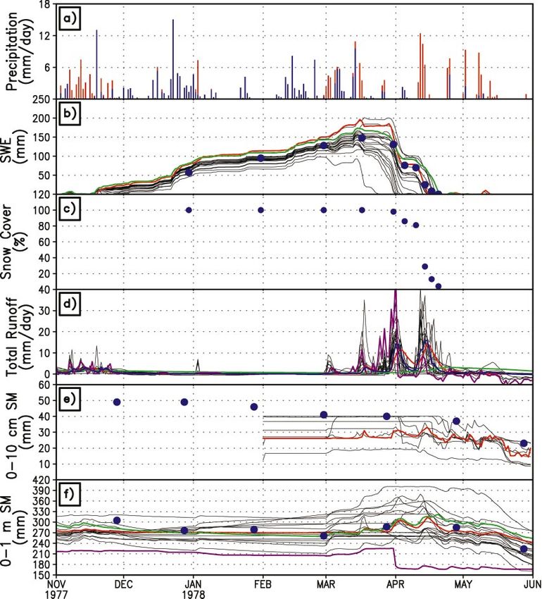
APRIL 2003                                         LUO ET AL.                                                                 335

1. Introduction                                                TABLE 1. Participating land surface schemes. Schlosser et al. (2000)
                                                             gives references for all the PILPS 2(d) schemes. Soil temperature:
   The land surface is an important component of the         ZS 5 zero storage; FR 5 force–restore; HC 5 heat conduction.
climate and weather system. The numerical expression                                                           Soil     Frozen
of land surface processes plays an important role in both             Model              Contact(s)         temperature soil?
climate and weather forecast models (e.g., Henderson-         1    AMBETI           H. Braden                  HC           Yes
Sellers et al. 1993; Gedney et al. 2000). As part of the      2    BASE             A. Slater                  HC           Yes
lower boundary of the atmosphere, the land surface is                               C. Desborough
strongly connected with atmospheric variations in sev-                              A. Pitman
                                                              3    BATS             Z. L. Yang                 FR           No
eral ways. By affecting water and energy flows between                              R. E. Dickinson
the land surface and the atmosphere, the thermal and          4    BUCKET           C. A. Schlosser            ZS           No
hydrological status of the soil is strongly connected with    5    CLASS            D. Verseghy                HC           Yes
the atmosphere. A large number of land surface schemes        6    CROCUS           P. Etchevers               HC           No
                                                              7    CSIRO            E. Kowalczyk               HC           Yes
(LSSs) have been designed to simulate land surface pro-       8    IAP94            Y. Dai                     HC           Yes
cesses in a variety of numerical ways. Models include         9    ISBA             F. Habets                  FR           Yes
all the important processes but might emphasize dif-                                J. Noilhan
ferent ones depending on their specific goals.               10    MAPS             T. Smirnova                HC           No
   The Project for Intercomparison of Land-Surface Pa-       11    MOSES            P. Cox                     HC           Yes
                                                             12    NCEP             K. Mitchell                HC           Yes
rameterization Schemes (PILPS) aims to improve un-                                  Q. Duan
derstanding of the parameterization of interactions be-      13    PLACE            A. Boone, P. Wetzel        HC           No
tween the atmosphere and the continental surface in          14    SECHIBA2         P. de Rosnay               HC           No
climate and weather forecast models (Henderson-Sellers                              J. Polcher
                                                             15    SLAM             C. Desborough              HC           Yes
et al. 1993, 1995). PILPS phase 2(d) (Schlosser et al.       16    SPS              J. Kim                     HC           Yes
2000) was designed to investigate land surface simu-         17    SPONSOR          A. B. Shmakin              HC           Yes
lations in a climate with snow and seasonally frozen         18    SSiB             Y. Xue                     FR           No
soil, making use of a set of meteorological and hydro-                              C. A. Schlosser
logical data spanning 18 yr (1966–83) from a grassland       19    SWAP             Y. M. Gusev                FR/ZS        Yes
                                                                                    O. N. Nasonova
catchment at the Valdai water-balance research station       20    UGAMP            N. Gedney                  HC           No
in Russia (Vinnikov et al. 1996; Schlosser et al. 1997).     21    UKMO             P. Cox                     HC           No
This offline experiment uses meteorological and radi-
ation data as forcing and hydrological data to evaluate
the LSS performances. A pilot study (Schlosser et al.        lation and five additional simulations designed to ad-
1997) using two LSSs, a simple bucket hydrology model        dress the sensitivity of the LSSs to downward longwave
(Budyko 1956; Manabe 1969) and a more complex bio-           radiation forcing, and the timescale and causes of sim-
sphere model, the Simplified Simple Biosphere Model          ulated hydrological variability (Schlosser et al. 2000).
(SSiB; Xue et al. 1991), illustrated the suitability of      Schlosser et al. (2000) focused on the hydrological out-
these datasets for stand-alone simulations.                  puts of model simulations requested by PILPS 2(d) and
   There are several advantages in the PILPS 2(d) ex-        compared the models’ performances against observed
periment compared with other PILPS phase 2 experi-           data on seasonal and annual timescales. They concluded
ments. The seasonal snow cover at Valdai allows us to        that the models’ root-zone soil moisture falls within the
evaluate snow schemes in the participant LSSs, exam-         observed spatial variability in nearly all cases, which
ining both seasonal cycles and interannual variations.       indicates that models can capture the broad features of
Seasonally frozen soil also offers a unique opportunity      soil moisture variations. They analyzed the water-flux
to check the model simulations of soil temperature and       partition on an annual basis and found that nearly all
the frozen soil schemes, if present. (When the soil tem-     the models partition the incoming precipitation into
perature is below 08C, it is the water in the soil that is   evaporation and runoff in a manner similar to obser-
frozen. Therefore, whenever we use the term frozen soil      vations in a broad sense. But they also pointed out that
we really mean frozen soil water.) Since runoff simu-        there is quite a bit of intermodel variability of the ratio
lation is affected both by snow and the partitioning of      of evaporation to runoff partitioning. Since the major
meltwater in the models, the role of the frozen soil phys-   runoff event takes place in the spring when snow is
ics in the partitioning of meltwater can be evaluated        melting, the partition of the meltwater into infiltration
based on daily observations of runoff and soil temper-       or runoff at this time contributes considerably to the
atures. Additionally, the Valdai experiment ran for 18       annual water budget. They concluded that a detailed
yr, allowing both the seasonal cycle and interannual var-    study during the melt period was needed to further ad-
iations to be investigated.                                  dress the reasons for these variations.
   Twenty-one LSSs (Table 1) of varying complexity              Slater et al. (2001) conducted a further detailed anal-
and based on different modeling philosophies partici-        ysis of the snow schemes in these models and compared
pated in PILPS 2(d). They performed a control simu-          them with observations from Valdai available then, and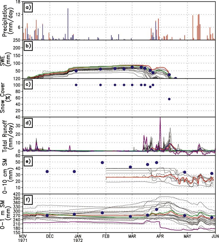
336                               JOURNAL OF HYDROMETEOROLOGY                                                        VOLUME 4

concluded that the models are able to capture the broad                  TABLE 2. Observational dataset at Valdai.
features of the snow regime on intra- and interannual        Meteorological data from meteorological station Priusadebny: taken
bases. They indicated that snow evaporation, snow al-        every 3 h, 1966–83
bedo, and snow-cover fraction have a large impact on           Precipitation
the snow simulations during ablation.                          2-m air temperature
   In spite of these previous analyses of the PILPS 2(d)       Pressure
                                                               Humidity
experiment, the role of frozen soil schemes in affecting       Wind speed
soil thermal properties, spring runoff, and infiltration
                                                             Hydrological data from Usadievskiy catchment
has not been studied before. Different snow-cover frac-
                                                               Total soil moisture in the top layer every 10 cm down to 1-m
tion formulations were discussed by Slater et al. (2001),        depth: 1 to 3 times per month, 1966–85
but no observations were available then to evaluate these      Discharge: daily, 1966–85
models. The objective of this study is to take advantage       Depth of groundwater table: monthly, 1960–90
of PILPS 2(d) results that have not been analyzed before       Water equivalent snow depth: irregularly, 1960–90
                                                               Soil surface evaporation: 10-day period sum from late spring to
and new datasets to examine these issues. Specifically,          early autumn, 1966–85
we will focus on answering the following questions: 1)         Snow cover fraction, snow thickness, and snow density: irregu-
How well do land surface models with and without fro-            larly, 1966–85
zen soil schemes simulate soil temperature, and what is        Freezing/melting depth: irregularly, 1966–85
the impact of the frozen soil scheme on soil temperature       Groundwater depth: every 5 days at different sites inside the
                                                                 catchment, 1966–85
simulations? 2) How well do land surface models sim-
ulate spring runoff and soil moisture, and what is the       Data from meteorological station (Priusadebny)
impact of the frozen soil scheme on the soil moisture          Soil surface temperature: daily, 1967, 1971–85
                                                               Soil temperature at 20, 40, and 80 cm: daily, 1967, 1971–85
and runoff simulations? 3) What is the role of the snow        Soil surface evaporation: 10-day period sum from late spring to
model in land surface modeling over cold regions?                early autumn, 1966–85
   In the next section we briefly summarize the obser-         Surface albedo: irregularly, 1966–85
vational data used in the experiment, and describe in
detail new data that we have recently acquired and used
for the first time. Section 3 gives the analysis, and dis-   downward shortwave radiation is strong during the 18-
cussion and conclusions are presented in section 4.          yr, with the absolute variability greater in the summer
                                                             than in winter. The amplitude of the interannual vari-
                                                             ation after removing the seasonal cycle can be up to 80
2. Description of the site and datasets
                                                             W m 22 on a monthly basis in the summer. The seasonal
   Descriptions of the continuous 18 yr (1966–83) of         variation of the downward longwave radiation is much
atmospheric forcing and hydrological data are given in       weaker than that of the downward shortwave radiation,
detail by Vinnikov et al. (1996) and Schlosser et al.        but the interannual variation of longwave radiation has
(1997). An overview of the dataset and a description of      a larger amplitude during the winter rather than summer.
additional observational data are given below.               This is because of the similar pattern for air temperature
   Table 2 lists the entire set of observations. We use      (Fig. 2). The monthly average air temperature gets down
most of them in this study. The data were obtained from      to 2108C in January. The temperature threshold to sep-
the Valdai water-balance station (58.08N, 33.28E) lo-        arate snow from rainfall was specified as 08C in this
cated in a boreal forest region (Fig. 1). Atmospheric        experiment (Schlosser et al. 2000), so most of the pre-
data were measured at the meteorological site Priusa-        cipitation was snow during the winter. The precipitation
debny, in the central part of the Valdai Experimental        shows some seasonality, varying from 1.5 to 3.5 mm
Station, including temperature, pressure, and humidity       day 21 on a monthly basis. The peak in October (Fig. 2)
measured at 2 m, and wind speed at 10 m. The atmo-           is quite important, as it is the major source of soil mois-
spheric data used as forcing by all the schemes were         ture recharge before the snow covers the ground. Al-
originally sampled at 3-h intervals and were interpolated    though precipitation has a small interannual variation
to 30-min intervals (or 5 min in some cases) using a         during the winter, the interannual variation of snow
cubic-spline interpolation procedure so that they could      depth is still rather large, as we will see in the next
be utilized by the models. Downward shortwave radi-          section. This can be attributed to the large interannual
ation and downward longwave radiation were simulated         variation in air temperature and longwave radiation dur-
based on observed cloudiness and temperature (Schlos-        ing the winter.
ser et al. 2000). The 21 LSSs were run for an 18-yr             Long-term hydrological measurements were taken at
period forced by these observations. The monthly av-         the Usadievskiy catchment at Valdai, which has an area
eraged downward shortwave radiation varies from about        of about 0.36 km 2 and is covered with a grassland mead-
20 W m 22 in the winter to 290 W m 22 in the short           ow (Fig. 1). The Usadievskiy catchment is a few ki-
summer each year (Fig. 2). The strong seasonal cycle         lometers away from the meteorology station at Priusa-
is mainly due to the large seasonal change of sun angle      debny. The hydrological data described by Vinnikov et
at this high latitude. The interannual variation of the      al. (1996) and Schlosser et al. (1997, 2000) contain only
APRIL 2003                                                   LUO ET AL.                                                                 337

  FIG. 1. Map of the Usadievskiy catchment at Valdai and its location, modified from Fig. 1 in Schlosser et al. (1997). Filled circles are
water-table measurement sites. Open circles with dashed lines indicated the snow measurement sites and routes, respectively. Discharge is
measured at the stream outflow point of the catchment (see bold bracket) at the lower left-hand corner of the catchment map. Filled triangles
indicate the measurement sites of soil freezing and thawing depths.

the monthly average evapotranspiration, runoff, liquid                  table is very shallow at this catchment and the variation
water equivalent snow depth [or, snow-water equivalent                  of the water table somewhat contributes to the discharge
(SWE)], top 1-m soil moisture, and water-table depth,                   measured at the outflow site. However, this modification
which are only enough to study general features of the                  is relatively small. As we cannot separate the total runoff
model performance on monthly and longer timescales.                     further into specific components, we compare this total
High-resolution observational data are needed to study                  runoff to the total runoff from the model simulations,
processes with short timescales. We recently obtained                   which is the sum of the surface runoff, drainage from
additional daily observational data from Valdai, includ-                the root zone, and the lateral flow.
ing daily soil temperature at different depths, soil mois-                 Soil moisture was measured using the gravimetric
ture at different depths every 10 days, surface albedo                  technique at 12 locations distributed over the Usadiev-
when snow is present, and daily catchment discharge.                    skiy catchment (Fig. 1), and the average of these 12
   The discharge from the catchment was measured daily                  measurements is used. The amount of water in each 10-
by a triangular weir and hydrometric flume at the catch-                cm soil layer down to 1 m was recorded at each mea-
ment outflow site at Usadievskiy (Fig. 1). If the water                 surement. The estimated error of this technique is about
head at the weir did not exceed 100 mm, the discharge                   61 cm for the top 1-m soil moisture (Robock et al.
was calculated following an empirical relationship be-                  1995). Soil moisture was usually sampled three times a
tween heads and discharges for the catchment. The total                 month, on the 8th, 18th, and 28th. Sometimes, especially
discharge was converted to runoff rate by taking into                   when the ground was frozen, it was measured monthly
account the area of the catchment. We further modified                  on the 28th. Although only the root-zone [top 1-m in
the runoff to account for the monthly variations in the                 this catchment, as specified by Schlosser et al. (2000)]
observed catchment-average water-table depth follow-                    soil moisture was requested in the control run from the
ing Schlosser et al. (1997). This is because the water                  schemes, the multidepth observations will help us un-
338                                   JOURNAL OF HYDROMETEOROLOGY                                                            VOLUME 4

              FIG. 2. Seasonal and interannual variation of the major atmospheric forcings on a monthly scale in the PILPS
                2(d) experiment. (left) The mean seasonal cycles and (right) the monthly and seasonal anomaly contours.

derstand the water flow inside the soil during the winter            The averaged number of measurement times each winter
and the melting period. Since the observations are only              was about 13. The snow begins accumulating in late
taken three times a month, and in some cases only once               November each year and melts around the next April.
a month, and soil moisture is a moisture reservoir and               The maximum snow depth and the time and duration
not a flux, the monthly averaged value is not really                 of melting varied from year to year (Fig. 3). Some other
suitable for model evaluation. Therefore, as in many                 snow characteristics were also observed at Valdai during
other studies, we use the soil moisture at the end of                winter. The snow depth was measured whenever SWE
each month (i.e., on the 28th) to study the seasonal and             was measured at the snow courses, and the snow density
interannual variations.                                              was derived from them. The snow-cover fraction was
   SWE was measured irregularly during the season at                 also recorded based on all the snow measurements.
44 locations inside the catchment (Fig. 1) when snow                 Since this is a relatively flat catchment covered with
was present and more frequently during snow ablation.                grass the snow-cover fraction is 1 most of the winter,
APRIL 2003 LUO ET AL. 339 FIG. 3. Observed time series of snow water equivalent (SWE, mm, filled circles) and the depths (mm) of the top and bottom of the frozen soil layer for each year. The gray dashed lines are observations from each individual location and the black lines are the average. but it can vary dramatically during spring snowmelt Therefore, it measured the snow surface temperature (Fig. 4). The surface albedo was measured at the me- when snow was present and soil surface temperature at teorological site Priusadebny approximately 4 km from other times. We use these data, keeping in mind that the Usadievskiy catchment. It was measured with a pyr- they might differ slightly from the situation at the Usa- anometer at about 1.5 m above the surface at local noon- dievskiy catchment. time. The pyranometer measured downward and upward Besides the soil temperature, the depths of the top shortwave radiation alternatively with the same sensor and bottom of the frozen soil layer were measured sev- facing up and down. The field of view of the sensor is eral times each winter at six locations inside the catch- relatively small when it faces downward due to its low ment (Fig. 1). A plastic pipe filled with water was placed mounting point. Therefore the representativeness of the vertically into the soil. It was extracted from the soil at surface albedo observation is unreliable for the catch- the time of observations to measure the position of the ment although the two sites are very close in distance frozen layer. Even if soil temperature is relatively ho- and surface characteristics. For this reason, the surface mogeneous over a small distance, the thickness of the albedo observations are not used in this study, but the frozen soil layers can have a much larger variation from data are introduced here. one point to another due to naturally heterogeneous soil The soil temperature was measured daily at the me- moisture fields. The spatial heterogeneity of soil mois- teorology site at Priusadebny. Thermometers were ture and frozen soil thickness, however, is beyond the placed vertically into the soil with the mercury bulbs at scope of this study. We use the averaged thickness from 20, 40, 80, and 120 cm below the surface and only five of those six observations to represent the catchment- extracted at the time of reading. The surface temperature averaged values while keeping in mind that this quantity was measured with a thermometer lying horizontally on has larger spatial variations (Fig. 3). One observation the surface with the bottom half of the mercury bulb was always very different from the other five, which covered by soil or snow. If the surface was covered by makes it less representative of the whole catchment al- snow, the thermometer was put on the snow surface. though the observation itself might be correct.
340                                   JOURNAL OF HYDROMETEOROLOGY                                                           VOLUME 4

                FIG. 4. The observed relationship between (a) snow depth and snow-cover fraction, and (b) SWE and
              snow-cover fraction. The numbered arrows indicate the possible path of changes of snow-cover fraction and
              SWE during a winter. See text for discussion. Observations are shown for the entire 18-yr period at Valdai.

   The maximum frozen soil thickness has a very large                accumulation at the soil surface. For all these reasons,
interannual variation (Fig. 3). The soil froze to a depth            correct soil temperature simulation is very important.
of more than 500 mm in the winter of 1971/72 but there
was virtually no frozen soil in the winter of 1974/75.
There was a general tendency for the soil to be frozen                  1) SOIL TEMPERATURE SCHEMES AND
more deeply when there was less snow and the tem-                           REPRESENTATION OF THERMAL EFFECT OF
perature was colder, as expected. The correlation be-                       FROZEN SOIL
tween the frozen depth and the snow depth is about 0.3,                 Different approaches are currently implemented in
positive but relatively small.                                       different land surface models to simulate soil temper-
                                                                     ature and ground heat fluxes (Table 1). They can be
3. Analysis                                                          simply grouped into the following three categories.
   In this section, we first study soil temperature sim-               (i) Zero-storage approach
ulations. We compare models with a frozen soil scheme
to those without, and to observations, to understand the               This approach can be generally expressed by the fol-
thermal effects of an explicit frozen soil scheme. Then              lowing equation:
the hydrological effects of the frozen soil scheme on
infiltration are analyzed by comparing the soil moisture                               R n 2 LE 2 H 2 G 5 0,                     (1)
change and runoff simulations during spring snowmelt                 where R n (W m 22 ) is net radiation, LE (W m 22 ) is latent
with the observations. The last part of this analysis fo-            heat, H (W m 22 ) is sensible heat, and G (W m 22 ) is
cuses on the hysteresis of snow-cover fraction and its               ground heat flux. A typical bucket model uses this ap-
impact on the snow simulation.                                       proach. It has only one soil layer in a hydrological sense
                                                                     and has no thermal layers, so the surface has no heat
a. Soil temperature and thermal effects of frozen soil               storage. The soil is assumed to be at a temperature that
                                                                     satisfies the energy balance at all times and there is no
   Soil temperature is an important factor in land surface           thermal capacity to the soil. Therefore there is no ex-
and atmospheric modeling. The soil surface temperature               plicit soil temperature simulation. The ground heat flux
directly affects longwave radiation, sensible heat flux,             is therefore ignored or prescribed in the energy budget.
and ground heat flux. A small error in soil temperature              The usage of this approach is justified by the fact that
at the surface can introduce a large error in upward                 the diurnal cycle of atmospheric forcing is removed.
longwave radiation. The wrong soil temperature profile
will produce the wrong ground heat flux, which in turn                 (ii) Force–restore approach
changes the energy budget at the surface and changes
other energy terms, such as sensible and latent heat                    This approach assumes periodic heating and uniform
fluxes. Additionally, soil temperature denotes the ex-               thermal properties of the soil; therefore, it requires con-
istence of frozen soil. It also affects the initial snow             siderable modification and tuning over inhomogeneous
APRIL 2003 LUO ET AL. 341
soil (Dickinson 1988). Soil temperature changes are de- also taken daily, we cannot evaluate the diurnal variation
scribed by of soil temperature in this study.
]Ts 1 2p
5 (R n 2 H 2 LE) 2 (T 2 Tm )
]t CT t1 s 2) SIMULATION OF SEASONAL SOIL TEMPERATURE
VARIATIONS
]Tm 1 2p
5 (Ts 2 Tm ) 2 (T 2 Tc ), (2) In PILPS 2(d), models provided average soil tem-
]t t1 t2 m
perature for two overlapping layers, the upper layer (0–
where t (s) is time, T s (K) is the surface temperature, 10 cm) and the lower layer (0–100 cm). The observa-
T m (K) is the daily mean surface temperature, T c (K) is tions are at the surface and four individual depths. To
the climatological deep temperature, C T (J K21 m 22 ) is avoid errors introduced by interpolation, we use the ob-
the surface soil/vegetation heat capacity per unit area, served surface temperature and 20-cm soil temperature
and t1 (s) and t 2 (s) are time constants. In this particular to compare with the models’ upper-layer soil temper-
form from the interactions between the soil, biosphere, atures, and the observed 40- and 80-cm soil tempera-
and atmosphere scheme (ISBA; Mahfouf et al. 1995), tures to compare with the models’ lower layer. The sur-
T s is restored toward the mean surface temperature T m face temperature is really the snow surface temperature
with a time constant t1 of 1 day, and T m is restored when snow is present during winter. For convenience,
toward the climatological deep temperature T c updated we also group the 21 models into two groups and plot
with a time constant t 2 of 20 days. The temperature T c them against observations separately in different panels.
is updated monthly. Using this approach, the model may The monthly averaged surface temperature can be
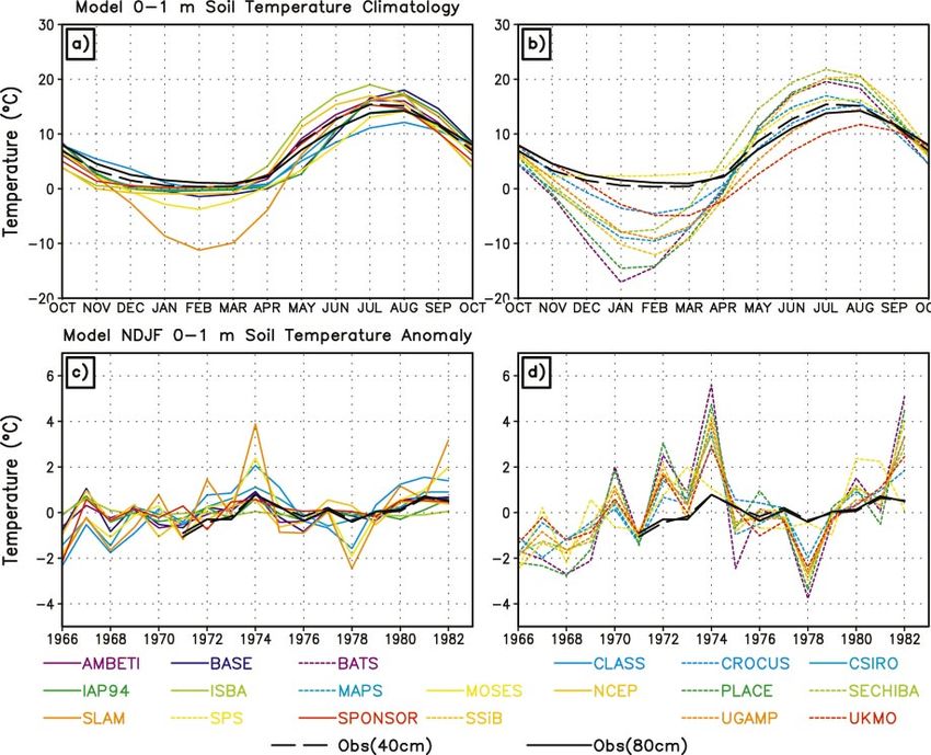
have one or more layers. Since the soil temperature is lower than 2108C during winter (Fig. 5) while the 20-
restored toward climatology while allowing some de- cm soil temperature is very close to 08C at the same
gree of variation, if the climatological values are ac- time. The 40- and 80-cm soil temperatures are normally
curate, modeled soil temperature will not drift. above 08C on a monthly basis (Fig. 6). Therefore, the
largest temperature gradient exists between the surface
(iii) Heat conduction approach temperature and the 20-cm level.
No matter which approach is used to simulate soil
This approach explicitly solves the heat conduction temperature in the models, the phase of the seasonal
equation to get the soil temperatures for different model
cycle of soil temperature is well captured for the upper
layers,
layer, given the correct atmospheric forcing, especially
air temperature (Figs. 5a,b). The lower-layer simulation,
Cs
]Tg
]t
5
[ ]
] ]Tg
g
]z ]z
however, shows phase differences of up to about 1
month among models and between models and obser-
vations (Figs. 6a,b).
G5g
]Tg
]z) z50
5 R n 2 LE 2 H The soil temperature shows a large scatter among
models in both layers, especially during winter. Due to
the framework of this comparison, we would expect the
G5g
]Tg
]z) z52h
50 or Tg | z50 5 Ts , (3)
models’ upper-layer soil temperature to be bounded by
the two observations at the surface and 20 cm, and the
lower-layer soil temperature to be bounded by the ob-
where T g (K) is the soil temperature at a particular layer, servations at 40 and 80 cm. The upper layer shows
g (J K21 m 21 ) is the soil thermal conductivity, and C s reasonably good agreement between models in group A
(J K21 m 22 ) is the volumetric heat capacity of the soil. and observations from April to November. Two models
This approach might also have a layer with heat storage in group B overestimate the upper-layer soil temperature
at the surface and not just an instantaneous energy bal- during this period while others are reasonably good.
ance. To solve the equation, the model needs to have During winter, models in group A have the upper-layer
several layers and to have them discretized in a proper soil temperature close to observations at 20 cm except
way. Thermal capacities and thermal conductivity of all the ISBA, Met Office Surface Exchange Scheme (MO-
layers are needed to perform the calculation. This ap- SES), and Simple Land–Atmosphere Mosaic (SLAM)
proach is considered to be the most realistic one. Many models, while models in group B have a much colder
land surface models take this approach, such as the Pa- upper-layer soil temperature, with the exception of SSiB
rameterization for Land–Atmosphere–Cloud Exchange (Figs. 5a,b). The lower-layer soil temperature shows
(PLACE; Wetzel and Boone 1995) and Mesoscale Anal- even larger differences between group A and group B
ysis and Prediction System (MAPS; Smirnova et al. (Figs. 6a,b). The observed soil temperatures at 40 and
1997) (Table 2). 80 cm are very close to 08C during winter. Almost all
Because the requested output from models in this models in groups A (Fig. 6a) produce very similar soil
experiment is at the daily scale and the observations are temperature simulations, but most of the models in342 JOURNAL OF HYDROMETEOROLOGY VOLUME 4
FIG. 5. (top) The mean seasonal cycle of the 0–10-cm soil temperature from all models compared with observations at (a) the surface
and (b) 20 cm. (bottom) Interannual anomalies of the 0–10-cm soil temperature averaged for the Nov–Feb period from all models compared
with observations. (a), (c) Models with frozen soil schemes are plotted in solid lines, while (b), (d) models without are plotted with dashed
lines.
group B (Fig. 6b) produce much colder soil columns would be best supported if we could rerun the simu-
during winter and much warmer during summertime. lations with the models that have a frozen soil scheme
The aforementioned differences can be attributed to but with the scheme disabled. Since this study is a con-
the existence of the frozen soil schemes. As indicated tinuation of postexperiment analysis based upon the
in Table 1 and in Figs. 5 and 6 (group A are models availability of a new observational dataset, and since
with a frozen water scheme and are plotted in solid lines models are continuously being improved, rerunning the
in panels a and c, group B are models without a frozen same version of those models is not possible at this
water scheme and are plotted in dashed lines in panels stage. However, these simple comparisons are already
b and d), models with an explicit frozen soil scheme good evidence of the impact of a frozen soil scheme on
give a much more realistic soil temperature simulation soil temperature simulations.
during winter than those without a frozen soil scheme.
Energy is released when the soil starts to freeze due to
3) SIMULATION OF INTERANNUAL VARIATION OF
the phase change of water. The energy is then used to
SOIL TEMPERATURE
warm up the soil and to keep it from extreme cold. This
simple mechanism works in the real world and in the The observed surface temperature shows strong in-
models. So once a frozen soil scheme is included in a terannual variations while the other levels have a much
land surface model, the soil temperature will not get weaker interannual variation during winter (Figs. 5 and
extremely cold at the lower and deep layers. This result 6). As mentioned above, the observations show a gen-APRIL 2003 LUO ET AL. 343
FIG. 6. Same as in Fig. 5, but for the top 0–100-cm soil temperature from models. The observations are at depths of 40 and 80 cm.
eral tendency for the soil to get very cold when snow temperature variations from the surface down to the
is thinner during winter. Nearly all models are able to deep soil on all timescales.
capture this variability to some extent. Models with a Besides this direct effect, frozen soil schemes have
frozen soil scheme have a much smaller amplitude of another effect on soil temperature and ground heat flux
interannual variation for both layers (Figs. 5c and 6c). simulations. The change of thermal conductivity of a
They are also much closer to the amplitude of the ob- soil column when soil water turns to ice is soil moisture-
served variations. Models without a frozen soil scheme dependent. Generally speaking, as in the case of rather
have a 3–5 times larger amplitude of variation compared wet soil at Valdai during winter, frozen soil has a larger
to observations for the lower layer (Figs. 5d and 6d). thermal conductivity than the unfrozen soil with the
same water content due to the larger thermal conduc-
tivity of ice as compared to liquid water. The high ther-
4) ROLE OF FROZEN SOIL SCHEMES IN SOIL
mal conductivity makes the heat transport inside the soil
TEMPERATURE SIMULATION
more efficient. Due to the downward temperature gra-
A physically based frozen soil scheme releases energy dient (colder at the surface and warmer in the deep soil),
as the soil water changes phase from liquid to solid. the upward ground heat flux becomes larger when soil
The energy slows the cooling of the soil to keep the freezes. If this effect is also parameterized in the frozen
surface temperature from becoming extremely cold at soil scheme, it tends to cool the soil column, which
the beginning of the winter. The process of soil freezing makes the soil temperature lower (Smirnova et al. 2000).
effectively increases the thermal inertia of the soil at But this effect is probably weaker than the direct effect
the beginning of winter, which efficiently damps large discussed above due to water phase changes.344 JOURNAL OF HYDROMETEOROLOGY VOLUME 4
Models with frozen soil all include the changes in considerable scatter among the models and there were
heat capacity and thermal conductivity, but in slightly differences between the models and the observations.
different ways. Soil Water-Atmosphere–Plants land sur- Here, we will not study the soil moisture simulation
face parameterization science (SWAP) does this simply during the whole period but rather focus on the winter
by changing the values by a certain factor when the soil and spring when frozen soil exists. Major runoff events
is frozen. A more explicit method is to calculate the happen during the spring snowmelt at Valdai, and we
actual ice and water content in the soil to determine the focus on this period for runoff, even though there is the
heat capacity and thermal conductivity [e.g., Australia’s second peak during the fall. Because of the large in-
Commonwealth Scientific and Industrial Research Or- terannual variation of snow during winter and the snow
ganisation (CSIRO)]. Another important difference is ablation period in the spring, and the temporal scale of
how much liquid water models allow to exist when soil the runoff processes, mean values of snow and runoff
temperature is below 08C. Some schemes do not allow calculated based on the 18 yr are not good candidates
liquid water to exist below 08C, while others have liquid to use in the study. Instead, we use several individual
water inside the frozen soil layer (e.g., MOSES; Cox et years as examples. Based on observations, the following
al. 1999). This difference eventually affects the soil tem- three springs are chosen: 1972, 1976, and 1978. The
perature simulation, as well as hydraulic properties of winter of 1971/72 had the least snow and the winter of
the soil, as discussed later. 1975/76 had the most snow during the 18 yr. The winter
of 1977/78 had a snow depth close to the average over
5) MODEL STRUCTURE AND SOIL TEMPERATURE the 18 yr. Looking at these 3 yr gives us a more com-
SIMULATION prehensive picture of the models’ performances.
As shown in Fig. 2 in Schlosser et al. (2000), the 21
participants have a wide range of the number of soil 1) RUNOFF SIMULATION DURING SNOWMELT
thermal layers, from the simplest 0 layers in the bucket
model to 14 layers (Anwendung des Evapotranspira- As a consequence of the spring snowmelt, a large
tions-modells; AMBETI; Braden 1995). A heat con- amount of water becomes available for infiltration and
duction approach needs at least two layers to solve the runoff. In the real world, if the infiltration capacity or
heat conduction equation. Ideally, the more layers and the maximum infiltration rate is not large enough to let
the thinner the layers get, the more chance there is to all the available water go into the soil, surface runoff
accurately simulate the soil temperature profile. How- will be generated. The infiltration capacity is controlled
ever, practical accuracy is often limited by the absence by the soil texture and soil moisture conditions. Whether
of information on vertical profiles of parameters or even the soil is frozen or not is another key factor that in-
the vertical mean parameters. A thinner layer also re- fluences the infiltration capacity.
quires a shorter time step. The balance between practical Largely influenced by the snow simulation, most
accuracy and efficiency is another factor that limits mod- models produce a slightly earlier runoff than observed
el performance. AMBETI has the best soil temperature (Figs. 7–9). Generally, the earlier the snow ablation
simulation among all the models (not shown here). takes place in the model, the earlier the runoff will be;
ISBA (Mahfouf et al. 1995; Noilhan and Mahfouf 1996) the faster the snow melts, the higher the runoff peak;
has only two thermal layers with the second one going and the greater the snow amount, the more total volume
from 10 cm to 2 m. The second-layer soil temperature of water available for runoff and infiltration. Sublima-
is fixed at 08C when the top layer is frozen. This con- tion also affects the partition of snow water. Slater et
figuration produces large upward heat fluxes due to the al. (2001) looked at the scatter in accumulated subli-
large temperature gradient and thickness of the second mation as simulated by models and found that net snow
layer. As discussed by Slater et al. (2001), the model sublimation varies considerably among the models. This
structure, especially the way that the snow layer and also affects the amount of snow available for runoff and
top soil layer are connected, also affects the soil tem- infiltration when it melts. In this sense, the snow sim-
perature simulation. An implicit scheme lumps snow ulation has a large impact on the performance of the
and surface soil and vegetation together, so the soil tem- runoff simulation. In Figs. 7–9 we highlight the snow
perature tends to be colder. This is different from models metamorphism model CROCUS in red in several panels.
that diffuse energy between a separate snow layer and CROCUS gives a good simulation of snow in almost
the top soil layer. all years, especially of the timing of snowmelt. This in
turn provides the correct amount of water to infiltration
and runoff at the right time. The result is an almost
b. Runoff and soil moisture simulation in spring and
perfect match to the runoff curves (Figs. 7d–9d). This
the hydrological effect of a frozen soil scheme
is especially important given the simplicity of the mod-
As shown by Schlosser et al. (2000), nearly all models el’s runoff scheme, where runoff rate is only determined
simulated the correct seasonal cycle of root-zone soil by soil moisture with a linear relationship.
moisture fairly well, while at the same time there was In addition to snow, the infiltration (or partition)APRIL 2003 LUO ET AL. 345 FIG. 7. Time series of the major hydrological variables simulated by models for the winter of 1971/72. (a) Precipitation (mm day 21 ); Blue indicates snowfall and red indicates rain. (b) Snow water equivalent (SWE, mm). Blue dots indicate observations. Models are plotted as black lines except CROCUS and SPS, which are highlighted in red and green, respectively. (c) Snow-cover fraction (%). Only observations are available. (d) Daily runoff (mm day 21 ). Blue curve is the observations. Models are plotted as black curves except CROCUS, SPS, and SPONSOR, which are highlighted in red, green, and purple, respectively. (e) Top 10-cm soil moisture (SM, mm). Blue dots are observations. Models are plotted as black curves except CROCUS, which is highlighted in red. SPS and SPONSOR do not have output for this layer. Model simulations of 0–10-cm soil moisture are only available from Feb to May in 1971–79. (f ) As in (e) but for top 1 m. Models are plotted as black curves except CROCUS, SPS, and SPONSOR, which are highlighted in red, green, and purple, respectively. scheme also affects the runoff. For example, the Snow– surface runoff. The runoff peaks more than 20 days later Plant–Snow model (SPS; Kim and Ek 1995) has a sat- than observed. The gradual release of water from the isfactory simulation of snow, but the runoff is totally soil also reduces the maximum rate of runoff tremen- wrong (Figs. 7d–9d, green curves). This is simply be- dously. The observed runoff rate can be as high as 15 cause the model partitions all the meltwater into infil- mm day 21 , while SPS has a maximum runoff rate of 2– tration and drainage takes place much more slowly than 3 mm day 21 .
346 JOURNAL OF HYDROMETEOROLOGY VOLUME 4
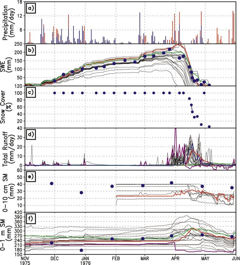
FIG. 8. Same as in Fig. 7 but for the winter of 1975/76.
2) SOIL MOISTURE SIMULATION ulation (Figs. 7g–9g, purple curves). A sudden soil
For the top 1 m of soil (Figs. 7f–9f), all nonbucket- moisture drop right after snowmelt might be caused by
type models can capture the soil moisture recharge after the extremely high hydraulic conductivity used in sev-
the snowmelt. Because at Valdai the top 1-m soil mois- eral time steps when soil becomes saturated with the
ture is close to field capacity [specified as 271 mm in melting water during the model integration. This soil
the PILPS 2(d) instructions] during most winters, the moisture drop also produces a spike in total runoff sim-
bucket is full and has no ability to accept any more ulation (Figs. 7d–9d). This makes it not follow the sea-
water. For Richard’s equation–based schemes, field ca- sonal cycle at all.
pacity is not explicitly used and neither is the maximum Observations show a soil moisture increase during
of soil-water content. One model (SPONSOR) seems to snowmelt in most years, even though the top 1 m of
have a numerical instability problem during this sim- soil is already close to or above field capacity. Then theAPRIL 2003 LUO ET AL. 347
FIG. 9. Same as in Fig. 7 but for the winter of 1977/78.
soil moisture gradually decreases after the snow dis- higher than field capacity and very close to saturation.
appears. This means that there is infiltration taking place The total soil-water content (including water and ice)
during snowmelt regardless of the soil moisture state decreases with depth almost linearly in the top 50 cm
before the melting or of the soil temperature. The water (not shown). This inverse soil moisture gradient was
table temporarily enters the top 1 m of soil, making the observed almost every September to the next April. This
soil moisture greater than the field capacity. This be- indicates that the surface soil layer might have a dif-
havior for this part of Russia was previously pointed ferent porosity from the rest of the soil column, while
out by Robock et al. (1998) in their Fig. 6. the experiment uses the same porosity for all levels. The
For the top 10-cm soil (Figs. 7e–9e), nearly all models underestimation in the model simulation is due to the
underestimate the soil moisture. As shown in obser- predefined soil porosity of 0.401 in the experiment, and
vations, the soil moisture in the top 10 cm is much therefore models cannot go above this.348 JOURNAL OF HYDROMETEOROLOGY VOLUME 4
3) ROLE OF A FROZEN SOIL SCHEME IN THE water and then let drainage and evaporation take place.
RUNOFF AND SOIL MOISTURE SIMULATION But this speculation is based on two assumptions: 1) the
soil is not saturated before the snowmelt so that infil-
In addition to the thermal effect of a frozen soil layer, tration can take place later on; 2) the soil is still totally
discussed earlier, another potential effect is that when frozen when snow is melting and there is no infiltration.
the soil is frozen or partially frozen, infiltration from In the PILPS 2(d) experiment, however, we do not see
the surface could be changed due to the change of soil a big difference in soil moisture simulations from mod-
structure, pore-size distribution of the soil, and the hy- els with or without frozen soil physics. As mentioned
draulic conductivity (Hillel 1998). The influence of above, the top 1 m of soil always reaches field capacity,
freezing on soil structure varies depending on many and the top 10 or 20 cm can be saturated during winter
factors, such as structural condition before freezing, soil in Valdai (Figs. 7–9). The water table rises into the root
type, water content, number of freeze/thaw cycles, freez- zone at this time. No matter whether a frozen soil layer
ing temperature, and freezing rate. In soil with a poor is included in a model or not, the change of soil moisture
structure, freezing can lead to a higher level of aggre- from before snow cover (normally November) to after
gation as a result of dehydration and the pressure of ice the snowmelt is very limited by the available pore space.
crystals. On the other hand, if the soil structure is well Nevertheless, the first assumption is valid in this case.
developed, expansion of the freezing water within the As shown in Fig. 3, however, the soil ice is melting
larger aggregates and clods may cause them to break when the snow is melting. The top of the frozen soil
down. This breakdown is enhanced when freezing oc- layer moves downward to a lower level, which leaves
curs so fast that the water freezes in situ within the the top part of the soil available for some infiltration.
aggregates, whereas during slow freezing the water can The winter of 1971/72 is the winter with the least snow
migrate from the aggregates to the ice crystals in the and thickest frozen soil. But when the snow melts, the
macropores. Freezing influences the permeability of frozen soil disappears from the top very quickly (Fig.
soils owing to the fact that ice impedes the infiltration 3). As we mentioned above, the heterogeneity of soil
rate. In partially frozen soil it is very likely that the freezing also allows surface water to find ways to in-
infiltration rate will be suppressed as a result of imped- filtrate somewhere else in the catchment. The second
ing ice lenses as well as structural changes. Current land assumption is invalid. Therefore, the influence of the
surface models do not simulate all these details but rath- frozen soil on infiltration is weak in the observations at
er try to model a simplified process. An ‘‘explicit’’ fro- Valdai. The difference in soil moisture simulations pro-
zen soil scheme will reduce the infiltration based on soil duced by frozen soil schemes between two groups of
temperature, soil ice content, and soil properties. An models (models with frozen soil and those without) can-
‘‘implicit’’ frozen soil scheme might totally stop water not be clearly distinguished from the differences caused
flow inside the soil (Mitchell and Warrilow 1987) by by any other sources of difference between models.
specifying that if the snow melts while the soil is still
frozen, the meltwater cannot infiltrate to recharge the
soil moisture and it will have to run off. Models that c. Snow-cover fraction simulation and role of snow
are parameterized for general circulation model uses schemes in land surface modeling
might not alter the infiltration capacity even when the The snow simulation in an LSS plays a very important
soil is frozen. They are designed to represent a large role in the energy and water budget. The snow albedo
region (one grid box in a low-resolution model) where changes the absorbed energy in the visible and near-
Hortonian surface runoff from frozen soil surface would infrared bands dramatically at the surface. As discussed
find its way into the soil elsewhere in the same grid above, the total snow amount will determine the amount
box, owing to heterogeneities in frozen soil and soil of available water for infiltration and runoff in spring.
freezing hydraulic conductivity (Cox et al. 1999). This Slater et al. (2001) studied the snow simulations in this
will also help us to understand the difference in the experiment and used the differences in snow evapora-
runoff simulations shown between CROCUS and SPS. tion, snow albedo, snow-cover fraction, and snow model
The latter is designed and calibrated to simulate pro- structure to explain the differences among the models.
cesses at a much larger spatial scale. This is why the As an extension of their study, this paper will also ad-
runoff is delayed for about 20 days compared with ob- dress the snow-cover fraction issue based on observa-
servations. On the contrary, the simple runoff param- tions.
eterization in CROCUS matches well the scale of this Surface albedo during winter depends on snow al-
catchment so that it can produce good simulations. We bedo, snow-cover fraction and underlying vegetation.
might speculate that the performance of these models Snow albedo depends on the physical state of the snow,
would be different or even reversed when applied at the especially snow grain-size, snow type, and contamina-
large scale for which SPS was developed. tion. But these quantities are always hard to measure
Presumably, an LSS with a frozen soil scheme will and quantify. Careful observations of snow albedo at
have less water in the soil after the snow is gone, while small scales (e.g., Warren and Wiscombe 1980; Warren
those without frozen soil will fill the soil column with 1982) have provided the basis for snow albedo simu-APRIL 2003 LUO ET AL. 349
lation in numerical models. To explicitly simulate these fall might be little. This effect is very well illustrated
processes by solving a full set of equations is compu- in 1976 (Figs. 8b,c). As a result of the late-season snow-
tationally expensive, so most land surface models take fall and subsequent increase of snow-cover fraction, we
a shortcut, using empirical relationships between snow expect the surface albedo to jump right up after the
albedo and other variables, such as temperature, age of snowfall. Then the snow-cover fraction decreases lin-
snow, and SWE. Different snow models may only con- early with SWE again until all the snow is gone. It is
sider a subset of these in the snow albedo formulation. easy to fit the data to get an empirical function at this
The snow-cover fraction is formulated as a linear or stage, but this linear relation is probably not universal
asymptotic function based on snow depth and surface and depends somewhat on the surface topography and
characteristics such as vegetation roughness. Of course, vegetation. Since none of the snow-cover fraction for-
the simplest model is to assume 100% coverage of snow mulas in the current models include this feature, the
when snow is present. Detailed information about al- lack of this effect can significantly affect the snow sim-
bedo and fractional cover formulas in the 21 LSSs in ulations.
PILPS 2(d) is listed in Table 2 of Slater et al. (2001).
SWE and snow-cover fractions were observed at 44
4. Discussion and conclusions
points inside the catchment so they more or less rep-
resent the whole catchment. The observed snow-cover The 18-yr offline simulations and observations from
fraction was 100% from the first observation during Valdai with inter- and intraannual variation of soil tem-
winter to the beginning of snowmelt (Figs. 7d–9d). Even perature, frozen soil depth, soil moisture, snow, and
with thin snow on the ground after the initial snowfall, runoff are a valuable resource for land surface model
the snow-cover fraction was high and the surface albedo validation and evaluation. It must be remembered, how-
was high. When models cannot correctly simulate snow- ever, that the model simulations used in this analysis
cover fraction, the surface albedo will be wrong even were conducted several years ago. Some of the models
with a correct snow albedo scheme. During snowmelt, have been improved since then, including improvements
with a fair amount of snow on the ground, the surface in response to the results of this PILPS 2(d) experiment,
albedo can be very low because the snow-cover fraction and, therefore, the results may not reflect the current
is low and because of a low snow albedo when melting. model performance. Most of these models also partic-
Because fresh snow has a much higher albedo than ipated in the PILPS 2(e) experiment and their current
old snow, snow albedo exhibits hysteresis in the rela- performance in cold region simulations is described by
tionship between total snow depth and snow albedo even Bowling et al. (2002a,b) and Nijssen et al. (2002). In
though it is the surface layer of snow that determines PILPS 2(e) most models include an explicit represen-
snow albedo. This hysteresis can be represented in mod- tation of frozen soil, no doubt partly in response to the
els that explicitly simulate the snow albedo based on results of PILPS 2(d). We hope, however, that the new
the top snow layer. Interestingly, the snow-cover frac- analyses presented here will lead to further improvement
tion at the Valdai grassland also exhibits hysteresis. For of model performances.
the same amount of snow, snow-cover fraction during Over a region like Valdai with seasonal snow cover
snow accumulation is always higher than during the and frozen soil, snow simulation is the most important
snowmelt period, especially for thin snow. As shown in feature for a land surface model to be able to simulate
Fig. 4b, there is a general linear relationship between components of the land surface hydrology correctly in
SWE and snow-cover fraction when snow covers less the spring. Snow affects the availability of water for
than 100% of the area. This linear relationship is from runoff and infiltration, affects the energy available for
observations during snowmelt and we can speculate that evapotranspiration through its albedo and indirect effect
the relationship between those two during snow accu- on resulting soil moisture, and affects soil temperature
mulation will have a smaller slope. by its blanketing effects. These effects are clearly dem-
To illustrate this snow-cover fraction hysteresis, the onstrated in the analyses of the PILPS 2(d) experiment
numbered arrows in Fig. 4b indicate the possible path here.
of changes of snow-cover fraction and SWE during a Based on observations, snow metamorphism has been
winter. Arrow 1 is the first snowfall at the beginning of introduced into some snow modules. Physical processes
the winter or late fall. This is a dramatic change in such as absorption of solar radiation with depth, phase
surface albedo and snow-cover fraction without heavy changes between solid and liquid water, and water trans-
snowfall. Arrow 2 is during the snow accumulation pe- mission through the snowpack have been added (e.g.,
riod, which lasts about 4 months. Arrow 3 is during the CROCUS; Brun et al. 1992). Brun et al. showed that
first several days of the melting when SWE decreases introduction of metamorphism laws into the snow model
quickly while the snow still covers the whole area. After significantly improved model performance. We also
that, snow-cover fraction decreases almost linearly with showed that more sophisticated snow schemes in land
SWE as indicated by arrow 4. If there is another snow- surface models, after careful calibration have the po-
fall during the melting period, it brings the snow-cover tential to produce a large improvement in hydrological
fraction back to 1.0 very quickly even though this snow- event simulations in a region where snow cover lasts350 JOURNAL OF HYDROMETEOROLOGY VOLUME 4
several months and water equivalent snow depth reaches Acknowledgments. We thank Nina Speranskaya for
several centimeters. Simple snow models can simulate the new Valdai data. We thank three anonymous re-
snow accumulation when the right critical temperature viewers for valuable recommendations. Figures were
for snowfall is chosen, but once snow starts to melt, drawn with GrADS, created by Brian Doty. This work
they do not have the ability to represent the real world, is supported by NOAA Grants NA56GPO212,
resulting in errors in the simulation of snow melting in NA96GPO392, and GC99-443b, and the New Jersey
terms of timing and total amount. Although there are Agricultural Experiment Station.
tunable parameters in simple snow models in most cas-
es, and there is always the possibility that the model
can be tuned to fit observations, the parameter values REFERENCES
would have to be case- and region-dependent, and even
then the model would not capture the real physics. A Bowling, L. C., and Coauthors, 2002a: Simulation of high latitude
hydrological processes in the Torne-Kalix basin: PILPS Phase
realistic parameterization of snow-cover fraction that 2(e). 1: Experiment description and summary intercomparisons.
relates the surface characteristics and represents the hys- Global Planet. Change, in press.
teresis is needed to improve the snow and surface energy ——, and Coauthors, 2002b: Simulation of high latitude hydrological
simulation. We have observed this important feature in processes in the Torne-Kalix basin: PILPS Phase 2(e). 3: Equiv-
alent model representation and sensitivity experiments. Global
the grassland catchment, but none of the models param-
Planet. Change, in press.
eterizes it into the snow model. This can potentially Braden, H., 1995: The model AMBETI: A detailed description of a
produce substantial errors in surface albedo simulation soil–plant–atmosphere model. Beitr. Dtsch. Wetterdienstes, 195,
and energy budget. 117 pp.
Frozen soil in the winter was expected to have a great Brun, E., P. David, and M. Sudul, 1992: A numerical model to sim-
ulate snow-cover stratigraphy for operational avalanche fore-
influence on the runoff and soil moisture simulation casting. J. Glaciol., 38, 13–22.
(Mitchell and Warrilow 1987; Pitman et al. 1999). But Budyko, M. I., 1956: Heat Balance of the Earth’s Surface (in Rus-
Pitman et al. (1999) were not able to show improvement sian). Gidrometeoizdat, 255 pp.
of runoff simulation when including soil ice in a Global Cherkauer, K. A., and D. P. Lettenmaier, 1999: Hydrologic effects of
Soil Wetness Project–type simulation. Cherkauer and frozen soils in the upper Mississippi River basin. J. Geophys.
Res., 104, 19 599–19 610.
Lettenmaier (1999) also found that including frozen soil Cox, P. M., R. A. Batts, C. B. Bunton, R. L. H. Essery, P. R. Rowntree,
in their LSS had a relatively small effect on soil moisture and J. Smith, 1999: The impact of new land surface physics on
and runoff. Even though snow is present, infiltration can the GCM simulation of climate and climate sensitivity. Climate
occur as the soil is not frozen near the top as meltwater Dyn., 15, 183–203.
percolates. Over a large region, Hortonian surface runoff Dai, Y.-J., and Q.-C. Zeng, 1997: A land-surface model (IAP94) for
climate studies. Part I: Formulation and validation in off-line
can always find its way to infiltrate somewhere in the experiments. Adv. Atmos. Sci., 14, 433–460.
domain owing to the fact that soil is not freezing ho- de Rosnay, P., J. Polcher, M. Bruen, and K. Laval, 2002: Impact of
mogeneously because of variation in soil texture, soil a physically based soil water flow and soil–plant interaction
structure, soil moisture, and soil temperature, and many representation for modeling large-scale land surface processes.
other factors. So inclusion of a frozen soil scheme has J. Geophys. Res., 107 (D11), 4118, doi:10.1029/2001JD000634.
Desborough, C. E., and A. J. Pitman, 1998: The BASE land surface
little effect on the simulations of soil moisture. model. Global Planet. Change, 19, 3–18.
Soil-water freezing has been proved to be very im- Dickinson, R. E., 1988: The force–restore model for surface tem-
portant in soil temperature simulation, however. We ob- peratures and its generalizations. J. Climate, 1, 1086–1097.
served a large temperature gradient at the near-surface Gedney, N., P. M. Cox, H. Douville, J. Polcher, and P. J. Valdes,
2000: Characterizing GCM land surface schemes to understand
soil during winter. This is attributed to the frozen soil,
their responses to climate change. J. Climate, 13, 3066–3079.
which releases heat when water changes phases from Henderson-Sellers, A., Z.-L. Yang, and R. E. Dickinson, 1993: The
liquid to solid, keeping the soil from getting extremely Project for Intercomparison of Land Surface Parameterization
cold. This effect is also found in models with a frozen Schemes. Bull. Amer. Meteor. Soc., 74, 1335–1350.
soil scheme, in both seasonal and interannual timescales. ——, A. J. Pitman, P. K. Love, P. Irannejad, and T. H. Chen, 1995:
The Project for Intercomparison of Land-surface Parameteriza-
These models produce much more realistic soil tem- tion Schemes (PILPS): Phases 2 and 3. Bull. Amer. Meteor. Soc.,
perature variations than those without a frozen soil 76, 489–504.
scheme. It has been found that soil temperature is a Hillel, D., 1998: Environmental Soil Physics. Academic Press,
dominant factor in determining the rate of soil carbon 771 pp.
cycling in the boreal forest (Nakane et al. 1997), and Kim, J., and M. Ek, 1995: A simulation of the surface energy budget
and soil water content over the HAPEX-MOBILHY forest site.
the timing of snowmelt and soil thaw is a major factor J. Geophys. Res., 100, 20 845–20 854.
in determining annual carbon uptake in a boreal region Mahfouf, J.-F., A. O. Manzi, J. Noilhan, H. Giordani, and M. Déqué,
(Sellers et al. 1997). As land surface schemes begin to 1995: The land surface scheme ISBA within the Météo-France
simulate carbon and nitrogen fluxes from biological pro- climate model ARPEGE. Part I: Implementation and preliminary
cesses, they need to get soil freezing and soil temper- results. J. Climate, 8, 2039–2057.
Manabe, S., 1969: Climate and the ocean circulation. 1. The atmo-
ature right to be able to correctly simulate the biological spheric circulation and the hydrology of the earth’s surface. Mon.
processes. Our results suggest that with a more explicit Wea. Rev., 97, 739–774.
frozen soil model they have the hope of doing so. Mitchell, J. F. B., and D. A. Warrilow, 1987: Summer dryness inYou can also read