Nonstationary stochastic rain type generation: accounting for climate drivers
←
→
Page content transcription
If your browser does not render page correctly, please read the page content below
Hydrol. Earth Syst. Sci., 24, 2841–2854, 2020
https://doi.org/10.5194/hess-24-2841-2020
© Author(s) 2020. This work is distributed under
the Creative Commons Attribution 4.0 License.

Nonstationary stochastic rain type generation:
accounting for climate drivers
Lionel Benoit1 , Mathieu Vrac2 , and Gregoire Mariethoz1
1 Institute   of Earth Surface Dynamics (IDYST), University of Lausanne, Lausanne, Switzerland
2 Laboratory     for Sciences of Climate and Environment (LSCE-IPSL), CNRS/CEA/UVSQ, Orme des Merisiers, France

Correspondence: Lionel Benoit (lionel.benoit@unil.ch)

Received: 21 October 2019 – Discussion started: 25 October 2019
Revised: 17 April 2020 – Accepted: 23 April 2020 – Published: 29 May 2020

Abstract. At subdaily resolution, rain intensity exhibits a        1   Introduction
strong variability in space and time, which is favorably mod-
eled using stochastic approaches. This strong variability is
further enhanced because of the diversity of processes that        Stochastic weather generators are statistical models designed
produce rain (e.g., frontal storms, mesoscale convective sys-      to simulate realistic random sequences of atmospheric vari-
tems and local convection), which results in a multiplicity        ables (e.g., temperature, rain and wind). Their main target is
of space–time patterns embedded into rain fields and in turn       to reproduce both the internal variability of each variable of
leads to the nonstationarity of rain statistics. To account for    interest and the relationships between these variables (Wilks
this nonstationarity in the context of stochastic weather gen-     and Wilby, 1999; Furrer and Katz, 2007; Ailliot et al., 2015).
erators and therefore preserve the relationships between rain-     These features make stochastic weather generators partic-
fall properties and climatic drivers, we propose to resort to      ularly well suited for producing synthetic climate histories
rain type simulation.                                              for the purpose of impact studies (Mavromatis and Hansen,
   In this paper, we develop a new approach based on               2001; Verdin et al., 2015; Paschalis et al., 2014), as well
multiple-point statistics to simulate rain type time series con-   as for stochastic downscaling of climate projections (Bur-
ditional to meteorological covariates. The rain type simula-       ton et al., 2010; Wilks, 2010; Volosciuk et al., 2017). Within
tion method is tested by a cross-validation procedure using a      stochastic weather generators, rainfall has long been recog-
17-year-long rain type time series defined over central Ger-       nized as a critical variable, in particular because of the strong
many. Evaluation results indicate that the proposed approach       intermittency (Pardo-Igúzquiza et al., 2006; Schleiss et al.,
successfully captures the relationships between rain types         2011) and variability (Smith et al., 2009; Gires et al., 2014) of
and meteorological covariates. This leads to a proper sim-         the rain process. The apparent intermittency and variability
ulation of rain type occurrence, persistence and transitions.      of rainfall increase with the time resolution of interest (Kra-
After validation, the proposed approach is applied to gener-       jewski et al, 2003; Mascaro et al., 2013), and if resolutions
ate rain type time series conditional to meteorological covari-    of the order of 1 h (or finer) are considered, it appears that
ates simulated by a regional climate model under an RCP8.5         storms caused by different generation processes (e.g., frontal
(Representative Concentration Pathway) emission scenario.          storms, mesoscale convective systems and local convection)
Results indicate that, by the end of the century, the distribu-    result in different rain field organizations and temporal pat-
tion of rain types could be modified over the area of interest,    terns (Emmanuel et al., 2012; Marra and Morin, 2018).
with an increased frequency of convective- and frontal-like           Such changes in rainfall characteristics make rain statistics
rains at the expense of more stratiform events.                    time-varying. In terms of stochastic modeling, this implies
                                                                   that the stochastic process used to model rainfall is nonsta-
                                                                   tionary through time; i.e., the parameters of the stochastic
                                                                   model change over time. The most common way to deal with
                                                                   the nonstationarity of rain statistics is to define a priori (i.e.,

Published by Copernicus Publications on behalf of the European Geosciences Union.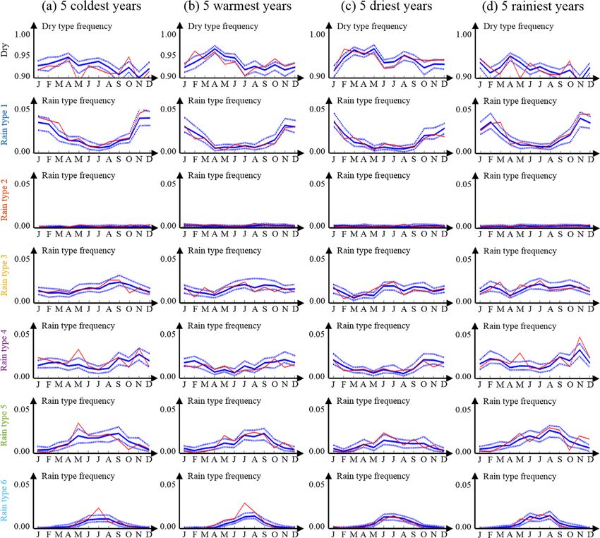
2842                         L. Benoit et al.: Nonstationary stochastic rain type generation: accounting for climate drivers

prior to model calibration) the time periods during which            shown to improve the realism of the resulting high-resolution
stationarity is assumed. Afterwards, a piecewise-stationary          space–time simulations (Benoit et al., 2018b).
modeling is applied; i.e., model parameters are kept constant           The remainder of the paper is structured as follows. First,
within a single stationary period but are allowed to vary be-        Sect. 2 presents an example of subdaily rain type time series,
tween stationary periods. The temporal scale at which non-           and Sect. 3 proposes a stochastic model able to capture the
stationarity occurs is defined by the modeler according to           main statistical features of this dataset. Next, Sect. 4 assesses
prior knowledge and assumptions about the rain process at            the performance of the model through a cross-validation pro-
hand and ranges from seasons (Paschalis et al., 2013; Bár-           cedure, and Sect. 5 illustrates the application of the pro-
dossy and Pegram, 2016; Peleg et al., 2017) to a single rain-        posed approach to the downscaling of EURO-CORDEX (Eu-
storm (Caseri et al., 2016; Benoit et al., 2018a). However,          ropean Coordinated Regional Climate Downscaling Exper-
several empirical studies have shown that at the subdaily            iment) RCM (regional climate model) precipitation future
scale, rain statistics can change at a higher rate than alleged      projections. Finally, Sect. 6 provides some conclusions about
in most piecewise-stationary stochastic rainfall models. More        stochastic rain type modeling.
precisely, rain statistics have been shown to abruptly change
within a single day (Emmanuel et al., 2012) and even within a
single rainstorm (Kumar et al, 2011; Ghada et al., 2019). To         2     Example dataset of rain type time series and related
model rain nonstationarity on a more data-driven basis and                 meteorological covariates
thereby account for the subdaily nonstationarities reported
above, it has recently been proposed to classify rain fields         Before proposing a stochastic model able to mimic the rain
into rain types (e.g., based on weather radar images) prior          type occurrence process (Sect. 3), the present section ex-
to the stochastic modeling of rain intensity (Lagrange et al.,       plains how rain type time series are derived from weather
2018; Benoit et al., 2018b). Rain fields belonging to the same       radar observations and investigates the main features of rain
rain type are then deemed statistically similar, and periods         type occurrence in a mid-latitude climate.
with a constant rain type can be regarded as stationary peri-
ods for the simulation of rain intensity.                            2.1    Rain type time series
   In this context, the main goal of this paper is to propose
a new approach to leverage the use of rain types for encod-          We focus hereafter on a 100 km × 100 km squared area cen-
ing nonstationarity in the framework of stochastic weather           tered in the city of Jena in the federal state of Thuringia, Ger-
generators. However, the finality differs from that of classi-       many (Fig. 2a). This area has been chosen because its flat
cal weather generators (Richardson, 1981; Wilks and Wilby,           topography, and its location far from coastlines or major to-
1999; Peleg et al., 2017), since we aim at simulating rain-          pographic barriers ensures spatially homogeneous rain fields,
fall conditional to meteorological covariates that are already       allowing for focusing on the temporal component of rainfall
known, instead of simulating jointly the whole weather (i.e.,        nonstationarity. Over this area, data used for rain typing con-
all variables). More precisely, we develop a method for              sist of radar images extracted from the RADOLAN (RAdar-
stochastic simulation of rain type time series conditional to        OnLine-ANeichung) dataset (Winterrath et al., 2012; Kas-
the current state of the atmosphere, i.e., conditional to mete-      par et al., 2013), which are provided in an open-access way
orological variables such as pressure, temperature, humidity         by the German meteorological agency (Deutscher Wetterdi-
or wind (Fig. 1a). These meteorological covariates are as-           enst – DWD). It consists of raw (i.e., not adjusted on rain
sumed to be known beforehand, either from observations,              gauges) radar image composites over all of Germany from
numerical weather model outputs or other stochastic simu-            1 January 2001 to present. The RADOLAN radar image res-
lations. The advantage of the proposed approach is twofold:          olution is 1 km × 1 km in space and 5 min in time. In practice,
firstly, using a stochastic simulation to generate rain types al-    however, we resampled radar images at a 10 min resolution
lows for properly reproducing the natural variability of rain        and restricted our study to the period 1 January 2001–31 De-
type occurrence and thereby to indirectly model the nonsta-          cember 2017. The RADOLAN dataset is used as baseline in-
tionarity of rain statistics observed in historical datasets. Sec-   formation for rain typing, following a space–time classifica-
ondly, the conditioning of the stochastic rain type model to         tion approach (Benoit et al., 2018b). Using raw radar images
the state of the atmosphere preserves the relationships be-          can lead to biases in estimated rain intensities, but the impact
tween rain type occurrence and climatological drivers. Once          of such biases on the classification are deemed negligible,
realistic rain type time series have been simulated (i.e., the       since the adopted approach focuses on rainfall space–time
core of this study; Fig. 1a), high-resolution rain fields can be     behavior rather than rainfall intensity. A problematic source
generated conditional to rain types using any high-resolution        of errors would be the change of radar biases along time,
stochastic rainfall generator (Vischel et al., 2011; Leblois         which could alter the interannual frequency of rain types. To
and Creutin, 2013; Paschalis et al., 2013; Nerini et al., 2017;      alleviate this problem, uniformly reprocessed radar images
Benoit et al., 2018a) as illustrated in Fig. 1b. Using rain types    are used as the basis for the classification, which ensures
to guide the stochastic generation of synthetic rains has been       a consistent data cube throughout the period of interest. In

Hydrol. Earth Syst. Sci., 24, 2841–2854, 2020                                         https://doi.org/10.5194/hess-24-2841-2020
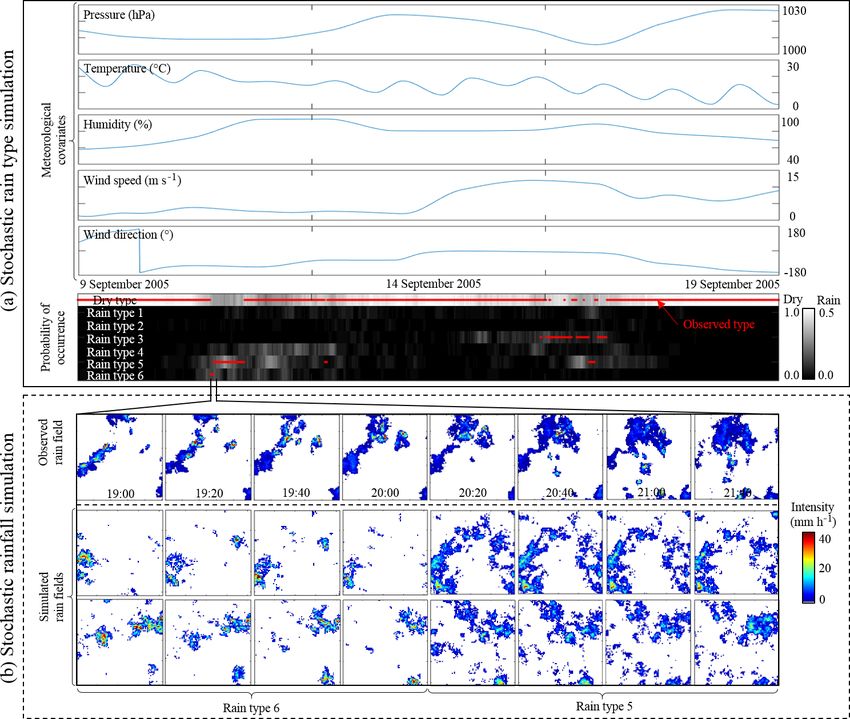
L. Benoit et al.: Nonstationary stochastic rain type generation: accounting for climate drivers                                           2843

Figure 1. Overview of stochastic rain type generation (core of this study) and its application to simulate high-resolution synthetic rain fields
whose statistical properties depend on meteorological conditions. (a) Rain type simulation framework developed in this study. (b) Illustration
of stochastic rainfall simulation conditioned to changing rain types. In the bottom row of (a), the observed rain types are in red, and the
gray-shaded background denotes the probability of rain type occurrence derived from stochastic rain type simulations conditioned to the
meteorological covariates displayed in the four top lines. In (b), the upper row displays actual rain fields observed by radar imagery, and the
two bottom rows display two stochastic simulations of synthetic rain fields for the same period generated using the approach of Benoit et al.
(2018a).

practice, no adverse trend is noted in the observed rain type             age. Among these metrics, three relate to the statistical dis-
distribution (Fig. 3).                                                    tribution of rain intensity observed in the radar image; three
   In a nutshell, the classification method proposed by Benoit            characterize the spatial arrangement of rain patterns within
et al. (2018b) and used hereafter for rain typing consists of             the image; and four evaluate the temporal evolution of the
the following. First, rainy time steps are defined as periods             rain field due to rain advection and diffusion between con-
with more than 10 % radar pixels measuring rain. The other                secutive periods. Then, the 10 metrics are used as a basis for
time steps are classified as dry and are not considered for               classification using a Gaussian mixture model (GMM). All
rain typing. For classification, 10 statistical metrics are com-          details about the 10 metrics and the clustering approach with
puted for each rainy radar image in order to assess the space–            a GMM can be found in Benoit et al. (2018b). The result-
time intensity behavior of the rain field observed in the im-             ing clusters correspond to rain fields with similar space–time

https://doi.org/10.5194/hess-24-2841-2020                                                Hydrol. Earth Syst. Sci., 24, 2841–2854, 2020
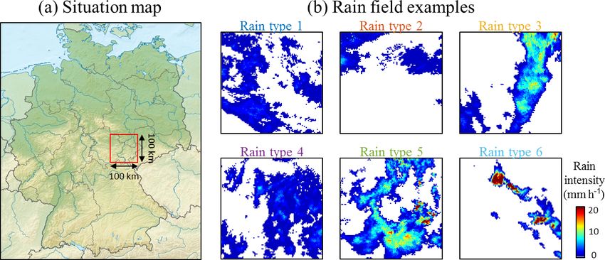
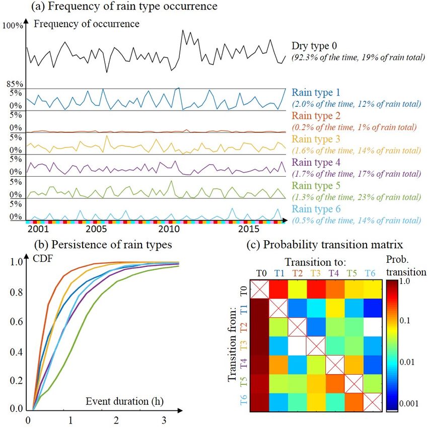
2844                          L. Benoit et al.: Nonstationary stochastic rain type generation: accounting for climate drivers

Figure 2. Radar dataset used for rain typing. (a) Study area. The red square denotes the area of interest, centered on Jena, Thuringia, Germany.
(Background map from https://www.wikipedia.org/, last access: 27 May 2020, licensed under CC BY 3.0.) (b) Example of RADOLAN radar
images (cropped over the area of interest) for each rain type.

Figure 3. Main features of a rain type time series (2001–2017) observed over central Germany. (a) Frequency of rain type occurrence
computed at a seasonal basis (seasons are December, January and February – DJF – in light blue; March, April and May – MAM – in pink;
June, July and August – JJA – in red; and September, October and November – SON – in yellow). (b) CDF of event duration stratified by
rain type. (c) Empirical matrix of transition probability between rain types.

Hydrol. Earth Syst. Sci., 24, 2841–2854, 2020                                                https://doi.org/10.5194/hess-24-2841-2020
L. Benoit et al.: Nonstationary stochastic rain type generation: accounting for climate drivers                              2845

behaviors. The number of rain types is selected as a compro-           Figure 3 investigates the occurrence of rain types through
mise between the goodness of fit to rain field statistics and       time and highlights some features. Figure 3a displays the fre-
model parsimony. In the present case, the parsimony is fa-          quency of each rain type at the seasonal scale. It appears
vored in order to allow for a physical interpretation of the        from Fig. 3a that the frequency of occurrence of individual
resulting rain types. As a result, six rain types are identified    rain types is strongly variable across the year. For example,
in the example dataset (Fig. 2b). Among them, rain types 1          stratiform rain types 1 and 4 occur mostly in winter, while
and 4 correspond to rather stratiform and spread rain events;       convective rain types 5 and 6 are most common in summer.
rain type 3 corresponds to frontal rainstorms; and rain types 5     In addition, one can notice a strong interannual variability in
and 6 can be associated with rather convective rains. Rain          rain occurrence, with summers 2003 and 2011 having a low
type 2 cannot be associated to a specific rain behavior but         occurrence of rain, while rain occurrence is particularly high
rather gathers rain fields that are not classified otherwise and    during winters 2006 and 2011. Figure 3b displays the cumu-
often correspond to partial rain coverage.                          lative distribution function (CDF) of the duration of each rain
   Using only radar images with more than 10 % wet pixels           type. Here rain type duration is defined as the duration (i.e.,
to define rain types ensures a reliable classification but at the   length along the time axis) of a segment of constant rain type.
cost of a dry bias (in the present dataset, 32 % of the im-         Each curve in Fig. 3b therefore corresponds to the probability
ages have a rain fraction between 0 % and 10 % and encom-           that a rain event of a given type does not exceed the duration
pass 19 % of the rain total; cf. Fig. 3). To deal with images       given in abscissa. This figure shows that all rain types are
with less than 10 % wet pixels, Benoit et al. (2018b) proposed      persistent in time with durations ranging from a few minutes
classifying images with a small rain fraction (i.e., 0 % < rain     to more than 3 h and that some types (e.g., rain types 4 and 5)
fraction < 10 %) in a second step by assigning them the type        are more persistent than others (e.g., rain types 2 and 3).
of the closest classified image (i.e., nearest neighbor inter-      Finally, Fig. 3c displays the empirical transition matrix be-
polation in time). This postprocessing scheme is not directly       tween rain types and focuses on inter-type transitions (i.e.,
transferable to the context of simulation because no informa-       transitions to the same type are ignored and denoted by red
tion about images with low rain coverage is available in sim-       crosses). This figure shows that the patterns of transition be-
ulation outputs. Two options can be considered to alleviate         tween rain types are complex and that the transitions involv-
this problem. First, the rain type model defined in Sect. 3 can     ing type 0 (i.e., no rain) are largely dominant.
be calibrated on the final classification (i.e., including images
with low rain coverage), which results in simulations that          2.2   Meteorological covariates
preserve the actual rain proportion. However, using a clas-
sification that includes the onset and the end of rainstorms        The strong seasonality and interannual variability of rain type
leads to less clear relationships between climate covariates        occurrence emerging from Fig. 3a can be explained to a large
and rain type occurrence, which may degrade simulation re-          extent by regional meteorological conditions. Hereafter, we
sults. Hence the second option, which we follow in this pa-         investigate the links between rain type occurrence and a set
per, which consists of (1) calibrating and running the rain         of five meteorological covariates that are deemed to influ-
type model for rain types defined only from radar images            ence rainfall behavior (Vrac et al., 2007; Willems, 2001; Rust
with more than 10 % rain coverage and then (2) readjusting          et al., 2013), namely sea level pressure, temperature at 2 m,
the dry–wet balance by postprocessing. The dry bias is cor-         relative humidity, and the direction and intensity of synop-
rected assuming the ratio R = N     s
                                  Nl between the number Ns of       tic wind at 850 hPa. The actual values of the meteorological
images with low rain coverage and the number Nl of images           covariates used in this study are extracted from the ERA5 re-
with large rain coverage as a constant in observations and          analyzes (Hersbach et al., 2018) and averaged over the whole
simulations. Subsequently, the number of epochs for which           area of interest before further use. Only parameters provided
rain is simulated is increased by propagating the closest rain      at daily resolution are used hereafter in order to be compat-
type to the R × Nl dry epochs located at the beginning and at       ible with the temporal resolution of RCM projections used
the end of rainstorms. Section S1 in the Supplement shows           for the illustration of our framework (see Sect. 5). To match
that such postprocessing performs well to mitigate the dry          the resolution of rain type data, the above daily resolution
bias originating from the use of a 10 % rain coverage thresh-       meteorological covariates are disaggregated to a 10 min res-
old to define a wet image. However, since the present study         olution. To this end, the mean daily pressure, humidity, wind
focuses on climate–rain-type relationships, which are better        direction and wind intensity are assumed to occur at 00:00 LT
defined when considering only the first step of the classifi-       (local time) and are then interpolated at a 10 min resolution
cation, the aforementioned postprocessing is not applied in         using a polynomial interpolation. For temperature, the daily
the remainder of this paper. Hence, one should keep in mind         minimum is assumed to occur at 05:00 LT, and the daily max-
that in the following the dry type also includes epochs with a      imum is assumed to occur at 15:00 LT; the diurnal cycle is
low rain coverage (under 10 %) and that postprocessing is re-       captured by spline interpolation. This disaggregation frame-
quired if the end-use application involves the stochastic sim-      work leads to 10 min resolution meteorological covariates in
ulation of actual rain fields.                                      good agreement with actual 10 min resolution observations

https://doi.org/10.5194/hess-24-2841-2020                                        Hydrol. Earth Syst. Sci., 24, 2841–2854, 2020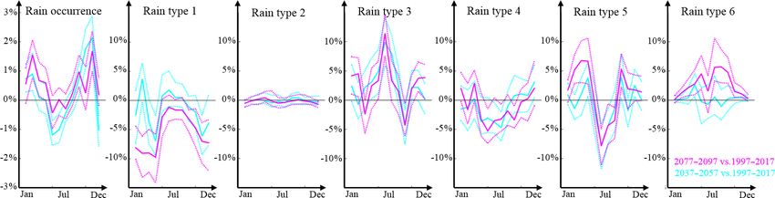
2846                          L. Benoit et al.: Nonstationary stochastic rain type generation: accounting for climate drivers

Figure 4. Statistics of meteorological covariates for each rain type. The meteorological data were extracted from the ERA5 reanalysis dataset.

carried out by a weather station located close to the center of          combine both frameworks to build a nonhomogeneous semi-
the area of interest, and rain type simulations conditioned to           Markov model. Unfortunately, semi-Markov models do not
these two sets of covariates (in situ observations and disag-            allow for an easy conditioning to continuous-time covariates,
gregated reanalysis data) give very similar results (Sect. S2;           and our attempt to build a nonhomogeneous semi-Markov
Fig. S3).                                                                model led to a significant dry bias in rain type simulations
   Figure 4 displays the relationships between meteorolog-               (Sect. S3). Hence, it appeared that even relatively sophisti-
ical covariates and rain type occurrence and confirms the                cated parametric models are challenged by the complexity of
strong influence of temperature and wind speed on rain types.            rainfall at subdaily resolution (Oriani et al., 2018).
Indeed, stratiform rain types 1 and 4 occur at lower tem-                   One alternative to account for such complexity is to
peratures than convective types 5 and 6 and co-occur with                consider high-order properties through a nonparametric ap-
stronger winds. The frontal rain type 3 is characterized by              proach based on the resampling of historical datasets (Oriani
strong westerlies but occurs for a broad range of tempera-               et al., 2014). For the simulation of rain types conditional to
tures. In contrast to temperature and wind speed, the stan-              meteorological covariates, we therefore adopt the framework
dalone knowledge of pressure, relative humidity or wind di-              of a multiple-point simulation (MPS). MPS consists of us-
rection does not allow for discriminating between all rain               ing a training dataset (here a past rain type record) to esti-
types. However, when considered jointly (Sect. S2; Fig. S4),             mate empirically the probability distribution of the variable
all meteorological covariates bring information about rain               of interest (here rain type occurrence at a given time step)
type occurrence. In particular, pressure and humidity are key            conditionally to the values already simulated in its tempo-
drivers for rain occurrence (no matter the type) and are there-          ral neighborhood (Fig. 5a). In the specific MPS algorithm
fore useful to predict dry and wet spells. Furthermore, wind             we use (Gravey and Mariethoz, 2018, 2019), the conditional
direction informs the occurrence of rain type 3 and helps to             probability density function (PDF) is indirectly assessed by
discriminate between rain types 5 and 6.                                 making a random sampling of the training dataset that aims
                                                                         at finding a pattern that is similar to the local conditioning
                                                                         neighborhood (Fig. 5b). In practice, we use a 100 h neighbor-
3   Stochastic rain type model                                           hood for the present application. Once a match is found (i.e.,
                                                                         a pattern in the training image that minimizes the Hamming
Daily resolution stochastic weather generators do not dis-
                                                                         distance with the target pattern), the corresponding value is
tinguish between rain types and typically resort to Markov
                                                                         imported in the simulation grid (Fig. 5c), and the procedure
chain models to simulate rain occurrence (Richardson, 1981;
                                                                         is iterated until the full simulation grid is filled. In the MPS
Wilby, 1994; Wilks and Wilby, 1999). Within Markov chain
                                                                         framework, the dependence of rain type occurrence to me-
models, semi-Markov models are often favored when the
                                                                         teorological covariates can be handled by multivariate-MPS
persistence of dry and wet spells is of prime importance
                                                                         simulation (Mariethoz et al., 2010). It consists of stacking
(Foufoula-Georgiou and Lettenmaier, 1987; Bárdossy and
                                                                         time series of meteorological covariates with the time se-
Plate, 1991), and nonhomogeneous Markov models are pre-
                                                                         ries of rain type occurrence and evaluating the conditioning
ferred when the dry–wet sequence has to be conditioned to
                                                                         neighborhood on the time series of the resulting vector vari-
meteorological covariates (Hughes and Guttorp, 1999; Vrac
                                                                         able. Here we use a simplified version of a multivariate-MPS
et al., 2007). An easy option to deal with rain type simulation
                                                                         simulation where only the co-located covariates (i.e., the val-
conditional to meteorological covariates would therefore be
                                                                         ues of the covariates observed at the exact time step to simu-
to extend one of these Markov-chain-based frameworks by
                                                                         late) are accounted for during the matching procedure.
simply increasing the number of states of the Markov chain
                                                                            Since MPS is a nonparametric approach, it does not re-
in order to account for the diversity of rain types. However,
                                                                         quire model calibration strictly speaking. Instead, it requires
both rain type persistence and conditioning to covariates are
                                                                         a training dataset to resample, which should include both the
equally important for the targeted application, which led us to

Hydrol. Earth Syst. Sci., 24, 2841–2854, 2020                                               https://doi.org/10.5194/hess-24-2841-2020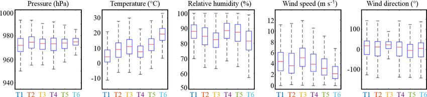
L. Benoit et al.: Nonstationary stochastic rain type generation: accounting for climate drivers 2847
Figure 5. Schematic view of the MPS algorithm used for the nonparametric resampling of historical rain type time series.
variable of interest (here a rain type time series) and optional typical features of rain type occurrence highlighted in Sect. 2,
covariates (here meteorological covariates). To produce re- namely seasonality, persistence and transition. Figure 6a as-
liable results and, in particular, meaningful uncertainty esti- sesses rain type seasonality and shows that for strongly sea-
mates, MPS requires large training datasets (Emery and Lan- sonal rain types (types 1, 5 and 6) the annual cycle of rain
tuéjoul, 2014). In the present case, the training dataset is the type occurrence is properly simulated. It is also worth noting
historical record of joint rain types and meteorological co- that the interannual variability of the annual cycle is reason-
variates observations available over the target area (17 years). ably well simulated, as well as the interannual variability of
After the selection of a training dataset, simulations are ob- weakly seasonal rain types (types 3 and 4). This shows that
tained by resampling the training dataset using the MPS al- the proposed approach not only reproduces the annual cycle
gorithm described above. of rain type occurrence driven by monthly scale variations of
the covariates but also captures the impact of short-term fluc-
tuations of meteorological conditions that trigger rainstorms
4 Model assessment of types 3 and 4. However, when scrutinizing the minima
and maxima in Fig. 6a, one can notice that peaks in obser-
4.1 Cross-validation procedure vations are smoothed out in simulations, which traduces the
difficulty of the model to simulate extreme cases. This is a
Model performance is assessed by a cross-validation proce-
known drawback of MPS simulations (Mariethoz and Caers,
dure, using the dataset introduced in Sect. 2. In practice, we
2015), and it constitutes the main limitation of the present ap-
adopt a procedure of leaving 1 year out. For a given sim-
proach for the simulation of future climates in which unusual
ulation year, the rain type model is first trained using data
climatic conditions are deemed to become more frequent.
from the 2001–2017 period, excluding the year to simulate.
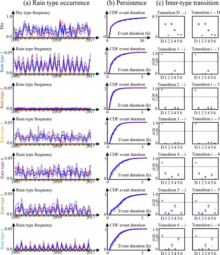
Regarding rain type persistence, Fig. 6b shows that this fea-
Next, 50 realizations of rain type time series are generated
ture is in general very well reproduced, except for the long-
for the year of interest by MPS simulation and conditioned
lasting types 4 and 5, for which persistence is slightly un-
to observations of the meteorological covariates derived from
derestimated. Finally Fig. 6c assesses inter-type transitions.
the ERA5 reanalysis as described in Sect. 2. Finally, the
One can notice that the transition patterns are almost per-
same procedure is iterated for each year of the test period
fectly reproduced, except for the transition from dry (and to
(i.e., 2001–2017), and 50 realizations of 17-year-long rain
a lesser extent from type 5) to rain type 6 that is underesti-
type time series are obtained by concatenating in time the
mated (overestimated, respectively).
17 yearly simulations.
Overall, the proposed stochastic rain type model properly
The 50 simulations are compared to the reference rain type
reproduces the main features of observed rain type time se-
time series in Fig. 6. Focusing first on the ability of the model
ries. This good performance is linked to the ability of MPS
to simulate dry and wet conditions (i.e., without distinction
to accurately reproduce high-order statistics of rain type time
between rain types), the first panel of Fig. 6a compares the
series.
observed and simulated frequencies of dry occurrence for
each season of the validation period 2001–2017. The results
show that our model properly simulates the overall propor- 4.2 Sensitivity to climate variability
tion of rain (ratio of simulated to observed rain frequency
is 0.93). In addition, the chronology of dry–wet occurrence To ensure that the proposed rain type model is able to cap-
at the seasonal scale is reasonably simulated (correlation be- ture the impact of climatic signals on rain type occurrence,
tween observed and simulated dry type occurrence is 0.6). the results of the cross-validation procedure are stratified ac-
Focusing next on the simulation of rain types, Fig. 6 cording to annual climatic signatures. To this end, Fig. 7
(lines 2–7) assesses the ability of the model to reproduce the compares simulated and observed rain type occurrences at
https://doi.org/10.5194/hess-24-2841-2020 Hydrol. Earth Syst. Sci., 24, 2841–2854, 20202848 L. Benoit et al.: Nonstationary stochastic rain type generation: accounting for climate drivers Figure 6. Results of the cross-validation experiment. (a) Seasonality of rain (and dry) type occurrence (seasons are DJF in light blue, MAM in pink, JJA in red and SON in yellow), (b) rain type persistence and (c) probability of transition between rain types. Observations are in red, and simulations are in blue. In simulations, continuous lines represent the median of the simulated ensembles (50 realizations), and dashed lines represent the Q10 and Q90 quantiles. Hydrol. Earth Syst. Sci., 24, 2841–2854, 2020 https://doi.org/10.5194/hess-24-2841-2020
L. Benoit et al.: Nonstationary stochastic rain type generation: accounting for climate drivers                                2849

the monthly scale for four sub-datasets: the 5 coldest years        centration Pathway) emission scenario. Three intervals of 20
of the 2001–2017 period (Fig. 7a), the 5 warmest years              years each are selected to investigate the evolution of rain
(Fig. 7b), the 5 driest years (Fig. 7c) and finally the 5 wettest   type occurrence over the 21st century: 1997–2017 (reference
years (Fig. 7d). Observations (red curves in Fig. 7) show that      period that encompasses the 2001–2017 calibration period
years with different climatic signatures indeed develop dis-        for which rain type observations are available), 2037–2057
tinct dry / wet ratios and rain type distributions. Simulation      and 2077–2097. For each period, the meteorological covari-
results (blue curves in Fig. 7) show that the proposed model        ates are extracted from the RCM simulation, averaged over
properly reproduces these climatically driven differences in        the area of interest and disaggregated at a 10 min resolution
rain type distribution.                                             as described in Sect. 2. In addition, RCM outputs are bias-
   Figure 7 therefore allows for a detailed investigation of        corrected using the CDF-t (cumulative distribution function
the impact of climatic signals on local rain type distribution      transform) method for each variable separately (Vrac et al.,
over central Germany. Comparing first cold and warm years           2012). After the bias correction of RCM data, the perfor-
(Fig. 7a and b), one can notice that warm years tend to be          mance of the model to simulate rain types in the present
drier, in particular in late winter and spring. This is mostly      climate is almost identical for meteorological covariates de-
caused by a deficit of type 1 precipitation during warm years,      rived from the RACMO-KNMI RCM and the ones derived
which corresponds to less snow (type 1 occurs mostly at low         from the ERA5 reanalysis (Sect. S4).
temperatures; cf. Fig. 4). Drier springs during warm years             For each 20-year period, 50 realizations are simulated con-
are also caused by a deficit of type 5 (slightly convective),       ditional to bias-corrected RCM-derived meteorological co-
which probably corresponds for this time of the year to rain        variates. To evaluate the projected changes in rain type distri-
and sleet showers. Finally, one can notice an increased oc-         bution, Fig. 8 displays the evolution of the monthly frequency
currence of type 6 (strongly convective) during warm years,         of rain type occurrence between the reference period 1997–
which is captured by the model despite a slight underesti-          2017 and the two future periods 2037–2057 and 2077–2097.
mation of this type for both cold and warm years. Compar-           Observed changes in rain type occurrence frequency are con-
ing dry and wet years (Fig. 7c and d), one can notice that          sidered as significant if they exceed the uncertainty of the
all months contribute to the rain imbalance but that the rain       projection that is defined as the Q10 –Q90 interval of the
deficit is more pronounced in spring and autumn. In terms           50 realizations. It should be noted that in contrast to rain type
of rain type distribution, this is mostly caused by a deficit       occurrence, the simulated persistence and transition behav-
of rain types 1 and 4 (stratiform) as well as 5 (slightly con-      ior of rain types remain constant over the whole test period
vective) during dry years. It is also worth noting that rain        (not shown). Results in Fig. 8 show that the frequency of
type 3 (frontal) tends to be slightly more common during            rain occurrence slightly decreases in summer and increases
rainy years, but in contrast to other types, its increased oc-      in winter, spring and autumn. Among these changes, only
currence is spread along the whole year.                            the increase of rain occurrence during autumn and winter is
   Overall, the proposed approach properly captures the im-         significant. The distribution of rain types conditional to the
pact of climatic signals on rain type occurrence. This prop-        presence of rain is more significantly modified than rain oc-
erty is essential to preserve the relationships between rain        currence. More precisely, during winter, rain type 1 (strat-
types and climatological drivers and paves the way to RCM           iform) significantly declines, while the frequency of rain
precipitation downscaling.                                          types 3 (frontal) and 5 (moderately convective) significantly
                                                                    increases. During spring and autumn, rain type 1 (stratiform)
                                                                    significantly declines, while rain types 5 and 6 (convective)
5   Application to RCM precipitation downscaling                    tend to increase but not significantly. Finally, during summer,
                                                                    rain types 1, 4 (stratiform) and 5 (moderately convective) de-
For illustration purposes, the stochastic rain type model de-       crease, while rain types 3 (frontal) and 6 (strongly convec-
veloped in Sect. 3 is used to simulate the evolution of             tive) increase, with most of these changes being significant.
rain type occurrence in a changing climate simulated by             Overall, it appears from this exploratory study that under the
one RCM run extracted from the EURO-CORDEX climate                  assumption of the specific RCM run used to simulate the me-
downscaling experiment (Jacob et al., 2014). To drive the           teorological covariates, convective and frontal rains could be-
simulation of rain types in a changing climate, the same set        come more frequent at the expense of stratiform rains by the
of meteorological covariates as the one used in the cross-          end of the 21st century. The most significant changes are ob-
validation procedure is derived from one RCM run, more pre-         tained during winter and summer. It is worth mentioning that
cisely from the Regional Atmospheric Climate MOdel of the           the evolution of rain behavior along the 21st century sim-
Dutch national weather service (RACMO-KNMI; Van Mei-                ulated in the present study is qualitatively in line with re-
jgaard et al., 2008) driven by the CNRM-CM5 (Centre Na-             sults obtained over western Europe by studies using physical
tional de Recherches Météorologiques Coupled global cli-            models, which anticipate more frequent heavy rains driven
mate Model, version 5) Earth system model (Voldoire et al.,         by convection or active fronts (Molnar et al., 2013; Faranda
2013) forced according to the RCP8.5 (Representative Con-

https://doi.org/10.5194/hess-24-2841-2020                                        Hydrol. Earth Syst. Sci., 24, 2841–2854, 2020
2850 L. Benoit et al.: Nonstationary stochastic rain type generation: accounting for climate drivers
Figure 7. Monthly rain type occurrence stratified according to climate forcing: (a) 5 coldest years of the 2001–2017 period (2001, 2004,
2005, 2010 and 2013), (b) 5 warmest years (2007, 2011, 2014, 2015 and 2017), (c) 5 driest years (2003, 2011, 2012, 2015 and 2016) and
(d) 5 wettest years (2001, 2002, 2007, 2009 and 2010). Observations are in red, and simulations are in blue. In simulations, continuous lines
represent the median of the simulated ensembles (50 realizations), and dashed lines represent the Q10 and Q90 quantiles.
et al., 2019) at the expense of low-intensity stratiform pre- are simulated conditional to meteorological covariates to ac-
cipitations. count for the diversity of rainstorms at the regional scale.
This first step is the main focus of the present paper. For sub-
sequent applications, we assume that the rain intensity can
6 Concluding remarks be simulated conditional to rain types. This is the classical
aim of space–time-distributed stochastic rainfall generators,
6.1 Discussion
which are becoming more and more common to address the
By introducing a step of rain type simulation in the frame- needs of high-resolution hydrometeorological impact studies
work of stochastic rainfall generators, we suggest that for (Vischel et al., 2011; Leblois and Creutin, 2013; Paschalis
high-temporal-resolution applications, the simulation of rain et al., 2013; Nerini et al., 2017; Benoit et al., 2018a).
can be split in two steps (Fig. 1). In a first instance, rain types
Hydrol. Earth Syst. Sci., 24, 2841–2854, 2020 https://doi.org/10.5194/hess-24-2841-2020L. Benoit et al.: Nonstationary stochastic rain type generation: accounting for climate drivers 2851
Figure 8. Changes in rain occurrence frequency (left panel) and rain type distribution conditional to the presence of rain (other panels)
simulated using the stochastic rain type model developed in Sect. 3: 2037–2057 vs. 1997–2017 (light blue) and 2077–2097 vs. 1997–
2017 (purple). Continuous lines represent the median of the simulated ensembles (50 realizations), and dashed lines represent the Q10 and
Q90 quantiles.
Hence, two main applications can be considered for that enough observations are available to calibrate the rain in-
stochastic rain type simulation. The first one, briefly illus- tensity model for each rain type and therefore prevents model
trated in Sect. 5, consists of assessing the evolution of the sta- overfitting. The second advantage is the added flexibility to
tistical signature of rainfall in a changing climate simulated simulate rainstorm dynamics, which allows for generating
by RCMs. It is worth noting that if one wants to carefully intra-storm variations of the space–time rainfall statistics.
evaluate the change in rain type occurrence that may emerge
in the future, one should rely on a large ensemble of emis-
6.2 Outlook
sion scenario, general circulation model and regional climate
model combinations to properly capture the uncertainty on
meteorological covariates. In addition, one should keep in In this paper, a nonparametric approach based on the resam-
mind that the present approach only accounts for changes in pling of historical records using multiple-point statistics has
the distribution of existing rain types and therefore ignores been proposed and thoroughly tested for the simulation of
the possible emergence of new rain types in response to cli- rain type time series conditional to meteorological covari-
mate conditions that have never been observed over the area ates. Evaluation results based on a 17-year-long rain type
of interest. Such new rain types could potentially be mod- dataset in a mid-latitude climate (central Germany) show that
eled by reparametrizing the stochastic rainfall model used to MPS simulations are able to reproduce both the internal vari-
simulate local rain fields (Peleg et al., 2019), by using rain ability of rain type time series, as well as relationships with
analogs from areas that today experience the climate that is meteorological covariates. After validation, stochastic rain
simulated in the future over the area of interest (Hallegatte type simulation is applied to the downscaling of RCM pro-
et al., 2007; Fitzpatrick and Dunn, 2019) or by running a jections over the 21st century. Rain type simulations condi-
convection-permitting climate model (Prein et al., 2015) for tioned to meteorological covariates simulated by a regional
the newly emerging climate conditions. The development of climate model under an RCP8.5 emission scenario indicate
a framework to model emerging rain types is however left for a possible change in rain type distribution by the end of the
future research. century, with an increased frequency of heavy rains driven
The second application is the simulation of rain intensity by convection or active fronts, and a decline of low-intensity
at high space–time resolution while preserving consistency stratiform precipitations.
with climatological drivers such as temperature, pressure, hu- The ability of stochastic simulations to generate realistic
midity and wind. As mentioned in the Introduction, simu- rain type time series when conditioned to meteorological co-
lating rain intensity would require setting up and calibrat- variates advocates for including stochastic rain type simu-
ing a high-resolution stochastic rainfall model for each rain lation into rainfall generators in order to (1) reproduce the
type over the area of interest and was therefore not consid- internal variability or rain type occurrence, in particular in-
ered in the present study except in Fig. 1b for illustration terannual variability, seasonality, persistence and inter-type
purposes. However, two advantages are expected to emerge transitions, and (2) preserve the relationships between rain
from adding a rain type simulation step into stochastic rain- statistics and meteorological covariates, in the present case
fall modeling: first, a relatively low number of rain types can temperature, pressure, humidity and wind. The above fea-
be specified, which implies that the model of rain intensity tures make stochastic rain type simulation a convenient tool
has to be calibrated a limited number of times. This ensures to account for the nonstationarity of rain statistics driven by
meteorological conditions. This opens the door to the sub-
https://doi.org/10.5194/hess-24-2841-2020 Hydrol. Earth Syst. Sci., 24, 2841–2854, 20202852 L. Benoit et al.: Nonstationary stochastic rain type generation: accounting for climate drivers
daily stochastic downscaling of climate projections and to Benoit, L.: Rain type data over Thuringia for the period 2001–
improved stochastic rainfall simulations. 2017, available at: https://github.com/LionelBenoit/Stochastic_
Raintype_Generator/Raintype_data (last access: 27 May 2020),
2020a.
Code and data availability. All data and codes used in this study Benoit, L.: Rain typing software, available at: https://github.com/
are open source and freely available in the following repositories: LionelBenoit/Rain_typing (last access: 27 May 2020), 2020b.
Benoit, L.: Stochastic rainfall generator software, available
– radar data at https://opendata.dwd.de/climate_environment/ at: https://github.com/LionelBenoit/Stochastic_Raintype_
CDC/grids_germany/5_minutes/radolan (last access: Generator/codes (last access: 27 May 2020), 2020c.
27 May 2020) (DWD, 2020) Benoit, L., Allard, D., and Mariethoz, G.: Stochastic Rainfall Mod-
– rain type data at https://github.com/LionelBenoit/Stochastic_ elling at Sub-Kilometer Scale, Water Resour. Res., 54, 4108–
Raintype_Generator/Raintype_data (last access: 27 May 2020) 4130, https://doi.org/10.1029/2018WR022817, 2018a.
(Benoit, 2020a) Benoit, L., Vrac, M., and Mariethoz, G.: Dealing with non-
stationarity in sub-daily stochastic rainfall models, Hydrol. Earth
– rain typing software at https://github.com/LionelBenoit/Rain_
Syst. Sci., 22, 5919–5933, https://doi.org/10.5194/hess-22-5919-
typing (last access: 27 May 2020) (Benoit, 2020b)
2018, 2018b.
– stochastic rain type models at https://github.com/ Burton, A., Fowler, H. J., Blenkinsop, S., and Kilsby, C. G.: Down-
LionelBenoit/Stochastic_Raintype_Generator/codes (last scaling transient climate change using a Neyman–Scott Rectan-
access: 27 May 2020) (Benoit, 2020c) gular Pulses stochastic rainfall model, J. Hydrol., 381, 18–32,
– MPS simulation software at https://github.com/GAIA-UNIL/ https://doi.org/10.1016/j.jhydrol.2009.10.031, 2010.
G2S (last access: 27 May 2020) (Gravey, 2020). Caseri, A., Javelle, P., Ramos, M. H., and Leblois, E.:
Generating precipitation ensembles for flood alert and
risk management, J. Flood Risk Manage., 9, 402–415,
Supplement. The supplement related to this article is available on- https://doi.org/10.1111/jfr3.12203, 2016.
line at: https://doi.org/10.5194/hess-24-2841-2020-supplement. DWD – Deutcher Wetterdienst: Radolan radar products, available
at: https://opendata.dwd.de/climate_environment/CDC/grids_
germany/5_minutes/radolan, last access: 27 May 2020.
Emery, X. and Lantuéjoul, C.: TBSIM: A computer program for
Author contributions. LB, MV and GM designed the study. LB per-
conditional simulation of three-dimensional Gaussian random
formed the numerical experiments. LB wrote the paper with input
fields via the turning bands method, Comput. Geosci., 32, 1615–
and corrections from MV and GM.
1628, https://doi.org/10.1016/j.cageo.2006.03.001, 2014.
Emmanuel, I., Andrieu, H., Leblois, E., and Flahaut, B.:
Temporal and spatial variability of rainfall at the ur-
Competing interests. The authors declare that they have no conflict ban hydrological scale, J. Hydrol., 430–431, 162–172,
of interests. https://doi.org/10.1016/j.jhydrol.2012.02.013, 2012.
Faranda, D., Alvarez-Castro, C., Messori, G., Rodrigues, D., and
Yiou, P.: The hammam effect or how a warm ocean enhances
Acknowledgements. The authors are grateful to the editor and to the large scale atmospheric predictability, Nat. Commun., 10, 1316,
three reviewers for their comments and suggestions. https://doi.org/10.1038/s41467-019-09305-8, 2019.
Fitzpatrick, M. C. and Dunn, R. R.: Contemporary climatic analogs
for 540 North American urban areas in the late 21st century, Nat.
Review statement. This paper was edited by Nadav Peleg and re- Commun., 10, 614, https://doi.org/10.1038/s41467-019-08540-
viewed by András Bárdossy, Hjalte Jomo Danielsen Sørup, and one 3, 2019.
anonymous referee. Foufoula-Georgiou, E. and Lettenmaier, D.: A Markov Renewal
Model for Rainfall Occurence, Water Resour. Res., 23, 875–884,
https://doi.org/10.1029/WR023i005p00875, 1987.
Furrer, E. M. and Katz, R. W.: Generalized linear modeling ap-
References proach to stochastic weather generators, Clim. Res., 34, 129–
144, https://doi.org/10.3354/cr034129, 2007.
Ailliot, P., Allard, D., Monbet, V., and Naveau, P.: Stochastic Ghada, W., Estrella, N., and Menzel, A.: Machine Learn-
weather generators: an overview of weather type models, Jour- ing Approach to Classify Rain Type Based on Thies Dis-
nal de la société française de statistiques, 156, 101–113, 2015. drometers and Cloud Observations, Atmosphere, 10, 251,
Bárdossy, A. and Pegram, G. G. S.: Space-time condi- https://doi.org/10.3390/atmos10050251, 2019.
tional disaggregation of precipitation at high resolu- Gires, A., Tchiguirinskaia, I., Schertzer, D., Schellart, A.,
tion via simulation, Water Resour. Res., 52, 920–937, Berne, A., and Lovejoy, S.: Influence of small scale
https://doi.org/10.1002/2015WR018037, 2016. rainfall variability on standard comparison tools between
Bárdossy, A. and Plate, E. J.: Modelling daily rainfall using a semi- radar and rain gauge data, Atmos. Res., 138, 125–138,
Markov representation of circulation pattern occurence, J. Hy- https://doi.org/10.1016/j.atmosres.2013.11.008, 2014.
drol., 122, 33–47, https://doi.org/10.1016/0022-1694(91)90170-
M, 1991.
Hydrol. Earth Syst. Sci., 24, 2841–2854, 2020 https://doi.org/10.5194/hess-24-2841-2020L. Benoit et al.: Nonstationary stochastic rain type generation: accounting for climate drivers 2853 Gravey, M.: G2S: The GeoStatistical Server, available at: https:// the turning band method, Water Resour. Res., 49, 3375–3387, github.com/GAIA-UNIL/G2S, last access: 27 May 2020. https://doi.org/10.1002/wrcr.20190, 2013. Gravey, M. and Mariethoz, G.: Quantile Sampling: a new approach Mariethoz, G. and Caers, J.: Multiple-Point Geostatistics: Stochas- for multiple-point statistics simulation, in: IAMG 2018 Confer- tic Modeling with Training Images, Wiley Blackwell, Hoboken, ence, Olomouc, Czech Republic, 2018. USA, 364 pp., 2015. Gravey, M. and Mariethoz, G.: Quantile Sampling: a robust Mariethoz, G., Renard, P., and Straubhaar, J.: The Di- and simplified pixel-based multiple-point simulation approach, rect Sampling method to perform multiple-point geo- Geosci. Model Dev. Discuss., https://doi.org/10.5194/gmd-2019- statistical simulations, Water Resour. Res., 46, W11536, 211, in review, 2019. https://doi.org/10.1029/2008WR007621, 2010. Hallegatte, S., Hourcade, J. C., and Ambrosi, P.: Using cli- Marra, F. and Morin, E.: Autocorrelation structure of con- mate analogues for assessing climate change economic vective rainfall in semiarid-arid climate derived from high- impacts in urban areas, Climatic Change, 82, 47–60, resolution X-Band radar estimates, Atmos. Res., 200, 126–138, https://doi.org/10.1007/s10584-006-9161-z, 2007. https://doi.org/10.1016/j.atmosres.2017.09.020, 2018. Hersbach, H., de Rosnay, P., Bell, B., Schepers, D., Simmons, Mascaro, G., Deidda, R., and Hellies, M.: On the nature of A., Soci, C., Abdalla, S., Alonso-Balmaseda, M., Balsamo, G., rainfall intermittency as revealed by different metrics and Bechtold, P., Berrisford, P., Bidlot, J.-R., de Boisséson, E., sampling approaches, Hydrol. Earth Syst. Sci., 17, 355–369, Bonavita, M., Browne, P., Buizza, R., Dahlgren, P., Dee, D., Dra- https://doi.org/10.5194/hess-17-355-2013, 2013. gani, R., Diamantakis, M., Flemming, J., Forbes, R., Geer, A. Mavromatis, T. and Hansen, J. W.: Interannual variability char- J., Haiden, T., Hólm, E., Haimberger, L., Hogan, R., Horányi, acteristics and simulated crop response of four stochastic A., Janiskova, M., Laloyaux, P., Lopez, P., Munoz-Sabater, J., weather generators, Agr. Forest Meteorol., 109, 283–296, Peubey, C., Radu, R., Richardson, D., Thŕpaut, J.-N., Vitart, F., https://doi.org/10.1016/S0168-1923(01)00272-6, 2001. Yang, X., Zsótér, E., and Zuo, H.: Operational global reanaly- Molnar, P., Fatichi, S., Gaàl, L., Szolgay, J., and Burlando, P.: sis: progress, future directions and synergies with NWPRep, in: Storm type effects on super Clausius–Clapeyron scaling of in- ERA Report Series, ECMWF report, ECMWF, Reading, Eng- tense rainstorm properties with air temperature, Hydrol. Earth land, 2018. Syst. Sci., 19, 1753–1766, https://doi.org/10.5194/hess-19-1753- Hughes, J. P. and Guttorp, P.: A non-homogeneous hidden Markov 2015, 2013. model for precipitation occurence, Appl. Stat., 48, 15–30, Nerini, D., Besic, N., Sideris, I. V., Germann, U., and Foresti, L.: https://doi.org/10.1111/1467-9876.00136, 1999. A non-stationary stochastic ensemble generator for radar rainfall Jacob, D., Petersen, J., Eggert, B., Alias, A., Bøssing Chris- fields based on the short-space Fourier transform, Hydrol. Earth tensen, O., Bouwer, L. M., Braun, A., Colette, A., Déqué, Syst. Sci., 21, 2777–2797, https://doi.org/10.5194/hess-21-2777- M., Georgievski, G., Georgopoulou, E., Gobiet, A., Menut, L., 2017, 2017. Nikulin, G., Haensler, A., Hempelmann, N., Jones, C., Keuler, Oriani, F., Mehrotra, R., Mariethoz, G., Straubhaar, J., Sharma, A., K., Kovats, S., Kröner, N., Kotlarski, S., Kriegsmann, A., Mar- and Renard, P.: Simulation of rainfall time series from differ- tin, E., van Meijgaard, E., Moseley, C., Pfeifer, S., Preuschmann, ent climatic regions using the direct sampling technique, Hydrol. S., Radermacher, C., Radtke, K., Rechid, D., Rounsevell, M., Earth Syst. Sci., 18, 3015–3031, https://doi.org/10.5194/hess-18- Samuelsson, P., Somot, S., Soussana, J. F., Teichmann, C., Valen- 3015-2014, 2014. tini, R., Vautard, R., Weber, B., and Yiou, P.: EURO-CORDEX: Oriani, F., Straubhaar, Renard, P., and Mariethoz, G.: Simulating new high-resolution climate change projections for European im- rainfall time-series: how to account for statistical variability at pact research, Reg. Environ. Change, 14, 563–578, 2014. multiple scales?, Stoch. Environ. Res. Risk Assess., 32, 321–340, Kaspar, F., Muller-Westermeier, G., Penda, E., Machel, H., Zim- https://doi.org/10.1007/s00477-017-1414-z, 2018. mermann, K., Keiser-Weiss, A., and Deutschlander, T.: Monitor- Pardo-Igúzquiza, E., Grimes, D. I. F., and Teo, C. K.: ing of climate change in Germany – data, products and services Assessing the uncertainty associated with intermit- of Germany’s National Climate Data Centre, Adv. Sci. Res., 10, tent rainfall fields, Water Resour. Res., 42, W01412, 99–106, https://doi.org/10.5194/asr-10-99-2013, 2013. https://doi.org/10.1029/2004WR003740, 2006. Krajewski, W. F., Ciach, G., and Habib, E.: An anal- Paschalis, A., Molnar, P., Fatichi, S., and Burlando, P.: ysis of small-scale rainfall variability in different A stochastic model for high-resolution space-time precip- climatic regimes, Hydrolog. Sci. J., 48, 151–162, itation simulation, Water Resour. Res., 49, 8400–8417, https://doi.org/10.1623/hysj.48.2.151.44694, 2003. https://doi.org/10.1002/2013WR014437, 2013. Kumar, L. S., Lee, Y. H., Yeo, J. X., and Ong, J. T.: Paschalis, A., Fatichi, S., Molnar, P., and Burlando, P.: On Tropical rain classification and estimation of rain from the effects of small scale space-time variability of rain- Z–R relationships, Prog. Electromag. Res., 32, 107–127, fall on basin flood response, J. Hydrol., 514, 313–327, https://doi.org/10.2528/pierb11040402, 2011. https://doi.org/10.1016/j.jhydrol.2014.04.014, 2014. Lagrange, M., Andrieu, H., Emmanuel, I., Busquets, G., and Peleg, N., Fatichi, S., Paschalis, A., Molnar, P., and Burlando, P.: An Loubrié, S.: Classification of rainfall radar images us- advanced stochastic weather generator for simulating 2-D high- ing the scattering transform, J. Hydrol., 556, 972–979, resolution climate variables, J. Adv. Model. Earth Syst., 9, 1595– https://doi.org/10.1016/j.jhydrol.2016.06.063, 2018. 1627, https://doi.org/10.1002/2016MS000854, 2017. Leblois, E. and Creutin, J. D.: Space-time simulation of inter- Peleg, N., Molnar, P., Burlando, P., and Fatichi, S.: Explor- mittent rainfall with prescribed advection field: Adaptation of ing stochastic climate uncertainty in space and time using a https://doi.org/10.5194/hess-24-2841-2020 Hydrol. Earth Syst. Sci., 24, 2841–2854, 2020
2854                           L. Benoit et al.: Nonstationary stochastic rain type generation: accounting for climate drivers

  griddedhourly weather generator, J. Hydrol., 571, 627–641,               Voldoire, A., Sanchez-Gomez, E., Salas y Mélia, D., Decharme,
  https://doi.org/10.1016/j.jhydrol.2019.02.010, 2019.                       B., Cassou, C., Sénési, S., Valcke, S., Beau, I., Alias, A.,
Prein, A. F., Langhans, W., Fosser, G., Ferrone, A., Ban, N., Go-            Chevallier, M., Déqué, M., Deshayes, J., Douville, H., Fernan-
  ergen, K., Keller, M., Tolle, M., Gutjahr, O., Feser, F., Bris-            dez, E., Madec, G., Maisonnave, E., Moine, M.-P., Planton,
  son, E., Kollet, S., Schmidli, J., van Lipzig, N., and Leung, R.:          S., Saint-Martin, D., Szopa, S., Tyteca, S., Alkama, R., Bela-
  A review on regional convection-permitting climate modeling:               mari, S., Braun, A., Coquart, L., and Chauvin, F.: The CNRM-
  Demonstrations, prospects, and challenges, Rev. Geophys., 53,              CM5.1 global climate model: description and basic evaluation,
  323–361, https://doi.org/10.1002/2014RG000475, 2015.                       Clim. Dynam., 40, 2091–2121, https://doi.org/10.1007/s00382-
Richardson, C. W.: Stochastic simulation of daily precipitation,             011-1259-y, 2013.
  temperature, and solar radiation, Water Resour. Res., 17, 182–           Volosciuk, C., Maraun, D., Vrac, M., and Widmann, M.: A com-
  190, https://doi.org/10.1029/WR017i001p00182, 1981.                        bined statistical bias correction and stochastic downscaling
Rust, H. W., Vrac, M., Sultan, B., and Lengaigne, M.: Mapping                method for precipitation, Hydrol. Earth Syst. Sci., 21, 1693–
  Weather-Type Influence on Senegal Precipitation Based on a                 1719, https://doi.org/10.5194/hess-21-1693-2017, 2017.
  Spatial–Temporal Statistical Model, J. Climate, 26, 8189–8209,           Vrac, M., Stein, M., and Hayhoe, K.: Statistical downscaling of pre-
  https://doi.org/10.1175/jcli-d-12-00302.1, 2013.                           cipitation through nonhomogeneous stochastic weather typing,
Schleiss, M., Jaffrain, J., and Berne, A.: Statistical analysis of rain-     Clim. Res., 34, 169–184, https://doi.org/10.3354/cr00696, 2007.
  fall intermittency at small spatial and temporal scales, Geophys.        Vrac, M., Drobinski, P., Merlo, A., Herrmann, M., Lavaysse,
  Res. Lett., 38, L18403, https://doi.org/10.1029/2011GL049000,              C., Li, L., and Somot, S.: Dynamical and statistical down-
  2011.                                                                      scaling of the French Mediterranean climate: uncertainty as-
Smith, J. A., Hui, E., Steiner, M., Krajewski, W. F., and Ntelekos,          sessment, Nat. Hazards Earth Syst. Sci., 12, 2769–2784,
  A. A.: Variability of rainfall rate and raindrop size dis-                 https://doi.org/10.5194/nhess-12-2769-2012, 2012.
  tributions in heavy rain, Water Resour. Res., 45, W04430,                Wilby, R. L.: Stochastic weather type simulation for regional cli-
  https://doi.org/10.1029/2008WR006840, 2009.                                mate change assessment, Water Resour. Res., 30, 3395–3403,
Van Meijgaard, E., Van Ulft, L. H., Van de Berg, W. J., Bosveld,             https://doi.org/10.1029/94wr01840, 1994.
  F. C., Van den Hurk, J. M. Lenderink, G., and Siebesma, A. P.:           Wilks, D. S.: Use of stochastic weather generators for pre-
  The KNMI regional atmospheric climate model RACMO ver-                     cipitation downscaling, WIREs Clim. Change, 1, 898–907,
  sion 2.1, Report of Koninklijk Nederlands Meteorologisch Insti-            https://doi.org/10.1002/wcc.85, 2010.
  tuut, Koninklijk Nederlands Meteorologisch Instituut, De Bilt,           Wilks, D. S. and Wilby, R. L.: The weather generation game: a re-
  the Netherlands, 2008.                                                     view of stochastic weather models, Prog. Phys. Geogr., 23, 329–
Verdin, A., Rajagopalan, B., Kleiber, W., and Katz, R. W.: Cou-              357, https://doi.org/10.1177/030913339902300302, 1999.
  pled stochastic weather generation using spatial and generalized         Willems, P.: A spatial rainfall generator for small spatial
  linear models, Stoch. Environ. Res. Risk Assess., 29, 347–356,             scales, J. Hydrol., 252, 126–144, https://doi.org/10.1016/S0022-
  https://doi.org/10.1007/s00477-014-0911-6, 2015.                           1694(01)00446-2, 2001.
Vischel, T., Quantin, G., Lebel, T., Viarre, J., Gosset, M., Cazenave,     Winterrath, T., Rosenow, W., and Weigl, E.: On the DWD quanti-
  F., and Panthou, G.: Generation of High-Resolution Rain Fields             tative precipitation analysis and nowcasting system for real-time
  in West Africa: Evaluation of Dynamic Interpolation Methods, J.            application in German flood risk management, Weather Radar
  Hydrometeorol., 12, 1465–1482, https://doi.org/10.1175/JHM-                Hydrol., 351, 323–329, 2012.
  D-10-05015.1, 2011.

Hydrol. Earth Syst. Sci., 24, 2841–2854, 2020                                                https://doi.org/10.5194/hess-24-2841-2020
You can also read