GRACE constraints on Earth rheology of the Barents Sea and Fennoscandia - Recent
←
→
Page content transcription
If your browser does not render page correctly, please read the page content below
Solid Earth, 11, 379–395, 2020
https://doi.org/10.5194/se-11-379-2020
© Author(s) 2020. This work is distributed under
the Creative Commons Attribution 4.0 License.

GRACE constraints on Earth rheology of the Barents Sea
and Fennoscandia
Marc Rovira-Navarro1,2 , Wouter van der Wal1,3 , Valentina R. Barletta4 , Bart C. Root1 , and
Louise Sandberg Sørensen4
1 Faculty of Aerospace Engineering, TU Delft, Building 62 Kluyverweg 1, 2629 HS Delft, the Netherlands
2 NIOZ  Royal Netherlands Institute for Sea Research, Department of Estuarine and Delta Systems EDS, and Utrecht
University, P.O. Box 140, 4400 AC Yerseke, the Netherlands
3 Faculty of Civil Engineering and Geosciences, TU Delft, Stevinweg 1, 2628 CN Delft, the Netherlands
4 National Space Institute, DTU Space, Technical University of Denmark, Elektrovej Bygning 327,

2800 Kongens Lyngby, Denmark

Correspondence: Marc Rovira-Navarro (marc.rovira@nioz.nl)

Received: 4 June 2019 – Discussion started: 13 June 2019
Revised: 6 February 2020 – Accepted: 17 February 2020 – Published: 26 March 2020

Abstract. The Barents Sea is situated on a continental mar-       1   Introduction
gin and was home to a large ice sheet at the Last Glacial
Maximum. Studying the solid Earth response to the removal         Ongoing viscous rebound of the solid Earth (glacial isostatic
of this ice sheet (glacial isostatic adjustment; GIA) can give    adjustment; GIA) after the collapse of large ice sheets re-
insight into the subsurface rheology of this region. How-         sults in positive gravity disturbance rates in several regions
ever, because the region is currently covered by ocean, up-       of the Earth. The Gravity Recovery and Climate Experiment
lift measurements from the center of the former ice sheet         (GRACE) satellite data have been used to constrain numeri-
are not available. The Gravity Recovery and Climate Ex-           cal models for GIA in North America (Tamisiea et al., 2007;
periment (GRACE) gravity data have been shown to be able          Paulson et al., 2007; van der Wal et al., 2008; Sasgen et al.,
to constrain GIA. Here we analyze GRACE data for the pe-          2012) and Fennoscandia (Steffen and Denker, 2008; van der
riod 2003–2015 in the Barents Sea and use the data to con-        Wal et al., 2011; Simon et al., 2018). With longer time se-
strain GIA models for the region. We study the effect of un-      ries it is now possible to observe weaker GIA signals such
certainty in non-tidal ocean mass models that are used to         as that of the Svalbard–Barents–Kara Ice Sheet (SBKIS) in
correct GRACE data and find that it should be taken into          GRACE gravity data (Root et al., 2015a; Kachuck and Cath-
account when studying solid Earth signals in oceanic ar-          les, 2018; Simon et al., 2018). The use of GRACE data is
eas from GRACE. We compare GRACE-derived gravity dis-             especially relevant in this region as other geodetic observa-
turbance rates with GIA model predictions for different ice       tions normally used for GIA studies are only available from
deglaciation chronologies of the last glacial cycle and find      the islands surrounding the Barents Sea, in the periphery of
that best-fitting models have an upper mantle viscosity equal     the ice sheet that covered the region during the Last Glacial
or higher than 3 × 10²⁰ Pa s. Following a similar procedure       Maximum (LGM). This makes GIA-based ice sheet recon-
for Fennoscandia we find that the preferred upper mantle vis-     structions such as ICE-5G and ICE-6G (Peltier, 2004; Peltier
cosity there is a factor 2 larger than in the Barents Sea for a   et al., 2015; Argus et al., 2014) uncertain.
range of lithospheric thickness values. This factor is shown         Earlier work on the SBKIS proposed the existence of an
to be consistent with the ratio of viscosities derived for both   extensive ice sheet spanning from the British Isles to the Kara
regions from global seismic models. The viscosity difference      Sea and extending further into mainland Russia (e.g., Gross-
can serve as constraint for geodynamic models of the area.        wald, 1980, 1998), but more recent studies favor a smaller ice
                                                                  sheet (e.g., Lambeck, 1995; Siegert and Dowdeswell, 1995;
                                                                  Svendsen et al., 1999, 2004; Mangerud et al., 2002). During

Published by Copernicus Publications on behalf of the European Geosciences Union.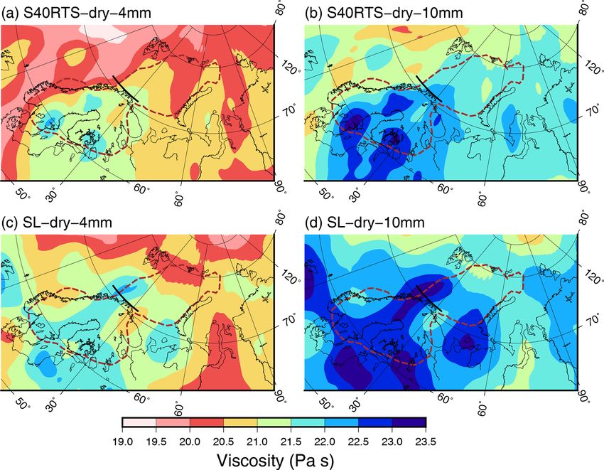
380              M. Rovira-Navarro et al.: GRACE constraints on Earth rheology of the Barents Sea and Fennoscandia

the last decade, more geological and glaciological observa-            The rheology of the Barents Sea region is expected to be
tions relevant for reconstructing the SBKIS have been ob-           different from that of Fennoscandia, as it borders passive
tained and compiled in the first version of the DATabase of         oceanic margins in the north and the west. Seismic tomogra-
Eurasian Deglaciation (DATED-1), resulting in new ice sheet         phy reveals lower seismic velocities in Barents Sea than be-
limits for the whole Eurasian Ice Sheet Complex (EISC)              low Fennoscandia (Levshin et al., 2007; Schaeffer and Lebe-
(Hughes et al., 2016), but ice thickness variations cannot be       dev, 2013) but not for all seismic periods and depths. 3D
uniquely established.                                               viscosity profiles have been implemented in GIA models for
   Comparing the GRACE-derived gravity disturbance rates            the regions and have been found to affect sea level and up-
with those predicted for different paleo-ice sheet configu-         lift rates (Kaufmann and Wu, 1998). However, the difference
rations, Root et al. (2015a) conclude that the SBKIS con-           in properties between Fennoscandia and Barents Sea has not
tained less ice than previously thought. Kachuck and Cathles        been studied explicitly.
(2018) use GRACE data, along with relative sea level (RSL)             Constraints from palaeoshoreline data on 1D GIA mod-
curves and GPS uplift measurements, to distinguish between          els resulted in best-fitting upper mantle viscosities of 2–6 ×
two deglaciation histories: one with an ice sheet with a cen-       1020 Pa s in the Barents Sea region (Steffen and Kaufmann,
tral dome in the Barents Sea and one with the Barents Sea           2005), while recent work based on RSL data finds that the
marginally glaciated and domes in the surrounding Arctic is-        best-fitting upper mantle viscosity in the Barents Sea region
lands. They show that the data are inconclusive in this regard.     is above 2 × 10²⁰ Pa s (Auriac et al., 2016). For Fennoscan-
   Since the gravity disturbance rate signal in the Barents Sea     dia, the best-fitting upper mantle viscosity is found to be
region is small, it is important to thoroughly analyze the un-      between 3 and 7 × 10²⁰ Pa s based on RSL data and relax-
certainty in GRACE data. Here we present an extended anal-          ation time spectra, while best-fitting models based on GPS
ysis of GRACE data in the region and the different uncer-           uplift rate measurements have upper mantle viscosities up to
tainty sources. We focus on the gravity disturbance rate due        15 × 1020 Pa s; see the overview in Steffen and Wu (2011).
to non-tidal mass variations in the ocean, which influence the      More recent work summarized in Simon et al. (2018) shows
secular signal from GRACE data in oceanic areas (de Linage          an upper mantle viscosity in the range of 3.4–20 × 1020 Pa s.
et al., 2009). In the processing chain to obtain Level 2            Note that the lower bound for upper mantle viscosity in the
GRACE data, changes in ocean-bottom pressure are removed            Barents Sea is somewhat below that in Fennoscandia. Steffen
using the Ocean Model for Circulation and Tides (OMCT)              and Kaufmann (2005) computed RSL misfit and find similar
forced with atmospheric data from the European Centre for           upper mantle viscosity for the Barents Sea and the Scandina-
Medium-Range Weather Forecasts (ECMWF). However, the                vian mainland but smaller lower mantle viscosity. However,
OMCT secular signal is not reliable and should not be inter-        the different studies used different ice histories and relied on
preted geophysically (Dobslaw et al., 2013). Lemoine et al.         multiple data sources, with substantially less coverage in the
(2007) used a different ocean model in their GRACE data             Barents Sea region. Therefore it is unknown if it can be con-
processing and found significant differences in the southern        cluded from previous 1D studies whether viscosity is indeed
Arctic ocean.                                                       lower in the Barents Sea than in Fennoscandia.
   We compare GRACE-derived gravity disturbance rates                  In this study we analyze GRACE data in the Barents Sea
to GIA model output to constrain the input of the GIA               region and Fennoscandia in order to obtain the GIA signal
model. Because of uncertainty in solid Earth parameters and         there, focusing on the first region where the signal-to-noise
deglaciation history, it is difficult to uniquely constrain both.   ratio is lower. We compare the estimated signal with 1D GIA
However, we can compare the GIA models for the Bar-                 model output to infer upper or lower bounds in viscosity for
ents and Kara Sea areas with models for Fennoscandia con-           different ice deglaciation chronologies. From comparison be-
strained by the same data. In this way we can determine if          tween the best-fitting models for the two regions we draw
there is a difference in Earth properties for both regions that     conclusions on the variation in Earth rheology between the
is systematic for all deglaciation chronologies. Such con-          Barents Sea and Fennoscandia.
straints on variation in viscosity are useful for GIA model-
ing and geodynamic modeling in general, as viscosity maps
derived from laboratory experiments and seismic velocities          2     Methodology
are not sufficiently constrained (e.g., Barnhoorn et al., 2011).
Furthermore, the Barents Sea is located on a continental mar-       2.1    GRACE data processing
gin, and knowledge of the subsurface rheology can help de-
cipher its tectonic history. Our aim is to provide a constraint     Temporal variations in the Earth’s gravity field measured by
on upper mantle viscosity for the Barents Sea region and            GRACE are related to mass transport within the Earth sys-
Fennoscandia, focusing on the difference in viscosity be-           tem due to different geophysical processes, such as hydrol-
tween the two regions. We build on existing knowledge of            ogy, ongoing cryospheric mass changes, GIA and (post-)
Earth rheology and ice histories, which will be briefly re-         seismic signals (e.g., Wouters et al., 2014). To study GIA,
viewed in the following.                                            other geophysical signals that mask the GIA signal should

Solid Earth, 11, 379–395, 2020                                                                www.solid-earth.net/11/379/2020/
M. Rovira-Navarro et al.: GRACE constraints on Earth rheology of the Barents Sea and Fennoscandia                                381

be removed. Additionally, GRACE data are affected by in-            wavelength signals while retaining most of the SBKIS GIA
strumental noise and the anisotropic sampling of the signal         signal (see Root et al., 2015a, Supporting Information). As
due to the orbit of the satellites (Wahr, 2007; Flechtner et al.,   the signal in Fennoscandia is larger and has a larger wave-
2016). Different data-processing techniques have been devel-        length we only use the low-pass filter there with a half width
oped to increase the GRACE signal-to-noise ratio (e.g., Han         that also ranges from 200 to 300 km.
et al., 2005; Swenson and Wahr, 2006; Kusche et al., 2009).            The total observed gravity signal (Fig. 1a, b, d) cannot
In the following, we detail the postprocessing used to ana-         be directly interpreted as the GIA footprint of the paleo-ice
lyze GRACE data in the Barents Sea and Fennoscandia, with           sheet as it contains the trend of other geophysical processes
a focus on the Barents Sea as it presents additional difficul-      as well, one of them being hydrology. Secular changes in
ties due to the smaller magnitude of the signal.                    land water storage result in gravity trends that should be sub-
    In our analysis we use the University of Texas Center           tracted when analyzing GRACE data in continental areas.
for Space Research (UTCSR) release 5 (RL05) (Bettadpur,             The long-term hydrology signal in Fennoscandia is probably
2012) up to spherical harmonic degree 60. The difference            small, as demonstrated by the good agreement between GIA
between GRACE solutions up to degree 96 and degree 60               signals derived from GRACE and GPS (van der Wal et al.,
is shown to mainly manifest as north–south oriented stripes         2011). However, the hydrology signal of the Russian Arctic
characteristic of the high-frequency noise in GRACE, with           archipelago (Novaya Zemlya, Franz Josef Land and Sever-
a magnitude at the noise level (Sakumura, 2014); therefore          naya Zemlya) can leak into oceanic areas. We subtract the
we do not use the coefficients beyond degree 60. Further-           hydrology signal using the GLDAS hydrology model (Rodell
more, their influence would be reduced because of the fil-          et al., 2004). Because its reliability for the islands of the Rus-
tering that is applied in our processing as explained later         sian Arctic archipelago is not well known, we follow Matsuo
in this section. We use data for the 2003–2015 period. We           and Heki (2013) and take the amplitude of its trend in the
substitute the degree 2 coefficients with those obtained from       Barents Sea as an indication of the uncertainty in the hydrol-
satellite laser ranging (Cheng et al., 2013). We use the least-     ogy signal in these polar regions (σhydrology ).
squares method to obtain the secular, annual and semiannual            Present-day changes in the cryosphere and the resulting
signals of each time series of Stokes coefficients. We esti-        present-day solid Earth response can also mask the GIA sig-
mate GRACE measurement errors (σGRACE ) using the resid-            nal. In particular, the glaciers of the islands of Svalbard and
uals after the secular, annual and semiannual signals are re-       the Russian Arctic archipelago are experiencing significant
moved from the signal (Wahr et al., 2006).                          mass changes evident in GRACE observations, which partly
    After processing the signal as explained above, the GIA         mask the GIA signal in the Barents Sea region (see Fig. 1).
signal is evident as a positive gravity rate in Fennoscandia        Independent data on mass changes in Svalbard and the Rus-
and the Barents Sea (Fig. 1a). However, the signal is contam-       sian Arctic archipelago are limited. Moholdt et al. (2012)
inated by the correlated noise in the higher-degree GRACE           derived trends using ICESat for the 2003–2009 period us-
data; this is evident as north–south oriented stripes. We use a     ing altimetry; other authors (e.g., Schrama et al., 2014; Mat-
Gaussian filter to filter out short-wavelength noise and apply      suo and Heki, 2013) have used GRACE data. For the period
the same filters and maximum spherical harmonic degree to           2003–2008, GRACE estimates are lower than altimetry esti-
the GIA model output. The choice for filter half width affects      mates but agree within uncertainty (Root et al., 2015a). In Si-
the signal-to-noise ratio. Earlier studies in Scandinavia used      mon et al. (2018) ice mass loss estimates from altimetry and
a 400 km half width Gaussian filter (e.g., Steffen and Denker,      glaciology for a longer period were shown to be much larger
2008; van der Wal et al., 2011), but the better accuracy of         than GRACE estimates in Svalbard, Franz Josef Land and
later GRACE data releases and longer time series since then         Novaya Zemlya, and altimetry estimates were scaled down
allow less filtering. To account for the fact that the optimum      in that study. Here we follow Root et al. (2015a) and use
filter half width is not known, we adopt a range of high-pass       ice loss corrections obtained using the mascon method of
filter half widths from 200 to 300 km. At 200 km half width         Schrama et al. (2014) (see Table 1) to remove the ice loss
correlated noise (stripes) are still visible (Fig. 1a, b), while    signal taking into account elastic loading (Wahr et al., 1998).
for filter half widths larger than 300 km the positive gravity         To obtain the present-day mass changes from GRACE, a
anomaly in the Barents Sea is very small (Fig. 2). Low-pass         GIA correction needs to be first applied As our aim is to
filtering to reduce the measurement noise inevitably means          quantify the GIA signal in the central Barents Sea, the prob-
that some sensitivity to possible high-frequency signal con-        lem seems circular. However, the GIA model has a relatively
tent in the GIA models is lost; that is, we cannot assess de-       small effect on the derived present-day mass changes. We ac-
tailed changes in ice thickness based on our GRACE gravity          count for uncertainty in mass loss estimations due to GIA by
rates. We additionally use a high-pass filter in the Barents        employing an ensemble of ice deglaciation chronologies and
Sea to remove the long-wavelength signal that contains long-        Earth rheological parameters. We use the ICE-5G model and
wavelength phenomena such as global sea level rise that are         two runs of the GSM ice model (Tarasov et al., 2012) with
not modeled. The high-pass filter half width ranges from 500        maximum and minimum ice sheet extents combined with the
to 700 km, which was found to be optimal to remove long-            VM5a Earth model (Peltier, 2004) and an Earth model with a

www.solid-earth.net/11/379/2020/                                                                  Solid Earth, 11, 379–395, 2020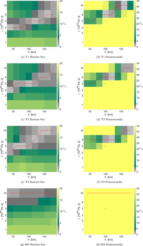
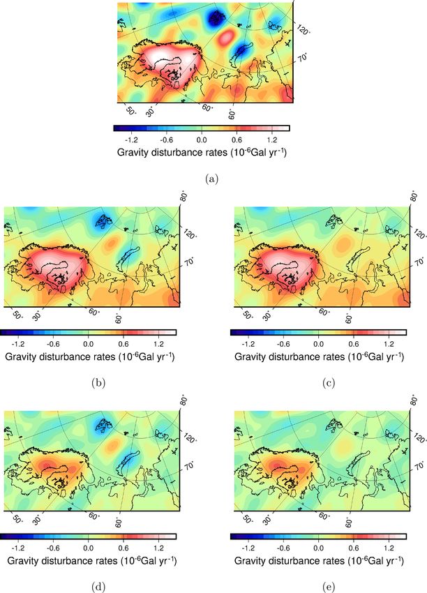
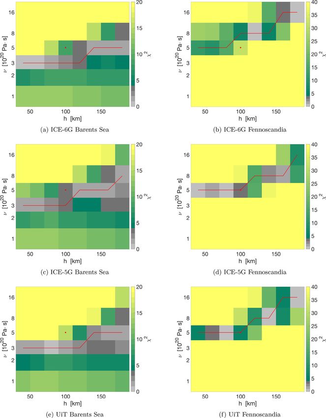
382               M. Rovira-Navarro et al.: GRACE constraints on Earth rheology of the Barents Sea and Fennoscandia

Figure 1. Gravity signal in Fennoscandia and the Barents Sea for the period 2003–2015. Panel (a) shows the gravity disturbance trends for
the unprocessed GRACE data. Panels (b) and (c) show the gravity disturbance rate filtered with a 200 km low-pass filter, while in (d) and
(e) the data are additionally filtered with a 600 km high-pass filter to remove long-wavelength signals. The mass loss signal of the Russian
Arctic archipelago islands has been removed in (c) and (e).

stronger mantle, as well as the W12 ice model (Whitehouse               due to uncertainty in GIA is similar to the GRACE mea-
et al., 2012) with a strong mantle. Mass loss changes ob-               surement error. We use the error bars of the estimated mass
tained using the different GIA models are shown in Table 1;             changes for Svalbard and the Russian Arctic archipelago to
more massive ice sheet models and stronger mantles result in            estimate the error in the recovered GIA gravity rates due to
higher mass loss rates. The error in the derived mass changes           uncertainty in mass loss changes in the region (σice ). Finally,

Solid Earth, 11, 379–395, 2020                                                                      www.solid-earth.net/11/379/2020/
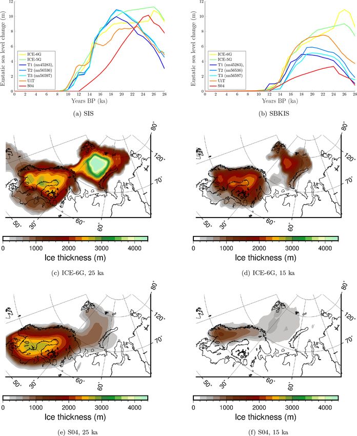
M. Rovira-Navarro et al.: GRACE constraints on Earth rheology of the Barents Sea and Fennoscandia                                       383

Figure 2. Volume of ice present in the (a) SIS and (b) SBKIS during the last glacial period, given in equivalent eustatic sea level rise for
different ice sheet reconstructions. Six different deglaciation chronologies are shown, including the following: the GIA-constrained models
ICE-5G and ICE-6G (Peltier, 2004; Peltier et al., 2015; Argus et al., 2014); three models obtained using the Glacial System Model (GSM)
(Tarasov et al., 2012), the T1, T2 and T3 chronologies; the University of Tromsø Ice Sheet Model (UiT) (Patton et al., 2017); and the S04 ice
sheet model (Siegert and Dowdeswell, 2004). The divide between both ice sheets is taken to be the 70◦ parallel. Ice extent and thickness are
shown for the (c, d) ICE-6G and (e, f) S04 ice models for two different epochs.

for the Barents Sea, the Greenland mass loss is already fil-             ucts (monthly non-tidal oceanic mass anomalies simulated
tered when using the high-pass filter, but for Fennoscandia              by the OMCT ocean model) to restore the full GRACE ocean
we need to remove it. To do so we use ICESat mass changes                mass signal (Flechtner et al., 2015; Yu et al., 2018) before
from Sørensen et al. (2011).                                             subtracting the ECCO ocean model. The ECCO model is
   We account for the uncertainty in non-tidal ocean changes             a dynamically consistent ocean model constrained with ob-
by using the ECCO ocean model (Forget et al., 2015) as al-               servations from altimetry, Argo floats and GRACE. The
ternative for the ocean model used in standard GRACE level               model has been shown to correctly capture long-term bot-
2 processing. In that case we first add back the GAB prod-               tom pressure variability in the Arctic Ocean and adjacent

www.solid-earth.net/11/379/2020/                                                                        Solid Earth, 11, 379–395, 2020
384              M. Rovira-Navarro et al.: GRACE constraints on Earth rheology of the Barents Sea and Fennoscandia

Table 1. Ice loss changes in Svalbard and the islands of the Russian Arctic archipelago between 2003 and 2015 in Gt yr−1 , obtained for
different GIA models. The ICE-5G model and two runs of the GSM with maximum (GLAC2) and minimum (GLAC1) ice sheet extents,
which comply with RSL and GPS observations combined with the VM5 Earth rheological model or a model with stronger mantle, labeled
M2, with µUM = 1.6×10²¹ Pa s and µLM = 5.12×10²² Pa s. Additionally, the W12 ice model with µUM = 1×10²¹ Pa s and µLM = 1×10²²
(M3) is also used. The last row indicates the average value and uncertainty due to GRACE measurement error and uncertainty in the GIA
model.

                     Ice model   Rheology     Novaya Zemlya          Svalbard    Franz J. Land   Severnaya Zemlya
                     GLAC1       M2               4.71 ± 0.42      5.05 ± 0.49    1.12 ± 0.19         0.76 ± 0.10
                     GLAC1       VM5a             4.94 ± 0.42      4.96 ± 0.49    1.10 ± 0.19         0.63 ± 0.10
                     GLAC2       M2               4.60 ± 0.42      4.90 ± 0.49    0.93 ± 0.19         0.92 ± 0.10
                     GLAC2       VM5a             4.57 ± 0.42      4.85 ± 0.49    0.85 ± 0.19         0.67 ± 0.10
                     ICE-5G      M2               5.87 ± 0.42      5.77 ± 0.49    1.68 ± 0.19         0.80 ± 0.10
                     ICE-5G      VM5a             4.54 ± 0.42      5.16 ± 0.49    1.03 ± 0.19         0.70 ± 0.10
                     W12         M3               6.13 ± 0.42      5.34 ± 0.49    1.64 ± 0.19         0.46 ± 0.10
                     –           –                5.15 ± 0.58      5.05 ± 0.79    1.19 ± 0.38         0.70 ± 0.18

seas (Peralta-Ferriz, 2012). The version of the ocean model            2.2   GIA Modeling
we use is the ECCOv4-llc270 compilation. This compilation
covers the period 2001–2015, which means the GRACE time
series that we use in the Barents Sea is limited to this period.       We compare GRACE-derived gravity rates with those pre-
We obtain gravity rates in the central Barents Sea using the           dicted by GIA models. To compute the gravity trends the
UTCSR GRACE solution corrected with both the OMCT and                  sea level equation is solved, using the pseudo-spectral ap-
the ECCO ocean models. The differences between these two               proach presented in Mitrovica and Peltier (1991). We use
solutions are used as an indication of the uncertainty in non-         the same code as Barletta and Bordoni (2013). To be able
tidal ocean changes (σocean ).                                         to run calculations for many different Earth parameters and
   We estimate the total error in the gravity trends by assum-         ice models we assume that solid Earth properties only vary
ing that the different error sources are uncorrelated as fol-          radially, which allows us to compute GIA response for dif-
lows:                                                                  ferent regions separately with different viscosity profiles
                                                                       but neglects effects of viscosity changes in surrounding re-
     q
σ = σice 2 +σ2             2        2                        (1)
               GRACE + σocean + σhydrology .                           gions. While this approach has been used in other GIA stud-
                                                                       ies (Lambeck et al., 1998; Steffen et al., 2014), it has been
The assumption that errors are uncorrelated requires further
                                                                       suggested that far-field viscosity variations are relevant in
discussion. GRACE data are assimilated in the ECCO ocean
                                                                       Fennoscandia (Whitehouse et al., 2006).
model. However, GRACE is only one of the 40 data sets
                                                                          We neglect the loading effect due to sediment transport
used in the inversion process, and the final product does not
                                                                       during deglaciation, as the effect is small and well below
fit GRACE data well (Yu et al., 2018). Therefore there will
                                                                       that of the unknown ice thickness (0.01 to 0.05 µGal yr−1
be only a weak correlation with the GRACE data used in
                                                                       in Fennoscandia and below 0.014 µGal yr−1 in the Barents
our estimation. Correlation between land surface hydrology
                                                                       Sea, as shown in van der Wal and Ijpelaar, 2017). To study
models and present-day ice melt is not expected, because hy-
                                                                       the effect of the ice deglaciation history on the present grav-
drology models have little skill in predicting trends and do
                                                                       ity rates we start by using a reference Earth model based
not model areas of permanent snow. Finally, ice loss change
                                                                       on the averaged VM2 model, which is similar to the VM5a
errors (σice ) arise due to uncertainty in the GIA model and
                                                                       model (Peltier, 2004; Argus et al., 2014). The model con-
GRACE measurement error; we cannot rule out that the sec-
                                                                       sists of a 90 km lithosphere, a 570 km upper mantle with a
ond error component might be correlated with σGRACE .
                                                                       viscosity of 0.5 × 10²¹ Pa s and a 2216 km lower mantle with
    For the Barents Sea we consider the four terms, while for
                                                                       an average viscosity of 2.6 × 10²¹ Pa s. The elastic proper-
Fennoscandia we only consider GRACE measurement er-
                                                                       ties of the Earth are based on the PREM model (Dziewonski
rors, as the ice loss changes in the Russian Arctic archipelago
                                                                       and Anderson, 1981). To investigate the effect of the Earth’s
and ocean-bottom pressure changes have a very small effect
                                                                       rheology, we vary the upper mantle viscosity between 0.1
on the gravity trends recovered in Fennoscandia, and Green-
                                                                       and 1.6 × 10²¹ Pa s and the lithospheric thickness between
land’s mass loss signal is well known from altimetry mea-
                                                                       40 and 180 km (Table 2). We do not change the lower man-
surements.
                                                                       tle as its viscosity cannot be constrained uniquely from data
                                                                       in Fennoscandia (Steffen and Kaufmann, 2005). However,
                                                                       gravity rates are influenced by the lower mantle viscosity,

Solid Earth, 11, 379–395, 2020                                                                   www.solid-earth.net/11/379/2020/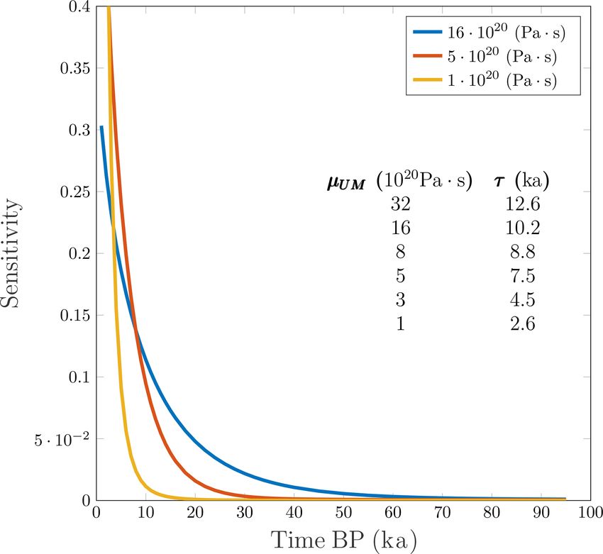
M. Rovira-Navarro et al.: GRACE constraints on Earth rheology of the Barents Sea and Fennoscandia                                 385

Table 2. Solid Earth rheological parameters for this study: litho-       The University of Tromsø Ice Sheet Model is based on a
sphere thickness (hl ), upper mantle viscosity νUM and lower mantle   3D thermomechanical ice model which uses an approxima-
viscosity νLM .                                                       tion of the Stokes equations forced by climatic and eustatic
                                                                      sea level perturbations to simulate the evolution of the EISC.
          Parameter          Reference model      Range               The model is constrained using different geophysical and
          hl (km)                           90   40–180               geological data sets including geomorphological flow sets,
          νUM (1021 Pa s)                  0.5   0.1–1.6              moraine and grounding zone wedge positions, and isostasy
          νLM (1021 Pa s)                  2.6       2.6              patterns and is consistent with the DATED-1 ice sheet mar-
                                                                      gins. Isostatic loading is implemented using the elastic litho-
                                                                      sphere/relaxed asthenosphere model of Le Meur and Huy-
                                                                      brechts (1996). The model has no ice in the region before
which is discussed in the comparison with other GIA studies           37 ka.
for the region.                                                          Finally, we consider an ice sheet model which gives a
   We use an ensemble of ice histories that reflects the uncer-       lower bound for the mass present in the Barents Sea during
tainty in the deglaciation history of the European Ice Sheet          the LGM, the S04 model (Siegert and Dowdeswell, 2004).
Complex (EISC), the amount of ice in the SBKIS and the                The model is based on the continuity flow equations coupled
Scandinavian Ice Sheet (SIS) for the different ice deglacia-          with a model of water, basal sediment deformation and trans-
tion scenarios shown in Fig. 2 . The ice sheet models that we         portation. The model is forced with eustatic sea level curves
use can be divided into two main categories: (1) empirical            of the last 30 ka, paleo-air temperatures and precipitation and
ice sheet models based on GIA observables and empirically             assumes an ice-free scenario before 32 ka. Bedrock topogra-
determined ice extents and (2) those based on numerical ice-          phy is adjusted for isostasy using the method of Oerlemans
sheet modeling forced under different paleo-climate scenar-           and van der Veen (1984).
ios and tuned to fit different constrains. A fundamental dif-            The only global ice sheet models are the ICE-5G and
ference between these two kinds of models is that GIA-based           ICE-6G; for the other ice sheet models we use the ICE-6G
paleo-ice sheet models are explicitly associated with a spe-          ice model outside the EISC. We include the build-up and
cific Earth model. The first set of models is represented by          deglaciation phase of the last glacial cycle. All ice sheet mod-
the ICE-5G and ICE-6G models (Peltier, 2004; Peltier et al.,          els are sampled in a grid with a spatial resolution correspond-
2015; Argus et al., 2014). Both models start the ice build-up         ing to a 128◦ Gaussian grid, and the output of the model is
at 122 ka. The second set consists of three models obtained           truncated at degree 60 and processed using the same filters
using the Glacial System Model (GSM) for northern Europe              used to process the GRACE data.
(Tarasov et al., 2012), the University of Tromsø Ice Sheet
Model (UiT ISM) (Patton et al., 2016, 2017) and the S04 ice           2.3    Model performance assessment
sheet model (Siegert and Dowdeswell, 2004), which are fur-
ther described below. Figure 2 shows the ice model with the           We assess the fit of the modeled and estimated gravity rates
largest LGM ice volume (ICE-6G) and the model with the                for different combinations of ice deglaciation history and
smallest ice volume (S04).                                            rheology. As GRACE’s resolution is of the same order of
   The three ice sheet models obtained using the GSM model            magnitude as the extension of the SBKIS we cannot resolve
are a subset of a bigger ensemble used in Root et al. (2015a),        the differences in the shape of the ice sheet in the data. Thus
which showed good agreement with GRACE observations.                  we assess the model fit only by comparing the maximum
The ensemble was obtained using a Bayesian calibration                modeled (mi ) and estimated (ei ) gravity rate in the central
of GSM runs with RSL curves, present-day ground veloci-               Barents Sea and Fennoscandia and normalize this difference
ties and ice deglaciation margins from the DATED-1 project            using the observation error (σi ). In order to make the results
(Hughes et al., 2016). The VM5a rheology model was em-                as independent of the filter parameters as possible, we com-
ployed as reference during the calibration process; however,          pute an average misfit using different filter configurations as
errors introduced by the rheology model were accounted                follows:
for during the calibration process, which implies that this                     N
                                                                                    ei − mi 2

model is not as strongly biased by a single viscosity pro-                   1 X
                                                                      χ2 =                    ,                                   (2)
file as the ICE-5G and ICE-6G models. The three selected                     N i=1     σi
models consist of a late deglaciation model, labeled nn45283
in Root et al. (2015a) and two early deglaciation models,             where N is the number of filter settings. The low-pass filter
nn56536 and nn56597, with different maximum ice volumes.              is varied between 200 and 300 km half width in 20 km in-
The build-up phase is faster than for the ICE-5G and ICE-6G           tervals. Additionally, in the Barents Sea the high-pass filter
models; build-up starts 28 ka. The models will be labeled T1          is varied between the 500 and 700 km half width in 100 km
(nn45283), T2 (nn56536) and T3 (nn56597) to simplify the              intervals. We cannot formally define a confidence region as
notation.                                                             GRACE’s observations, which are processed with different

www.solid-earth.net/11/379/2020/                                                                   Solid Earth, 11, 379–395, 2020
386 M. Rovira-Navarro et al.: GRACE constraints on Earth rheology of the Barents Sea and Fennoscandia
filter configurations, do not form a set uncorrelated observa-
tions. Instead, we define a subset of best-fitting models as
those that differ less than 2σ from the observations, indicat-
ing that, given the measurement noise, any of these models
could be the best-fitting model for a different realization of
the observations. In the following we will refer to the lowest
upper mantle viscosity of this set as lower bound.
3 Results
3.1 GRACE GIA signal in Fennoscandia and the
Barents Sea
We use the methods presented in Sect. 2 to obtain the gravity
rates over Fennoscandia and the Barents Sea. A clear posi- Figure 3. Maximum gravity rate in µGal yr−1 recovered in the cen-
tive anomaly is evident both in Fennoscandia and the central tral Barents Sea using GRACE, after removing the ocean signal with
Barents Sea where the main domes of the Scandinavian Ice the OMCT ocean model (blue) or ECCO ocean model (orange) for
Sheet and Svalbard–Barents–Kara Ice Sheet were presum- different low-pass filter half widths and a 600 km half width high-
ably located (Fig. 1). The melting of ice in Svalbard and the pass filter. The GIA signal for different ice deglaciation histories
islands of the Russian Arctic archipelago is also evident as with the reference Earth model is also shown.
a negative gravity trend. After removing the mass loss sig-
nal as explained in Sect. 2, we observe that most of the sig-
nal of Novaya Zemlya, Svalbard and Franz Josef Land is 3.2 Implications for viscosity and ice sheet chronology
indeed removed (Fig. 1). However, there is still a negative
gravity rate left over Severnaya Zemlya, indicating that our We perform three experiments. In the first experiment we
ice loss changes might be underestimated for this island. We only study the effect of the ice history on the model misfit.
consider the remaining part of the signal to be entirely due We use the reference Earth model (see Table 2) and compare
to GIA and call it the estimated GIA signal. We do not ob- the fit of the predicted gravity rates for different ice deglacia-
serve a clear positive signal in the Kara Sea, which indicates tion models with the GRACE-derived gravity rate. In the sec-
that if it was glaciated during the LGM, the amount of ice ond experiment, we change the Earth rheological parameters
present there was much smaller than that located in the Bar- to obtain the subset of ice deglaciation histories and Earth
ents Sea. This fact advocates against the larger ice sheets rheological parameters that best fit the GRACE observations.
in Denton and Hughes (1981); Grosswald (1998); Gross- Thirdly, we repeat the second experiment for Fennoscandia
wald and Hughes (2002) and further confirms the results of and compare the optimal solid Earth parameters for both re-
the DATED-1 (Hughes et al., 2016) and QUEEN projects gions to detect possible variations in rheological parameters.
(Svendsen et al., 2004). Figure 3 compares the maximum present-day estimated
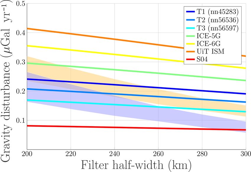
We obtain the maximum gravity rate in the Barents Sea for gravity rates in the Barents Sea with those given by the dif-
different filter configurations using the OMCT and ECCO ferent ice sheet models. It must be noted that the maximum
ocean models. Figure 3 shows the maximum gravity rates gravity rates produced by each ice history are related to not
for a 600 km high-pass filter and different low-pass filter half only the maximum ice volume attained during LGM, but also
widths. As expected, we observe that the maximum gravity its geographical distribution and the onset of the deglaciation
signal reduces with increasing filter half width and so does process. As an example, we find that while the T2 model has
the error. The gravity rates recovered using the ECCO ocean more ice in the Barents Sea than the T1 model, it results in
model are systematically higher that those obtained with the lower gravity rates. This is because deglaciation starts earlier
OMCT model. We show a breakdown of the error (Fig. 4) for in the T2 model than in the T1 model, when the sensitivity of
different low-pass filter half widths. We observe that the hy- the present gravity rates to mass changes is higher as shown
drology signal leaking into the Barents Sea is very small and in Fig. 5. Similarly, the highest gravity rates are associated
the error budget is dominated by the uncertainty in present- with the UiT ISM even though it has less ice than the ICE-5G
day ice changes, the GRACE measurement error and the non- and ICE-6G models. This is because the UiT ice sheet model
tidal ocean signal. Moreover, we observe that while the other has more ice in the central Barents Sea during the last phase
error sources decrease with increasing filter half width, the of deglaciation. In fact, the model includes an ice bridge be-
ocean error does not. This implies that it has a wavelength tween Svalbard, Franz Josef Land and Novaya Zemlya with
similar to that of the GIA signal we want to resolve. ice thickness as large as 2000 m at 14.5 ka which does not
disappear until 12 ka. This is not present in either the ICE-
6G or the ICE-5G models.
Solid Earth, 11, 379–395, 2020 www.solid-earth.net/11/379/2020/M. Rovira-Navarro et al.: GRACE constraints on Earth rheology of the Barents Sea and Fennoscandia 387
Figure 4. Error in µGal yr−1 in the maximum gravity rate in the central Barents Sea from different sources. The magnitude of the error is
given for different low-pass filter half widths and a high-pass filter half width of 600 km.
GRACE-derived estimations is reduced if we use the ECCO
ocean model instead of the OMCT. Furthermore, GRACE
data can be reconciled with the UiT ISM if the maximum
volume of mass in the model is reduced by around 1 m of
equivalent sea level rise or if deglaciation started 1 kyr earlier.
Next, we study the effects of changing the solid Earth rhe-
ology in the Barents Sea. Figures 6a, c, e and g and 7a, c and
e show the misfit of the different ice sheet models to the esti-
mated maximum gravity rates in the Barents Sea for different
rheology models. We see that there is a large subset of Earth
rheological parameters for which the modeled gravity rate is
within 2σ of GRACE’s estimated gravity rate.
The T1, T2 and T3 ice sheet models present a good fit
to the observations for a large subset of Earth models includ-
ing the reference Earth model (ν = 5×10²⁰ Pa s; h = 90 km).
For the less massive S04 model the 2σ interval extends from
ν = 8 × 10²⁰ to ν = 1.6 × 10²¹ Pa s. In contrast, for the more
massive ice sheets (ICE-5G, ICE-6G and UiT ISM) the sub-
set of Earth models which present a good fit to the Barents
Figure 5. Present gravity disturbance rate induced by a uniform Sea observations is smaller and does not contain the refer-
mass change in the Barents Sea at a given epoch for three differ- ence Earth model. These models, however, fit the observa-
ent upper mantle viscosity. The results have been normalized us- tions for either a less viscous upper mantle or a thicker litho-
ing the maximum gravity disturbance rate obtained with µUM = sphere when upper mantle viscosity is fixed. If a less vis-
1 × 10²⁰ Pa s. Inset: relaxation times for different upper mantle vis- cous upper mantle viscosity is used, the relaxation time of the
cosity. solid Earth is decreased, and the sensitivity to mass changes
that occurred during the LGM decreases (see Fig. 5). On
the other hand, a thicker lithosphere acts as a low-pass fil-
When we compare the modeled and estimated gravity rates
ter, which smooths the gravity signal, reducing its maximum
we find that, for the reference Earth model, the T1, T2 and
value.
T3 ice sheet models are the closest to observations. The S04
Our results for the UiT ISM are consistent with those
ice sheet model performs worse; the model does not have
obtained by Patton et al. (2017), which inferred an upper
enough ice in the region. This result is in accordance with
mantle viscosity of 2 × 10²⁰ Pa s based on RSL data. The
Auriac et al. (2016), which found poor agreement between
lower bound obtained with the other ice models is similar
the S04 model and RSL curves. The more massive ICE-5G,
as models with a low viscosity have little sensitivity to mass
ICE-6G and UiT models result in gravity rates that are too
changes during the early deglaciation phase, where differ-
high. However, the discrepancy between these models and
www.solid-earth.net/11/379/2020/ Solid Earth, 11, 379–395, 2020388 M. Rovira-Navarro et al.: GRACE constraints on Earth rheology of the Barents Sea and Fennoscandia Figure 6. Misfit of the T1, T2, T3 and S04 ice deglaciation chronologies to GRACE observations for different values of upper mantle viscosity (ν) and lithospheric thickness (h) in (a, c, e, g) the Barents Sea and (b, d, f, h) Fennoscandia. The fit is given in terms of the χ 2 . The circle indicates the reference model, and the red line shows the best-fitting model for each lithospheric thickness. Solid Earth, 11, 379–395, 2020 www.solid-earth.net/11/379/2020/
M. Rovira-Navarro et al.: GRACE constraints on Earth rheology of the Barents Sea and Fennoscandia                              389

Figure 7. Same as Fig. 6 but for the ICE-6G, ICE-5G and UiT ice sheet models.

ences between ice models are more manifest (Fig. 2). Over-              We follow the same procedure for Fennoscandia to ob-
all, for a lower mantle viscosity of 2.6 × 10²¹ Pa s, we obtain      tain the subset of Earth rheological parameters and ice sheet
a lower bound for the upper mantle viscosity of 3×10²⁰ Pa s,         deglaciation histories with an acceptable agreement with the
which agrees with the range of possible upper mantle viscos-         GRACE observations (see Figs. 6b, d, f and h and 7b, d and
ity found in Auriac et al. (2016) using RSL curves and GPS           f). It must be noted that the values of the χ 2 are higher for
uplift measurements. We refrain from drawing conclusions             Fennoscandia than the Barents Sea, and thus the subset of
on the preferred lithosphere thickness from the misfit plots         models within the 2σ contour is smaller. The reason is 2-fold:
because the lithosphere has a large influence on the shape           the observation error is smaller as compared with the Barents
of the gravity rate pattern, which was not used as constraint        Sea, where uncertainty from mass changes in the glaciers of
here. A higher lower mantle viscosity can result in a lower          the surrounding islands and non-tidal ocean changes increase
upper mantle viscosity that still provides a good fit, as shown      the error bars; and the GIA signal is higher in Fennoscan-
in Steffen et al. (2010), Root et al. (2015b).                       dia than in the Barents Sea (see Fig. 1). Nevertheless we can
                                                                     compare the best-fitting models for both regions.

www.solid-earth.net/11/379/2020/                                                                 Solid Earth, 11, 379–395, 2020
390 M. Rovira-Navarro et al.: GRACE constraints on Earth rheology of the Barents Sea and Fennoscandia
We observe that, contrary to what we got for the Bar- lations from geochemistry (Goes et al., 2000; Cammarano
ents Sea, the combination of the ice sheet models ICE-5G et al., 2003) for primitive mantle composition and accounting
and UiT with the reference lithospheric thickness and up- for anelasticity (anelastic correction model Q4 from Cam-
per mantle viscosity have a good fit (Figs. 6 and 7). As al- marano et al., 2003). Differences in composition between the
ready mentioned, the ICE-5G and ICE-6G models have been Barents Sea and Scandinavia could play a role but is unlikely
constrained using GIA observations, which are abundant in to reverse the temperature contrast, due to the first order ef-
Fennoscandia. As we are using these models with an Earth fect of temperature on seismic velocities in the upper mantle
rheology similar to its reference rheology it is not surprising (Goes et al., 2000). To compute viscosity we follow the pro-
that the ICE-5G model presents a good fit in this region; how- cedure in Wal et al. (2013) and insert temperatures in the
ever the ICE-6G model performs better with a more viscous olivine flow laws of Hirth and Kohlstedt (2013). The flow
mantle due to its lower ice volume. The T1–3 models do not laws for diffusion and dislocation are added, which means
fit the estimated GIA signal with the reference Earth model the viscosity depends on grain size and stress. Stress is taken
and require a more viscous mantle. The early deglaciation from a 3D GIA model which uses the ICE-5G ice load. Back-
and small LGM ice volume of the S04 model results in low ground stresses due to mantle convection are neglected as re-
gravity disturbance rates that do not fit the GRACE estimated cent work suggest little interaction between GIA and mantle
gravity disturbance rates for the set of rheology parameters convection (Huang, 2018). Grain size is chosen to be 4 or
considered in this study. For Fennoscandia we find a lower 10 mm. The 4 mm size gave best overall fit to GIA data, and
bound for the upper mantle viscosity of 5 × 10²⁰ Pa s, which 10 mm grain size resulted in the best fit with the observed
is consistent with current estimates (Simon et al., 2018). maximum uplift rate (Wal et al., 2013).
We can infer lateral rheology changes by comparing the To be able to compare against viscosity for the upper man-
optimal Earth rheological parameters obtained for both re- tle in the previous section we use viscosity averaged between
gions. For each ice deglaciation chronology, we compare the 225 and 325 km. This depth is a trade-off; shallower lay-
two 2σ intervals as well as the best-fitting upper-mantle vis- ers have lower temperature and small viscous deformation
cosity obtained for each lithospheric thickness. We observe during the glacial cycle, while for deeper layers the seismic
that for the UiT, ICE-5G and ICE-6G models both the 2σ models are less accurate. The depth range is also close to
intervals and the best-fitting models systematically prefer a the depth to which the gravity rate in Fennoscandia is most
less viscous upper mantle in the Barents Sea as compared sensitive; see the sensitivity kernels in van der Wal et al.
with Fennoscandia. This is also the case for the T1,T2 and T3 (2011). The viscosity maps are plotted in Fig. 8. In princi-
models when the best-fitting models are compared, although ple all viscosity values around the ice load play a role in the
there is an overlap of models of high upper mantle viscosity GIA process, but the highest sensitivity is to values directly
and thick lithospheres with a good fit in both regions. This underneath the ice load (Paulson et al., 2005; Wu, 2006). We
systematic difference is likely evidence of lateral variation in compute the average of viscosities for the locations where
Earth rheology. LGM ice heights are above 1500 m, which covers most of the
land mass of Scandinavia and most of the Barents Sea (see
3.3 Lateral viscosity variation dashed brown contour). Viscosity is computed separately for
the region below 71◦ latitude for Fennoscandia and above
To strengthen the conclusion of viscosity differences be- for the Barents Sea. We find that the average viscosity below
tween the two regions, we derive viscosity estimates in an in- Fennoscandia is a factor of 2.3 to 2.4 times higher than that
dependent way, based on seismic velocity anomalies and ex- in the Barents Sea. This agrees well with the change in best
perimentally derived flow laws. The absolute viscosity values fit upper mantle viscosity that can be seen in the misfit Figs. 6
obtained in this way contain large uncertainty, but the relative and 7. There could still be an effect of 3D structure that is not
difference resulting from the seismic models should repre- captured by modeling both regions with 1D models, such as
sent real change in temperature or composition. Therefore we lateral variations within Fennoscandia (Steffen et al., 2014)
focus on the ratio between the viscosities beneath Fennoscan- or the influence of viscosity from outside each region.
dia and the Barents Sea and check whether it agrees with the
outcome of the GIA model misfit.
To take uncertainty in seismic velocity anomalies into 4 Conclusions and discussion
account we use two global seismic tomography models:
S40RTS (Ritsema et al., 2011) and Schaeffer and Lebe- In this study, we analyze GRACE data in the Barents Sea to
dev (2013) (labeled SL), which has higher spatial resolu- constrain the Earth rheology in the region. We compare the
tion but reduced sensitivity with depth. For both, the refer- fit of different GIA models in Fennoscandia with that for the
ence model is adjusted to account for a jump in the seis- Barents Sea to find if there is a difference in viscosity be-
mic velocity anomaly in PREM (Dziewonski and Ander- tween the two regions. We investigate several deglaciation
son, 1981) and AK135 (Kennett et al., 1995) below 200 km. chronologies of the SBKIS, some of which are not explicitly
Shear wave velocities are converted to temperature using re- tied to a viscosity model. We use GRACE data for the period
Solid Earth, 11, 379–395, 2020 www.solid-earth.net/11/379/2020/M. Rovira-Navarro et al.: GRACE constraints on Earth rheology of the Barents Sea and Fennoscandia 391 Figure 8. Viscosity between depths of 225 and 325 km derived from seismic models (a, b) S40RTS (Ritsema et al., 2011) and (c, d) Schaeffer and Lebedev (2013) and for different flow law parameters: (a, c) 4 mm grain size and (b, d) 10 mm grain size. The brown line denotes the 1500 m ice height contour at LGM in the ICE-5G model; the black line denotes 71◦ latitude, which separates the areas used for computing the viscosity for Fennoscandia and the Barents Sea. 2003–2015 and process the data to reveal the GIA signal. We compare the GRACE-derived gravity rates with mod- The ice loss signal from the Svalbard and the Russian Arctic eled ones to infer geophysical constraints for the Earth rheol- archipelago is removed using mass change values obtained ogy and ice sheet chronology in the Barents Sea region. For from GRACE using the mascon method. We observe a pos- a three-layer average of the VM2 viscosity profile (Peltier, itive gravity anomaly in the Barents Sea but no significant 2004) we find, as Root et al. (2015a), that thick ice sheet anomaly in the Kara Sea, which shows that the ice cover at models (ICE-5G, ICE-6G and UiT) do not fit GRACE obser- LGM was considerably thinner there than in the Barents Sea, vations, while the less massive ice models (T1,T2 and T3) in agreement with recent studies. do. Upper mantle viscosity and lithospheric thickness were The Barents Sea GIA signal is in a region now covered by varied for each ice sheet chronology between 0.1 × 10²¹ and sea; therefore, the gravity trends might be affected by non- 1.6 × 10²¹ Pa s and 40 and 180 km. We find that the ICE-5G, tidal oceanic mass changes. We correct GRACE gravity rates ICE-6G and UiT ice sheet models can be reconciled with in the Barents Sea using either of the two ocean models, GRACE observations provided the upper mantle viscosity is OMCT and ECCO, and find higher gravity rates using the lower or the lithosphere thicker than in the VM2 model. The ECCO model. The difference in the ocean signal according same conclusion is reached in Auriac et al. (2016) using GPS to the two models is large in the Barents Sea. This uncer- uplift measurements and RSL curves instead of gravity data. tainty has not been considered in previous studies of the GIA The interplay between ice deglaciation chronology and signal in the region (e.g., Root et al., 2015a; Simon et al., Earth rheology makes it difficult to constrain the ice deglacia- 2018; Kachuck and Cathles, 2018), and thus the errors bars tion chronology in the Barents Sea (Kachuck and Cathles, in those studies were underestimated. This result has also im- 2018). Root et al. (2015a) used GRACE data to conclude plications for GRACE studies of non-oceanic mass changes, that the SBKIS had less ice than previously thought (5–6.3 m such as post seismic deformations, in ocean areas (e.g., Han of equivalent sea level versus 8.3 m). To do so, they used and Simons, 2008; Wang et al., 2012), which possibly have ICE-5G and ICE-6G and showed that they do not obtain higher uncertainty than previously thought due to errors in the estimated gravity rate when these ice models are com- the ocean model. bined with their corresponding Earth rheology model. How- www.solid-earth.net/11/379/2020/ Solid Earth, 11, 379–395, 2020
392                M. Rovira-Navarro et al.: GRACE constraints on Earth rheology of the Barents Sea and Fennoscandia

ever, here we use the UiT ISM, which does not come with                 Competing interests. The authors declare that they have no conflict
an a priori Earth rheology model and contains around 7.5 m              of interest.
of equivalent sea level rise and show that the model can fit
GRACE observations provided the upper mantle viscosity is
around 3×10²⁰ Pa s if the lithosphere is thinner than 130 km.           Acknowledgements. The authors would like to thank Lev Tarasov,
However, we are able to place a constraint on upper mantle              Henry Patton and Martin J. Siegert for making their ice sheet models
viscosity. From the misfit of all investigated ice chronologies         available for this study (T1, T2 and T3; UiT ISM and S05 model).
                                                                        The authors also thank Ernst J. O. Schrama for providing mass loss
and using a lower mantle viscosity of 2.6 × 10²¹ Pa s, we find
                                                                        changes in the islands of the Russian Arctic archipelago for this
that best-fitting models have an upper mantle viscosity equal
                                                                        work and Ward Stolk for his contribution to the viscosity maps. The
to or higher than 3 × 10²⁰ Pa s, which agrees with previous             authors also thank Ian Fenty for his assistance and advice on the
constraints derived from RSL and GPS uplift observations                ECCO ocean model products. Marc Rovira-Navarro would like to
Auriac et al. (2016).                                                   thank Fundacio la Caixa for the financial support he received while
   We also study the misfit of GRACE observations to the                conducting this research.
GIA models in Fennoscandia. For a 2.6 × 10²¹ Pa s lower
mantle viscosity, best-fitting models have an upper man-
tle viscosity equal to or higher than 5 × 10²⁰ Pa s, which is           Financial support. This research has been partially supported by
consistent with current estimates. Given all of the ice sheet           La Caixa Foundation postgraduate studies program.
deglaciation chronologies we find that the lower bound for
the upper mantle viscosity is a factor of 2 smaller in the Bar-
ents Sea (or, alternatively, the lithosphere thickness should           Review statement. This paper was edited by Nicolas Gillet and re-
be increased there). Unless all of the tested ice deglaciation          viewed by two anonymous referees.
chronologies are biased in the same direction, this result is
evidence of lateral changes in viscosity in between the two
regions.                                                                References
   To strengthen the finding of viscosity difference between
the two regions, we compare our results with viscosity de-              Argus, D. F., Peltier, W. R., Drummond, R., and Moore, A. W.: The
                                                                          Antactica component of postglacial rebound model ICE-6G_C
rived from global velocity anomalies and flow laws for man-
                                                                          (VM5a) based on GPS positioning, exposure age dating of ice
tle material and find that the average viscosity in the Bar-
                                                                          thickness and relative sea level histories, Geophys. J. Int., 198,
ents Sea is a factor of 2.4 lower than in Fennoscandia. This              537–563, https://doi.org/10.1093/gji/ggu140, 2014.
agrees very well with the results derived from the misfit of            Auriac, A., Whitehouse, P. L., Bentley, M. J., Patton, H.,
GIA models to GRACE data and strengthens the conclusion                   Lloyd, J. M., and Hubbard, A.: Glacial isostatic adjust-
that there is a small but significant difference in average up-           ment associated with the Barents Sea ice sheet : A mod-
per mantle viscosity between the two regions. This findings               elling inter-comparison, Quaternary Sci. Rev., 147, 122–135,
have implications for ice sheet models inverted with just one             https://doi.org/10.1016/j.quascirev.2016.02.011, 2016.
viscosity profile (e.g., ICE-5G, ICE-6G) and advocates in fa-           Barletta, V. and Bordoni, A.: Effect of different implementations of
vor of including lateral Earth rheological parameters in GIA              the same ice history in GIA modeling, J. Geodyn., 71, 65–73,
models. The constraints on viscosity variations can be also               https://doi.org/10.1016/j.jog.2013.07.002, 2013.
                                                                        Barnhoorn, A., van der Wal, W., and Drury, M. R.: Upper mantle
used to calibrate other geodynamic models of the regions.
                                                                          viscosity and lithospheric thickness under Iceland, J. Geodyn.,
                                                                          52, 260–270, https://doi.org/10.1016/j.jog.2011.01.002, 2011.
                                                                        Bettadpur, S.: Gravity Recovery and Climate Experiment Level-2
Code and data availability. Gravity rates for the different ice sheet     Gravity Field Product User Handbook, UTCSR, Texas, USA,
models and Earth rheology models and GRACE maximum dis-                   2012.
turbance rates for Fennoscandia and the Barents Sea are pro-            Cammarano, F., Goes, S., Vacher, P., and Giardini, D.: Infer-
vided at https://doi.org/10.4121/uuid:424126e6-b5d3-4ac9-b5cd-            ring upper-mantle temperatures from seismic velocities, Phys.
f495c8ad6939 (Rovira-Navarro et al., 2019). The GIA code used             Earth Planet. Int., 138, 197–222, https://doi.org/10.1016/S0031-
for the simulations is available upon request from Valentina R. Bar-      9201(03)00156-0, 2003.
letta.                                                                  Cheng, M., Tapley, B. D., and Ries, J. C.: Deceleration in the
                                                                          Earth’s oblateness, J. Geophys. Res.-Sol. Ea., 118, 740–747,
                                                                          https://doi.org/10.1002/jgrb.50058, 2013.
Author contributions. All authors contributed to the discussion and     de Linage, C., Rivera, L., Hinderer, J., Boy, J.-P., Rogister, Y.,
commented on the manuscript. MRN and WvdW led the writing                 Lambotte, S., and Biancale, R.: Separation of coseismic and
of the article. VRB contributed with her GIA code. MRN analyzed           postseismic gravity changes for the 2004 Sumatra-Andaman
GRACE data and ran the GIA simulations. WvdW provided the 3D              earthquake from 4.6 yr of GRACE observations and mod-
viscosity maps. All authors contributed to the interpretation of the      elling of the coseismic change by normal-modes summation,
results.                                                                  Geophys. J. Int., 176, 695–714, https://doi.org/10.1111/j.1365-
                                                                          246X.2008.04025.x, 2009.

Solid Earth, 11, 379–395, 2020                                                                      www.solid-earth.net/11/379/2020/
M. Rovira-Navarro et al.: GRACE constraints on Earth rheology of the Barents Sea and Fennoscandia 393 Denton, G. and Hughes, T.: The Last Great Ice Sheets, Wiley- Kachuck, S. B. and Cathles, L. M.: Constraining the geometry and Interscience, New York, 1981. volume of the Barents Sea Ice Sheet, J. Quaternary Sci., 33, 527– Dobslaw, H., Flechtner, F., Dahle, C., Dill, R., Esselborn, S., Sas- 535, https://doi.org/10.1002/jqs.3031, 2018. gen, I., and Thomas, M.: Simulating high-frequency atmosphere- Kaufmann, G. and Wu, P.: Lateral asthenospheric viscos- ocean mass variability for dealiasing of satellite gravity obser- ity variations and postglacial rebound: A case study for vations : AOD1B RL05, J. Geophys. Res., 118, 3704–3711, the Barents Sea, Geophys. Res. Lett., 25, 1963–1966, https://doi.org/10.1002/jgrc.20271, 2013. https://doi.org/10.1029/98GL51505, 1998. Dziewonski, A. M. and Anderson, D. L.: Preliminary refer- Kennett, B. L. N., Engdahl, E. R., and Buland, R.: Con- ence Earth model, Phys.e Earth Planet. Int., 25, 297–356, straints on seismic velocities in the Earth from traveltimes, https://doi.org/10.1016/0031-9201(81)90046-7, 1981. Geophys. J. Int., 122, 108–124, https://doi.org/10.1111/j.1365- Flechtner, F., Dobslaw, H., and Fagiolini, E.: AOD1B Product De- 246X.1995.tb03540.x, 1995. scription Document for Product Release 05, GFZ German Re- Kusche, J., Schmidt, R., Rietbroek, S., and Petrovic, R.: Decorre- search Centre for Geosciences, Potsdam, Germany, 2015. lated GRACE time-variable gravity solutions by GFZ , and their Flechtner, F., Neumayer, K.-H., Dahle, C., Dobslaw, H., Fagi- validation using a hydrological model, J. Geodesy, 83, 903–913, olini, E., Raimondo, J.-C., and Güntner, A.: What Can be https://doi.org/10.1007/s00190-009-0308-3, 2009. Expected from the GRACE-FO Laser Ranging Interferometer Lambeck, K.: Constraints on the Late Weichselian ice sheet for Earth Science Applications?, Surv. Geophys., 37, 453–470, over the Barents Sea from observations of raised shorelines, https://doi.org/10.1007/s10712-015-9338-y, 2016. Quaternary Sci. Rev., 14, 1–16, https://doi.org/10.1016/0277- Forget, G., Campin, J.-M., Heimbach, P., Hill, C. N., Ponte, R. M., 3791(94)00107-M, 1995. and Wunsch, C.: ECCO version 4: an integrated framework for Lambeck, K., Smither, C., and Johnston, P.: Sea-level change, non-linear inverse modeling and global ocean state estimation, glacial rebound and mantle viscosity for northern Europe, Geosci. Model Dev., 8, 3071–3104, https://doi.org/10.5194/gmd- Geophys. J. Int., 134, 102–144, https://doi.org/10.1046/j.1365- 8-3071-2015, 2015. 246x.1998.00541.x, 1998. Goes, S., Govers, R., and Vacher, P.: Shallow mantle tem- Le Meur, E. and Huybrechts, P.: A comparisonon if different ways peratures under Europe from P and S wave tomog- of dealing with isostasy: Examples from modelling the Antarctic raphy, J. Geophys. Res.-Sol. Ea., 105, 11153–11169, ice sheet during the last grlacial cycle, Ann. Glaciol., 23, 309– https://doi.org/10.1029/1999JB900300, 2000. 317, 1996. Grosswald, M. G.: Late Weichselian ice sheet of Northern Eura- Lemoine, J.-M., Bruinsma, S., Loyer, S., Biancale, R., Marty, J.- sia, Quaternary Res., 13, 1–32, https://doi.org/10.1016/0033- C., Perosanz, F., and Balmino, G.: Temporal gravity field models 5894(80)90080-0, 1980. inferred from GRACE data, Adv. Space Res., 39, 1620–1629, Grosswald, M. G.: Late-Weichselian ice sheets in Arc- https://doi.org/10.1016/j.asr.2007.03.062, 2007. tic and Pacific Siberia, Quaternary Int., 45, 3–18, Levshin, A. L., Schweitzer, J., Weidle, C., Shapiro, N. M., and https://doi.org/10.1016/S1040-6182(97)00002-5, 1998. Ritzwoller, M. H.: Surface wave tomography of the Barents Grosswald, M. G. and Hughes, T. J.: The Russian component of Sea and surrounding regions, Geophys. J. Int., 170, 441–459, an Arctic Ice Sheet during the Last Glacial Maximum, Qua- https://doi.org/10.1111/j.1365-246X.2006.03285.x, 2007. ternary Sci. Rev., 21, 121–146, https://doi.org/10.1016/S0277- Mangerud, J., Astakhov, V., and Svendsen, J.-I.: The extent of the 3791(01)00078-6, 2002. Barents Kara ice sheet during the Last Glacial Maximum, Qua- Han, S.-C. and Simons, F. J.: Spatiospectral localization of global ternary Sci. Rev., 21, 111–119, https://doi.org/10.1016/S0277- geopotential fields from the Gravity Recovery and Climate Ex- 3791(01)00088-9, 2002. periment (GRACE) reveals the coseismic gravity change owing Matsuo, K. and Heki, K.: Current Ice Loss in Small Glacier to the 2004 Sumatra-Andaman earthquake, J. Geophys. Res.-Sol. Systems of the Arctic Islands (Iceland, Svalbard, and Ea., 113, B01405, https://doi.org/10.1029/2007JB004927, 2008. the Russian High Arctic) from Satellite Gravimetry, Han, S.-C., Shum, C. K., Jekeli, C., Kuo, C.-Y., Wilson, C., and Terrestial Atmospheric Oceanic Science, 24, 657–670, Seo, K.-W.: Non-isotropic filtering of GRACE temporal gravity https://doi.org/10.3319/TAO.2013.02.22.01(TibXS), 2013. for geophysical signal enhancement, Geophys. J. Int., 163, 18– Mitrovica, J. X. and Peltier, W. R.: On postglacial geoid subsidence 25, https://doi.org/10.1111/j.1365-246X.2005.02756.x, 2005. over the equatorial oceans, J. Geophys. Res.-Sol. Ea., 96, 20053– Hirth, G. and Kohlstedt, D.: Rheology of the upper mantle and 20071, https://doi.org/10.1029/91JB01284, 1991. the mantle wedge: A view from the experimentalists, in: Inside Moholdt, G., Wouters, B., and Gardner, A. S.: Recent mass changes the Subduction Factory, 2004, edited by: Eiler, J., Geophysical of glaciers in the Russian High Arctic, Geophys. Res. Let., 39, Monograph Series, American Geophysical Union (AGU), Black- l10502, https://doi.org/10.1029/2012GL051466, 2012. well Publishing Ltd, 83–105, https://doi.org/10.1029/138GM06, Oerlemans, J. and van der Veen, C. J.: Bedrock Ad- 2013. justment, Springer Netherlands, Dordrecht, 111–123, Huang, P.: Modelling Glacial Isostatic Adjustment with Composite https://doi.org/10.1007/978-94-009-6325-2_7, 1984. Rheology, PhD thesis, The University of Hong Kong, Pokfulam, Patton, H., Hubbard, A., Andreassen, K., Winsborrow, M., and Hong Kong, 2018. Stroeven, A. P.: The build-up , configuration , and dynamical Hughes, A. L. C., Gyllencreutz, R., Lohne, O. Y. S., Mangerud, sensitivity of the Eurasian ice-sheet complex to Late Weichselian J., and Inge, J.: The last Eurasian ice sheets – a chronological climatic and oceanic forcing, Quaternary Sci. Rev., 153, 97–121, database and time-slice reconstruction, DATED-1, Boreas, 45, https://doi.org/10.1016/j.quascirev.2016.10.009, 2016. 1–45, https://doi.org/10.1111/bor.12142, 2016. www.solid-earth.net/11/379/2020/ Solid Earth, 11, 379–395, 2020
You can also read