Skilful prediction of cod stocks in the North and Barents Sea a decade in advance
←
→
Page content transcription
If your browser does not render page correctly, please read the page content below
ARTICLE
                  https://doi.org/10.1038/s43247-021-00207-6              OPEN

                  Skilful prediction of cod stocks in the North and
                  Barents Sea a decade in advance
                  Vimal Koul 1,2 ✉, Camilla Sguotti3, Marius Årthun4, Sebastian Brune2, André Düsterhus                                      5,   Bjarte Bogstad6,
                  Geir Ottersen6,7, Johanna Baehr2 & Corinna Schrum1,2

                  Reliable information about the future state of the ocean and fish stocks is necessary for
                  informed decision-making by fisheries scientists, managers and the industry. However,
                  decadal regional ocean climate and fish stock predictions have until now had low forecast
                  skill. Here, we provide skilful forecasts of the biomass of cod stocks in the North and Barents
1234567890():,;

                  Seas a decade in advance. We develop a unified dynamical-statistical prediction system
                  wherein statistical models link future stock biomass to dynamical predictions of sea surface
                  temperature, while also considering different fishing mortalities. Our retrospective forecasts
                  provide estimates of past performance of our models and they suggest differences in the
                  source of prediction skill between the two cod stocks. We forecast the continuation of
                  unfavorable oceanic conditions for the North Sea cod in the coming decade, which would
                  inhibit its recovery at present fishing levels, and a decrease in Northeast Arctic cod stock
                  compared to the recent high levels.

                  1 Helmholtz Zentrum Hereon, Institute of Coastal Systems, Geesthacht, Germany. 2 Institute of Oceanography, Center for Earth System Research and

                  Sustainability, Universität Hamburg, Hamburg, Germany. 3 Institute for Marine Ecosystem and Fisheries Science, Center for Earth System Research and
                  Sustainability, Universität Hamburg, Hamburg, Germany. 4 Geophysical Institute, University of Bergen and Bjerknes Centre for Climate Research,
                  Bergen, Norway. 5 Irish Climate Analysis and Research UnitS (ICARUS), Department of Geography, Maynooth University, Maynooth, Ireland. 6 Institute of
                  Marine Research, Bergen, Norway. 7 Centre for Ecological and Evolutionary Synthesis, Department of Biosciences, University of Oslo, Oslo, Norway.
                  ✉email: vimal.koul@uni-hamburg.de

                  COMMUNICATIONS EARTH & ENVIRONMENT | (2021)2:140 | https://doi.org/10.1038/s43247-021-00207-6 | www.nature.com/commsenv                            1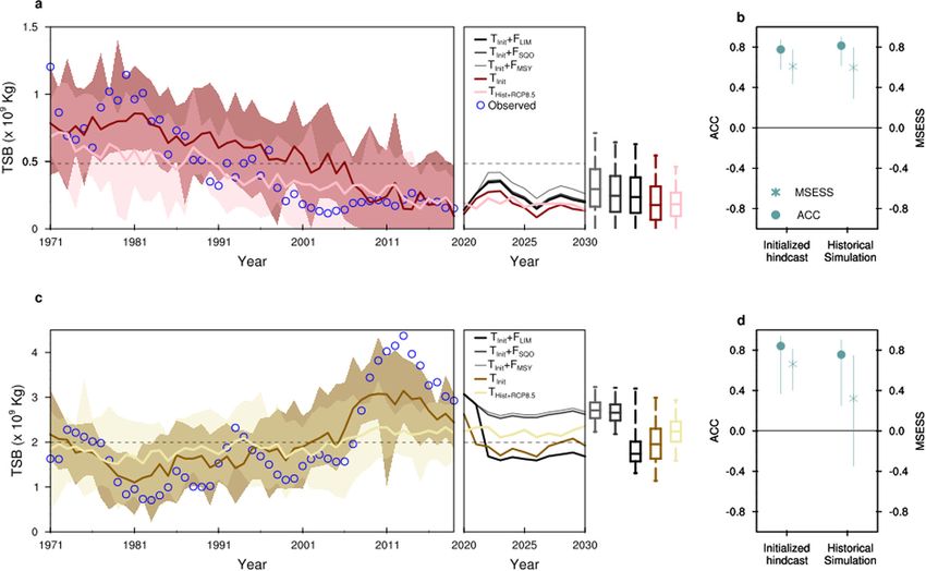
ARTICLE                                             COMMUNICATIONS EARTH & ENVIRONMENT | https://doi.org/10.1038/s43247-021-00207-6

C
        limate variability has been a subject of interest for ecolo-       of the North Atlantic shelf seas, such as the North and Barents
        gists primarily because variations in climate often have a         Sea15,16 but also from the impact of anthropogenic warming on
        strong impact on ecological systems1. Marine resources,            marine ecosystems13. In these climate-driven marine ecosystems,
such as fish stocks, have been shown to be strongly influenced by            statistical climate–fisheries models36 provide a promising
climate variability2–4, with changes in productivity resulting in          approach for transforming GCM-based ensembles of decadal
huge consequences for socio-economic systems relying on such               climate predictions into reliable fisheries forecasts.
resources5,6. In the Anthropocene, with the impending threat of               In this article we assess predictability of two Atlantic cod
climate change, understanding the impact of climate variability            (Gadus morhua) stocks in the northeastern North Atlantic shelf
on marine ecosystems and resources has become even more                    seas. Atlantic cod is a commercially, historically, socially, and
central, since climate variability at interannual to decadal time-         ecologically important species. There are many stocks of Atlantic
scales can alter the magnitude of ongoing long-term climate                cod and they are widely distributed on the shelf seas off the
change7,8. Hence an integration of climate information into                northern North Atlantic. Some of these stocks have been severely
modeling of exploitable resources is necessary not only to                 reduced in the last decades, largely due to unfavorable climate
understand ecological processes but also to forecast future states         and intense fishing20,22. Thus, being able to predict the
of the system at interannual to decadal timescales9. The latter is         stock biomasses is important to guide sustainable management
particularly fundamental for management, since forecasting fish             decisions. We investigate two stocks with opposite status: (1)
abundance depending on decadal climate variability is necessary            the North Sea cod, a stock close to the upper temperature limit
to devise timely interventions to ensure sustainable use of                of distribution of this species, over-exploited for many decades
resources10. Nevertheless, the application of climate models to            and in a very low productive state over the last 20 years, and
predict ecosystem processes at decadal timescales remains a                (2) the Northeast Arctic cod, residing in the Barents Sea
challenge11–13.                                                            close to the species’ lower temperature limit and recording
   In many cases the impact of climate on fish stocks has been              record-high biomass levels in recent years37–39. The average age
studied through experiments and modeling, and empirical rela-              at first maturation is 3 for North Sea cod and 7 for Northeast
tions have been established. Climate has been shown to influence            Arctic cod.
fish directly or indirectly through recruitment, food availability,            In order to provide decadal predictions of cod stocks, we use a
fecundity, growth, and migration14–16. Still, climate variables            linear regression model to transform dynamical prediction of sea
are rarely included in the management-oriented modeling and                surface temperature (SST) into the prediction of total stock bio-
forecasting of fish populations17. This is not only due to his-             mass (TSB). TSB was used because it reflects the integrated
torically large impact of fishing mortality on commercial stock             impact of climate and fishing36. The dynamical prediction of SST
biomass18–20 but also due to forecasting being complicated by              is provided by 10-year long initialized forecasts (and hindcasts)
frequent transient and non-stationary properties of climate                from a decadal prediction system based on the Max Planck
impacts on fish stocks21–23. Moreover, the fish experience the               Institute Earth System Model (MPI-ESM, see “Methods”). The
cumulative impacts of different drivers; fishing pressure and cli-          initial conditions for decadal hindcasts are taken from an
mate can have combined effects inducing non-linear dynamics in             assimilation experiment which assimilates observed atmospheric
fish stocks. Strong synergistic effects can lead to management              and oceanic information into MPI-ESM. In order to isolate the
failures and abrupt collapses of socio-ecological systems22,24,25.         prediction skill due to external forcing, an ensemble of non-
With anthropogenic climate change superposed on natural cli-               initialized historical simulations of the same size as that of
mate variability, including environmental variables in the mod-            initialized hindcasts and driven by observed external boundary
eling and forecasting of fish stocks is becoming increasingly               conditions is also analyzed (see “Methods”). Our forecasts for the
important from both scientific and management points of                     period 2020–2030 suggest continued unfavorable environmental
view5,26.                                                                  conditions for the North Sea cod with no significant recovery
   One of the key limitations impeding the integration of climate          under any of the three different fishing mortality scenarios. For
information in fisheries forecasts originates from inadequate               the Northeast Arctic cod, assuming fishing at the current sus-
representation of shelf seas in coupled global circulation models          tainable level is continued, we forecast a decline in TSB in the
(GCMs) providing future climate information. Pioneering-                   coming decade compared to the last decade, attributed mainly to
approaches have used bioclimate envelope models27,28 or detailed           a decline in temperature.
ecosystem and population dynamics models29,30 forced with cli-
mate projections from GCMs to examine the impact of climate
change on fisheries. However, GCMs lack a proper representation             Results
of shelf-sea dynamics, mainly due to their coarse resolution, and          Variability in cod stocks and their physical environment. The
they have limited representation of trophic interactions and asso-         time series of SST in the North Sea and Barents Sea Opening
ciated energy transfers. Other approaches have combined GCM                highlight key differences in the two regions: While SST has an
output with highly resolved physical–biological shelf-sea models           increasing trend both in the North Sea and in the Barents Sea
accounting for trophic interactions6. These approaches focus on            Opening, the absolute values are very different from each other,
long-term (>30 years) changes and thus do not provide information          highlighting that the cod stocks reside at the two extreme ends of
on decadal (1–10 years) fisheries forecasts. Moreover, since decadal        the thermal habitat available for cod40 (Fig. 1a). The TSB time
forecasting usually involves an ensemble of predictions, high              series of the two stocks also show opposite development: North
computational costs associated with the aforementioned approaches          Sea cod has declined continuously since the 1960s, with very low
also motivate exploration of novel approaches towards fisheries             and stable biomass levels since the beginning of the twenty-first
predictions using GCM-based decadal climate predictions.                   century (Fig. 1b). Northeast Arctic cod exhibits multi-annual to
   The prospect of decadal prediction of fish stocks emerging               decadal variability for the same period, with a recent record high
from decadal predictability of the physical environment is enti-           level of TSB (Fig. 1b). However, multi-decadal variability in
cing. Specifically in the North Atlantic, where decadal variability         North Sea stock biomass has been reported for a longer period41.
of the physical environment is highly predictable using                    Fishing mortality (F) trends are similar in these two stocks,
GCMs31–33. This prospect emerges not only from the influence of             increasing in the central period of the time series and recently
Atlantic inflow on both hydrography34,35 and marine ecosystem               declining as stricter management measures started to be enforced

2           COMMUNICATIONS EARTH & ENVIRONMENT | (2021)2:140 | https://doi.org/10.1038/s43247-021-00207-6 | www.nature.com/commsenv
COMMUNICATIONS EARTH & ENVIRONMENT | https://doi.org/10.1038/s43247-021-00207-6                                                            ARTICLE

Fig. 1 Observed variability in temperature and cod stocks. a Time series of annual mean sea surface temperature from observations and the assimilation
experiment (see “Methods”) for the North Sea (NOR, red lines), subpolar gyre (SPG, orange lines), and the Barents Sea Opening (BSO, purple lines).
b Time series of total stock biomass (TSB, green and blue circles) and fishing mortality (F, green and blue lines) for the cod stocks in the North and Barents
Sea. The inset in a shows regions over which the temperature is averaged (boxes) and the ICES ecoregions (color-filled) for delimiting cod stocks.

(Fig. 1b). Interestingly, while the decline in fishing mortality of              work36. Dynamically, this linkage points to the influence of SPG
Northeast Arctic cod seems to have resulted in an increase in                   circulation on the properties of Atlantic water crossing the
TSB, in the North Sea, the cod stock did not manage to recover                  Greenland–Scotland ridge heading towards downstream shelf
even after the management measures were in place. This has been                 seas34,35,42.
attributed to the effect of an interacting driver (i.e. warming)                   After removing respective trends from time series of the SPG
which has inhibited the productivity of North Sea cod22.                        temperature and Northeast Arctic cod TSB, the correlation
   In the North Sea SST, the magnitude of warming over the                      remains high (r = 0.77, p = 0.0425), suggesting a dominating
period 1960–2019 (1.68 °C) is more than twice the year-to-year                  signature of decadal variability. The effect of temperature is
variability (σ = 0.65 °C), indicating that the increasing tempera-              opposite on this stock compared to the North Sea, since in the
ture trend is part of how the North Sea has changed under natural               Barents Sea, temperature has a positive impact on cod biomass.
and anthropogenic forcing, and thus the trend cannot be                         These opposite impacts of temperature on biomass reflect the
excluded from the analysis. Temperature increase corresponds                    different temperature regimes in which the stocks reside22,43. In
to decrease in TSB, thus there is a negative correlation between                the case of Northeast Arctic cod, fishing mortality of 5–10-year-
the two variables. Linearly detrended North Sea temperature                     old cod is strongly correlated with TSB (r = −0.88, p = 0.00351).
maintains the same negative effect on TSB the following year (r                 This correlation is higher than the one between temperature and
= −0.48, p = 0.0025, see Supplementary Figs. S1 and S2 for                      TSB, and peaks at lag-2 years (Supplementary Fig. 2). For our
detailed statistical analysis). Interestingly, the fishing mortality of          purpose of decadal prediction of cod biomass this finding has two
2–4-year-old cod does not exhibit a monotonous trend and does                   implications. First, the predictability horizon for TSB from a
not show a strong correlation with TSB (r = −0.19, p > 0.05). This              statistical point of view would be shorter with fishing mortality as
weak signal might partly be due to the fact that a decline in                   a predictor compared to temperature. Second, the higher
fishing mortality in the last years did not correspond to an                     explanatory power in fishing mortality might constrain the
increase in TSB (Fig. 1b). The low correlation exhibited by fishing              uncertainty in the first few years of forecasts.
mortality may limit its usage as a predictor for TSB using linear
models and could indicate a time-varying F–TSB relationship
typical of systems presenting discontinuous dynamics.                           Statistical models for cod prediction. Once the predictors for the
   The TSB of Northeast Arctic cod does not exhibit a long-term                 two cod stocks are identified, we assess various cross-validated
trend (Fig. 1b). This stock exhibits multi-annual to decadal                    statistical models (see “Methods”) to analyze the retrospective
variability manifested as multiple cycles of decline and increase.              skill arising from the impact of temperature and fishing on the
Similar low-frequency variability is visible in the surface                     TSB and to select a model to issue forecasts. We test three dif-
temperature of the North Atlantic subpolar gyre (SPG),                          ferent models, two simple linear regression models based on
suggesting a possible linkage. Statistically, this linkage is                   temperature and fishing mortality separately and one multiple
supported by the high correlation between the surface tempera-                  linear regression model based on temperature and fishing mor-
ture of the SPG and TSB of Northeast Arctic cod (r = 0.78, p =                  tality as explanatory variables.
0.0435) with the SPG-temperature leading TSB by 7 years                            As expected from the correlational analysis, the results for the
(Supplementary Figs. S1 and S2), and consistent with previous                   North Sea cod and the North-East Arctic cod are quite different.

COMMUNICATIONS EARTH & ENVIRONMENT | (2021)2:140 | https://doi.org/10.1038/s43247-021-00207-6 | www.nature.com/commsenv                                    3
ARTICLE COMMUNICATIONS EARTH & ENVIRONMENT | https://doi.org/10.1038/s43247-021-00207-6
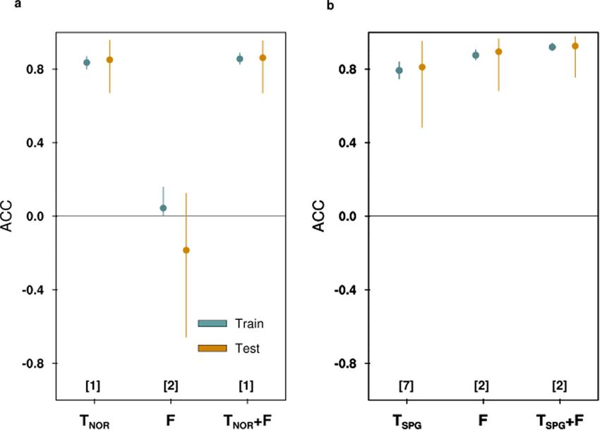
Fig. 2 Statistical models for cod prediction. a Cross-validated correlation skill from three linear regression models (two simple and one multiple) for TSB
of North Sea cod based on North Sea surface temperature (TNOR) and fishing mortality (F). b Same as (a) but for Northeast Arctic cod and using SPG
temperature (TSPG) as one of the predictors. The number in square bracket is the prediction horizon in years for each model. The dots show median skill
and the whiskers show the 95% confidence limits (see “Methods”).
For North Sea cod, the linear model using just fishing mortality forcing) in the North Sea temperature as the source of prediction
has no predictive power (Fig. 2a and Supplementary Fig. S3 for skill. Noticeable exception is the SPG where the skill is largely
analysis of skill from detrended variables). When the impacts of intact irrespective of the trend, and is higher for initialized
fishing and temperature are modeled together, the skill is hindcasts than historical simulations (Fig. 3c, d and Supple-
comparable to the linear model based on temperature alone, mentary Fig. S4).
suggesting that no additional information is gained by adding The observed and predicted time series of SPG temperature
fishing mortality. For the Northeast Arctic cod, although the suggests that during the hindcast period, most of the skill in the
fishing-only model provides a better fit to the TSB data (adjusted initialized hindcasts is derived from the ability of the model to
R2 = 0.77) than the temperature-only model (adjusted R2 = 0.62), capture the decadal cooling and warming trends (Fig. 3d). The
the difference in skill between these two models is not statistically 16-member historical simulation does not capture the full extent
significant (p = 0.15, Fig. 2b and Supplementary Fig. S3 for skill of the decadal variability in SPG temperature. Thus, it appears
from detrended variables). that initialization of oceanic conditions is the dominant source of
Out of the three models, the model which uses both predictability of SPG temperature33, while the long-term trend,
temperature and fishing has the best fit to the TSB (adjusted mainly arising from external forcing, dominates predictability in
R2 = 0.84) and is the most suited model considering the the North Sea. The robustness of the decadal prediction skill of
information gained by combining SST and F (Table S1). subpolar North Atlantic SST in the MPI-ESM-LR based decadal
However, both the fishing-only and the combined fishing and prediction systems has been thoroughly analyzed and is
temperature-based models do not allow for a longer prediction consistent with other decadal prediction systems33,44.
horizon than the temperature-only model. This is because fishing
mortality leads TSB by 2 years while temperature leads TSB by 7
years. Since our focus is on long prediction horizons, we choose Dynamical–statistical cod prediction. Now, we combine the
the temperature-only model for the hindcast period, and for the dynamical prediction of temperature with the statistical
forecast period (2020–2030), we complement the temperature- temperature–cod relationship. We choose the simplest model
based forecasts of cod biomass with forecasts from the combined with temperature as the explanatory variable for both the North
fishing and temperature-based model. Sea and Northeast Arctic cod to model and forecast TSB. The
utilization of temperature, derived from the dynamical model,
allows us to extend the predictability horizon of cod stocks. We
Decadal prediction of the physical environment. We now assess also include forecasts using a multiple linear regression model
the prediction skill of North Sea and SPG temperature in the with fishing and temperature, and we use various scenarios of
MPI-ESM (see “Methods” for a detailed description of this model fishing mortality based on current management advice from the
and the decadal prediction system). In general, the skill degrades International Council for the Exploration of the Sea (ICES).
as the prediction horizon moves farther from the year of initi- The dynamical–statistical prediction model shows robust skill
alization (i.e. at longer lead times). However, in the North Sea, (correlation as well as mean square error skill) in simulating the
prediction skill remains high until lead year-10, and is matched North Sea cod biomass (Fig. 4a). Note that the regression
by the skill from the historical simulations (Fig. 3a). This can be coefficients for the statistical models are not calculated from the
explained by the long-term linear trend in the underlying time hindcast time series of temperature, but from the observed TSB
series (Fig. 3b), which is present in all lead year time series. This and assimilated temperatures (see “Methods”). The similarity in
points to the long-term trend (driven by anthropogenic external hindcast skill obtained from initialized hindcasts and historical
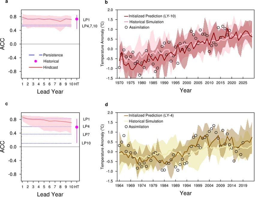
4 COMMUNICATIONS EARTH & ENVIRONMENT | (2021)2:140 | https://doi.org/10.1038/s43247-021-00207-6 | www.nature.com/commsenvCOMMUNICATIONS EARTH & ENVIRONMENT | https://doi.org/10.1038/s43247-021-00207-6 ARTICLE Fig. 3 Dynamical predictions of temperature. Anomaly correlation coefficient (ACC) as a function of lead year for initialized hindcasts (red), lagged- persistence (blue), and historical simulation (magenta dot) for annual mean (a) North Sea surface temperature and (c) subpolar gyre surface temperature with respect to the assimilation experiment for the period 1971–2019. Time series of (b) North Sea surface temperature and (d) subpolar gyre surface temperature anomalies (with respect to 1970–2019 mean) from the assimilation experiment (circles), initialized hindcast (dark colored line), forecast and historical+RCP8.5 simulation (light colored line). The solid lines in (b and d) are the respective ensemble mean predictions (or simulations) and the shading is the entire range of the respective 16-member ensemble. The regions for computing area averaged surface temperatures of the North Sea and subpolar gyre are shown in Fig. 1a. The lagged-persistence (LP)-based skill is provided for 1-, 4-, 7- and 10-year lags. The shading and whiskers in (a and c) depict 95% confidence intervals. simulations provides another piece of evidence that the skill is comparable to the skill from the historical simulation (Supple- mainly due to the trend in the North Sea temperature (Fig. 4b). mentary Fig. S4). Our dynamical–statistical prediction model Our forecast of North Sea temperature for the period performs well in reproducing past variability in the TSB of 2020–2030 suggest a continuation of the warm anomalies (Fig. 3c) Northeast Arctic cod (Fig. 4c, d). Both the 1970s decline as well as which translates into a further decline of North Sea cod (Fig. 4a). the recent decadal shift in the TSB is captured by the initialized In order to make our predictions of cod biomass usable in hindcast, quantified by the mean square error skill score (Fig. 4d). fisheries management, we provide both an SST-based forecast (for The correlation skill associated with historical simulation is lower 2020–2030) and forecasts under different fishing scenarios (using but not statistically different from the hindcast skill (p = 0.164). the SST+F model). In particular we chose three scenarios: an However, the variability in the reconstructed TSB time series of FMSY scenario, in which the biomass is fished at the maximum Northeast Arctic cod using historical simulation is suppressed sustainable yield (FMSY = 0.3), an FSQO scenario in which F is the (Fig. 4c). This reconstructed time series fails to capture the recent mean over the last three years (FSQO = 0.5), and an FLIM decadal shift in the Northeast Arctic cod stock, which, as precautionary scenario which is the maximum F applicable discussed above, likely follows variability in SPG temperature and before collapse (FLIM = 0.54). The predicted total biomass of is not captured by the historical simulation. This lack of North Sea cod shows similar trends under all these scenarios, variability in the reconstructed TSB time series using the modulated in magnitude by fishing. Lower fishing initially favors historical SPG temperature is reflected in the mean square error a stock increase, but the constant increase of temperature leads to skill score (MSESS, Fig. 4d), which suggests that this type of a further decline of the stock over time, keeping the stock in a low prediction is not significantly better than predicting a long-term productivity regime. This indicates that deteriorating environ- mean value for the TSB. mental conditions will hinder a substantial stock recovery, even For the Northeast Arctic cod, future predictions based on with strong limitation on the fishery. initialized hindcasts suggest a climate-driven decline of biomass For assessing the retrospective prediction skill of Northeast in the coming decade compared to the present stock size (Fig. 4c). Arctic cod biomass, we combine the statistical model with lead- The RCP8.5 scenario based forecast, however, suggests a biomass year-4 initialized hindcasts of SPG temperature from MPI-ESM. level close to the long-term mean. Since the historical simulation- Beyond lead-year-4, the dynamical hindcast skill degrades and is based hindcasts of cod biomass do not capture the full extent of COMMUNICATIONS EARTH & ENVIRONMENT | (2021)2:140 | https://doi.org/10.1038/s43247-021-00207-6 | www.nature.com/commsenv 5
ARTICLE                                                COMMUNICATIONS EARTH & ENVIRONMENT | https://doi.org/10.1038/s43247-021-00207-6

Fig. 4 Decadal prediction of cod stocks. a Time series of retrospective predictions of total stock biomass (TSB) of North Sea cod using the
dynamical–statistical prediction model (retrospective predictions of North Sea surface temperature combined with the linear statistical temperature–cod
relationship) for the period 1971–2019 using the initialized hindcast and historical simulation of North Sea surface temperature. The observed TSB is shown
by blue circles. Also provided is the forecast for the period 2020–2030 comprising three fishing mortality scenarios: status quo (FSQ = 0.50), maximum
sustainable yield (FMSY = 0.30), and precautionary approach (FLIM = 0.54). The bars and whiskers show the 95% confidence limits (2.5th, 25th, 50th,
75th, and 97.5th percentiles are shown) for the respective forecasts for the whole period (2020–2030). The historical North Sea surface temperature
is extended using the RCP8.5 scenario for issuing forecasts of cod biomass. b Anomaly correlation coefficient (ACC) and mean square error skill
score (MSESS) for the retrospective North Sea cod TSB prediction (1971–2019) with respect to observations. The whiskers show 95% confidence limits.
c, d Same as (a, b) but for Northeast Arctic cod and using initialized hindcasts and historical simulation of SPG temperature. For the forecast, assumed
fishing mortality scenarios are FSQ = 0.42, FMSY = 0.4 and FLIM = 0.74. The shadings in (a and c) show 95% confidence limits.

past variability (MSESS for historical simulation is not signifi-               results provide evidence that GCM-based initialized decadal
cantly different than climatology), the extent of future decline in            climate predictions can be deployed for prediction of marine
cod biomass based on RCP8.5 scenario is likely underestimated.                 resources through climate–ecosystem linkages.
The purely climate-driven decline in initialized forecasts is larger
than in the FSQO- and FMSY-based fishing scenarios but is                       Discussion
comparable to the decline under the FLIM scenario. Given the                   Sustainable management of fish stocks in the eastern North
recent management history of this stock, the FLIM scenario is very             Atlantic shelf seas requires a reliable assessment of their future
unlikely. This could be explained by the fact that even if we are              abundance. Incorporating environmental information in such
just using climate to predict cod stocks, the forecast is based on             assessment models has not always shown an improvement in
TSB levels wherein the impact of fishing is implicitly included.                prediction skills due to large uncertainties associated with
Cold periods in the past also coincide with periods of high F                  recruitment–climate relationship, and also because these uncer-
(around FLIM). This influences the forecast made using just the                 tainties might increase in a warming climate11,21. Here, we show
temperature because the statistical part of the dynamical-                     that cod stock abundance, represented by TSB, can be successfully
statistical model is trained on past TSB values. This explains                 predicted on a decadal scale. We assess the feasibility of decadal
why models with both fishing and temperature, where fishing is                   predictions of cod stocks in the North- and Barents Sea using
relatively low (FSQO = 0.42 and FMSY = 0.4) can maintain the                   climate predictions from the MPI-ESM. Such an extended pre-
stock at a higher biomass level. The forecast declining tendency               diction relies on two conditions: (a) that there is a robust rela-
(compared to the present level) in TSB of Northeast Arctic cod in              tionship between cod and the physical environment and (b) that
all scenarios is due to the delayed (advective) impact of                      the physical environment is predictable at multiyear lead
2010–2016 cooling of the SPG (Fig. 1a). The future prediction                  times. For the North Sea, we find strong negative correlations
of the Northeast Arctic cod is thus similar to that of North Sea               between temperature and cod biomass, which can be explained
cod concerning fishing mortality, indicating that a sustainable                 by non-linear dynamics of the stock20,22. Ocean warming has
fishing pressure is necessary to maintain the stocks, but very                  been indicated as an important factor affecting cod in the
different concerning productivity, highlighting again how climate              North Sea through direct and indirect mechanisms, such as high
has opposite impact on the two stocks in the next 10 years. These              temperatures causing low recruitment and changes in prey

6            COMMUNICATIONS EARTH & ENVIRONMENT | (2021)2:140 | https://doi.org/10.1038/s43247-021-00207-6 | www.nature.com/commsenv
COMMUNICATIONS EARTH & ENVIRONMENT | https://doi.org/10.1038/s43247-021-00207-6                                                           ARTICLE

availability15,23,45. Fishing, on the other hand, has brought the            to identify the source of decadal prediction skill in cod stocks in
stock close to collapse and now fishing restrictions may not be               the two cod habitats. In contrast to the North Sea where the
able to make the stock recover due to the detrimental effect of              externally forced trend dominates, our results emphasize decadal
warming22.                                                                   variability in SPG temperature as the dominant source of pre-
   We find that the long-term trend in surface temperature                    diction skill in Northeast Arctic cod biomass. The predictions
explains a large part of variance in the North Sea cod biomass,              based on historical simulations do not capture the full extent of
and consequently the high hindcast skill is largely due to the               the decline in the cod stock in 1970s and its increase from 2005
trend (externally forced). Since the detrended interannual varia-            to 2014, and hence, in terms of MSESS, these predictions do
bility in the North Sea surface temperature is not skilfully pre-            not match or outperform the predictions based on initialized
dicted by the MPI-ESM-LR (Supplementary Fig. S4), the                        hindcasts.
2020–2030 forecast for the North Sea cod biomass is mainly                      The approach used in this study, although novel, has certain
indicative of the long-term trajectory of the cod biomass and not            caveats. First, the underlying climate variability that influences
of year-to-year variations around the trend. Also, future work on            Northeast Arctic cod biomass has a low-frequency character.
predictions for North Sea cod could take into account observa-               Thus, prediction skill and its uncertainty estimation is based on
tions showing that the decline in cod abundance in the North Sea             the assumption that the training period is representative of the
is much more pronounced in the southern North Sea than in the                climate variability associated with the subpolar North Atlantic. In
northern part, and there may be separate populations of cod                  case this is not so, then the skill might drop. Second, the utili-
within the North Sea management area.                                        zation of ICES stock assessment outputs (total biomass and
   The strong positive correlation between temperature and                   fishing mortality) as observations is a concern. These quantities
Northeast Arctic cod biomass is justified through the effect of               are model outcomes, and are not entirely independent53. Third,
temperature on life history traits of this stock37. While the details        the linear models examined here are applicable to cod stocks in
of how the temperature influences Northeast Arctic cod are well               our regions of interest, where the underlying oceanic variability
described16,37, the importance of the pronounced decadal varia-              and its impact on marine ecosystems is well understood and the
bility in the SPG46, which lends predictability to the Northeast             stocks situated near the extremes of the species’ overall dis-
Arctic cod, is worth highlighting here. We hypothesize that the              tribution range. Our models do not cover the complex issues such
volume of Atlantic water, modulated by the SPG strength,                     as those related to the impact of temperature on carrying capacity
entering the Barents Sea plays an important role. The hydro-                 and lifetime reproductive output. This could be the subject of
graphy of Norwegian–Barents Seas is related to the Atlantic                  future work. Finally, we have assumed that the statistical models
inflow across the Greenland–Scotland Ridge47. When the SPG                    and the variables analyzed here implicitly account for possible
circulation is weak, the proportion of subtropical waters in the             ecosystem processes. While ecosystem processes such as species
Atlantic inflow through the Faroe Shetland Channel                            interactions are definitely important in shaping fish stocks, they
increases35,48. The resulting increase in the volume of Atlantic             are often not taken into account in management processes54,
water in the Barents Sea can influence the extent of sea-ice in this          although they are to some extent taken into account in man-
region, which can lead to increased productivity through exten-              agement of Barents Sea capelin (Mallotus villosus)55.
ded periods of increased primary production and also due to                     Our study attempts to bridge the gap between environmental
expansion of feeding grounds. This hypothesis is consistent with             and fisheries prediction. Through the present work, we demon-
the present understanding of the relationship between Atlantic               strate how decadal prediction of climate can be used to provide
heat transport and extent of sea-ice in the Barents Sea49,50 and its         extended prediction horizons for fisheries combined with various
predictability using global coupled models51; however, the sta-              fishing scenarios. Various incentives as well as the lessons learnt
tionarity of this relationship needs to be further explored.                 from past failures have motivated this effort. Foremost is the
   Interestingly, when the respective time lags between SST and              added value that such predictions can bring to the sustainable
cod are taken into account, the annual mean SSTs in the SPG                  management of fish stocks. For example, at present, many fish
region explain around 65% variability in the Northeast Arctic cod            stocks, including those considered in this article, are managed by
biomass while the local SSTs at the Barents Sea opening explain              setting annual quotas based on annual assessments of present
only around 12% variability. The SPG temperature is character-               stock size and short-term predictions (1–2 years) combined with
ized by pronounced decadal variability46 while local SSTs at the             harvest control rules based on target exploitation rates. Reliable
Barents Sea opening prominently reflect the high-frequency                    predictions of fish biomass on a decadal scale could enable the
atmospheric variability52 and the strong surface warming trend               adjustment of future catch targets (exploitation rates) to account
characteristics of these latitudes. However, the SPG signal is               for climate-driven fluctuations in productivity56,57. Also, pre-
present in subsurface waters at the Barents Sea opening (Figs. S5            dicting catch levels on a decadal scale will be important to the
and S6). Thus local SSTs fail to capture the variability in eco-             fishing industry, as investments in vessels, processing plants, etc.
system variables, such as the TSB, which integrate high-frequency            are made with a time horizon of several decades.
atmospheric variability and resemble decadal temperature varia-                 Climate-informed fishery management is also poised to benefit
bility of the SPG.                                                           from rapid advances in multiyear prediction of other fishery-
   A 7-year prediction horizon in Northeast Arctic cod stock has             related variables such as net primary production by Earth system
been shown to emerge from observations of SSTs in the North                  models58. In the North Atlantic, proper representation of open
Atlantic but excluding the fishing mortality, and such a prediction           ocean-shelf connections in such models would attract further
horizon is also consistent with the length of the life cycle of              research in decadal predictions of fish stocks towards realizing a
Northeast arctic cod36. In the present study, we extend the pre-             climate resilient sustainable fisheries management.
dictability horizon further to a decade by using dynamically
predicted SPG temperature as a predictor. Further value in our
results is derived from the fact that our forecasts are based on a           Methods
16-member ensemble dynamical–statistical prediction system                   Dynamical model. The MPI-ESM is used in its low-resolution setup in the present
                                                                             study (MPI-ESM-LR59). The ocean general circulation component of MPI-ESM-
(see “Methods”) and various fishing mortality scenarios, which                LR, the Max Planck Institute Ocean Model (MPIOM60), is a free surface model
take into account the uncertainty associated with future evolution           with primitive equation solved on an Arakawa C-grid with hydrostatic and
of the climate system and fishing pressure. We have also been able            Boussinesq approximations. The MPIOM has a total of 40 z-levels in the vertical

COMMUNICATIONS EARTH & ENVIRONMENT | (2021)2:140 | https://doi.org/10.1038/s43247-021-00207-6 | www.nature.com/commsenv                                   7
ARTICLE COMMUNICATIONS EARTH & ENVIRONMENT | https://doi.org/10.1038/s43247-021-00207-6
and the surface layer thickness is 12 m. The MPIOM setup used in the study has a each time the 80% training set is selected randomly. The 95% confidence interval
rotated grid configuration (GR15) with one of the poles over Greenland. This for the training and test set is the 2.5th and 97.5th percentile range of the respective
enhances the horizontal resolution north of 50°N (15 km near Greenland). The 1000 correlation coefficients. Note that the lag (L) in the above equation is cal-
resolution increases gradually to 1.5° towards the equator. Embedded in MPIOM is culated separately for each predictor before testing various simple and multiple
also the ocean biogeochemistry component, the Hamburg Ocean Carbon Cycle linear regression models based on these predictors. This procedure gives the
model (HAMOCC61). The HAMOCC incorporates oxygen and phosphate cycles, uncertainty bounds presented in Fig. 2a, b.
and defines the marine food web based on nutrients, phytoplankton, zooplankton,
and detritus (NPZD)-based approach. The atmospheric general circulation com-
Dynamical–statistical predictions. For hindcasts and forecasts, the regression
ponent of MPI-ESM1.2-LR is the European Center-Hamburg (ECHAM62). The
model is trained on output from the assimilation run (and fishing mortality for the
ECHAM is run at a horizontal resolution of T63 and with at total of 47 vertical
multiple regression model) and the resulting regression coefficients are applied to
levels and the model top is at 0.01 hPa. In MPI-ESM1.2-LR, the land
temperatures from the initialized hindcasts and historical simulation (and the
surface–atmosphere interactions are simulated by the land vegetation module fishing mortality scenarios for multiple regression models). The statistical model is
JSBACH63 which is embedded in ECHAM.
fed with anomalies of each variable and the mean is added to the predicted TSB
anomalies at the end. Mathematically this takes the form
Decadal prediction system. We use one set of retrospective initialized decadal
C0TSB ðyÞ ¼ βo þ β1 T 0 ðy LT Þ;
predictions (hindcasts) from the MiKlip project64, carried out with the MPI-ESM-
LR. Ten-year long ensemble hindcasts with 16 members are started on 1st C0TSB ðyÞ ¼ βo þ β1 T 0 ðy LT Þ þ β2 Fðy LF Þ;
November every year from 1960 to 2019 (ref. 33). The initial conditions for each where C0TSB is the dynamical-statistical TSB prediction at year y, T 0 is the dyna-
member come from an assimilation experiment (1960–2019) with an oceanic mically predicted temperature (lead-year-10 predictions for the North Sea and
ensemble Kalman filter (EnKF) and atmospheric nudging. The oceanic EnKF in lead-year-4 for the SPG), LT and LF are the lags in years at which the respective
MPI-ESM-LR33,65 assimilates monthly profiles of temperature and salinity from correlations between observed TSB and T or F are maximum, βo is the intercept,
EN4 (ref. 66). Simultaneously, atmospheric vorticity, divergence, temperature, and and β1 and β2 are the slopes obtained from fitted observations.
surface pressure are nudged to ERA40/ERAInterim re-analyses67. It should be The uncertainties in regression coefficients (slopes and intercepts) are also
noted that neither SST from satellite observations nor atmospheric temperature estimated using a bootstrapping methodology. First, 1000 new predictor and
below 900 hPa are assimilated in order to allow for a model-consistent assimilation predictand time series of same length as the original time series are constructed by
across the atmosphere–ocean boundary. The assimilation experiment as well as the random sampling with replacement from the parent time series, while preserving
initialized hindcasts use observed solar irradiation, volcanic eruptions, and atmo- their relationship. These new time series are then used to get 1000 estimates of
spheric greenhouse gas concentrations (RCP4.5 concentrations from 2006 onward) regression coefficients. These 1000 regression coefficients are then applied to each
as boundary conditions, taken from CMIP6 (ref. 68). of the 16 ensemble members (for temperature as the predictor). The 95%
An additional 16-member historical simulations (1850–2005) of surface confidence interval is the 2.5th and 97.5th percentile range of these 16,000
temperature taken from the MPI-ESM-LR Grand Ensemble69 are analyzed to predictions. This procedure gives the uncertainty bounds presented in Fig. 4a, c
compare the skill with the initialized hindcasts. The historical simulations are
performed under natural and anthropogenic forcings derived from observations
covering a total of 156 years (1850–2005). For comparison with initialized hindcasts, Hindcast skill and hindcast uncertainty. We use anomaly correlation coefficient
these historical simulations are extended with a future RCP8.5 concentrations from (ACC) and the MSESS as measures of skill of initialized hindcasts and historical
2006 onward. Note that the difference between RCP8.5 and RCP4.5 scenario only simulations against observations (stock assessment for TSB and assimilation output
emerges towards the mid of this century and hence we expect no significant impact for temperature) for the period 1960–2019. The MSESS is defined as
on our short-term analysis if RCP4.5 scenario is used. The natural forcing includes MSESS ¼ 1 MSE=MSEREF
solar insolation, variations of the Earth orbit, tropospheric aerosol, stratospheric
aerosols from volcanic eruptions, and seasonally varying ozone. The anthropogenic where MSE is the mean square error of prediction and MSEREF is the mean square
forcing includes the well mixed gases CO2, CH4, N2O, CFC-11, and CFC-12 as well as error of reference forecast (here, climatology is used as reference)
O3, and anthropogenic sulfate aerosols. Atmospheric CO2 concentrations are Prior to calculating ACC and MSESS (and also prior to feeding the statistical
prescribed and the carbon cycle is not interactive. It must be noted that this historical model for TSB), the initialized hindcasts are corrected for the lead-time-dependent
simulation is started from a pre-industrial control run and is not initialized from drift72, and lead-year-dependent climatology (mean over 1970–2019) is removed. The
observations. Therefore, the internal variability in this model simulation may not be uncertainty in hindcast skill is determined using a block bootstrapping approach. The
in phase with observations, and hence may not reproduce the observed timing of bootstrapping is done both in time and across ensemble members. We use a 6-year
certain climatic events which are related to internal (natural) variability. overlapping block bootstrap to account for the autocorrelation in the time series. The
estimated uncertainties are not sensitive to a reasonable choices of block length that
allow sufficient number of blocks for sampling. Through random resampling with
Linear regression models. In order to predict the time series of the TSB of cod
replacement, 1000 new block-bootstrapped time series of predictions and observation
stocks (CTSB), we construct a simple and multiple linear regression model with sea
are used to obtain 1000 new estimates of ACCs. The 95% confidence interval is the
temperature (T) and fishing mortality (F) as predictors (independent variables) and
2.5th and 97.5th percentile range of these 1000 ACCs or MSESSs. This procedure
the TSB as the predictand (dependent variable). For predicting North Sea cod, local
gives the uncertainty bounds presented in Figs. 3a, c and 4b, d.
oceanic surface temperature is used while for the Northeast Arctic cod, the SPG
temperature is used. Both temperature time series are taken from the assimilation
run as the area average of temperature of the first model layer (mid-point at 6 m Data availability
depth). The time series of temperature from the assimilation run with MPI-ESM- The observation-based ocean surface temperature datasets (AHOI and HadISST) are
LR compares very well with the widely used observations/re-analyses datasets, the publicly available (AHOI: https://www.thuenen.de/en/sf/projects/a-physical-statistical-
AHOI dataset70 for the North Sea and HadISST71 for the SPG and the Barents Sea model-of-hydrography-for-fishery-and-ecology-studies-ahoi/, HadISST: https://www.
Opening (Fig. 1a). The TSB and F are taken from latest stock assessment reports metoffice.gov.uk/hadobs/hadisst/index.html). The cod biomass and fishing mortality data
from the ICES. The simple and multiple linear regression model fed with T and F used in this study are publicly available from the ICES reports (www.ices.dk). The
anomalies (mean over 1970–2019 is removed from all variables) as predictors, for historical simulations from the Max Planck Institute Grand Ensemble are publicly
example, takes the form available from the ESGF. The assimilation experiment and decadal predictions analyzed
in this study are accessible publicly at the DKRZ (http://cera-www.dkrz.de/WDCC/ui/
C TSB ðyÞ ¼ βo þ β1 Tðy LT Þ;
Compact.jsp?acronym=DKRZ_LTA_1075_ds00004).
CTSB ðyÞ ¼ βo þ β1 Tðy LT Þ þ β2 Fðy LF Þ;
where CTSB is the statistical TSB prediction at year y, LT and LF are the lags in years Code availability
at which the respective correlations between TSB and T or F are maximum, βo is The bash scripts for post-processing model output and NCL code used for generating
the intercept, and β1, β2 are the slopes obtained from fitted observations. figures is available from the corresponding author upon request.
Cross-validation of statistical models. In order to identify the best performing Received: 4 January 2021; Accepted: 11 June 2021;
model, we applied the 80–20 cross-validation method. The regression coefficients
are computed between time series of temperature from the assimilation run and the
observed cod biomass. In the first step, the respective temperature and cod biomass
time series are divided into training and testing sets by randomly selecting with
replacement blocks of 80% of the parent time series as the training set and the
remaining 20% as the testing set. The regression coefficients are calculated from the
training set and applied to the testing set. Correlation coefficients are then calcu- References
lated between the predictions made with the training set and observations as well as 1. Stenseth, N. C. et al. Ecological effects of climate fluctuations. Science 297,
between the testing set and observations. This process is repeated 1000 times, and 1292–1296 (2002).
8 COMMUNICATIONS EARTH & ENVIRONMENT | (2021)2:140 | https://doi.org/10.1038/s43247-021-00207-6 | www.nature.com/commsenvCOMMUNICATIONS EARTH & ENVIRONMENT | https://doi.org/10.1038/s43247-021-00207-6 ARTICLE
2. Oremus, K. L. Climate variability reduces employment in New England 32. Robson, J., Polo, I., Hodson, D. L., Stevens, D. P. & Shaffrey, L. C. Decadal
fisheries. Proc. Natl Acad. Sci. USA 116, 26444–26449 (2019). prediction of the North Atlantic subpolar gyre in the higem high-resolution
3. Merino, G., Barange, M. & Mullon, C. Climate variability and change climate model. Clim. Dyn. 50, 921–937 (2018).
scenarios for a marine commodity: modelling small pelagic fish, fisheries and 33. Brune, S. & Baehr, J. Preserving the coupled atmosphere-ocean feedback in
fishmeal in a globalized market. J. Mar. Syst. 81, 196–205 (2010). initializations of decadal climate predictions. WIREs Clim. Change 11, e637
4. Lindegren, M., Checkley, D. M., Rouyer, T., MacCall, A. D. & Stenseth, N. C. (2020).
Climate, fishing, and fluctuations of sardine and anchovy in the California 34. Holliday, N. P. et al. Reversal of the 1960s to 1990s freshening trend in the
current. Proc. Natl Acad. Sci. USA 110, 13672–13677 (2013). northeast North Atlantic and Nordic Seas.Geophys. Res. Lett. 35, 3614 (2008).
5. Allison, E. H. et al. Vulnerability of national economies to the impacts of 35. Koul, V., Schrum, C., Düsterhus, A. & Baehr, J. Atlantic inflow to the North
climate change on fisheries. Fish Fish. 10, 173–196 (2009). Sea modulated by the subpolar gyre in a historical simulation with MPI-ESM.
6. Barange, M. et al. Impacts of climate change on marine ecosystem production J. Geophys. Res. Oceans 124, 1807–1826 (2019).
in societies dependent on fisheries. Nat. Clim. Change 4, 211–216 (2014). 36. Årthun, M. et al. Climate based multi-year predictions of the Barents sea cod
7. Hawkins, E. & Sutton, R. The potential to narrow uncertainty in regional stock. PLoS ONE 13, e0206319 (2018).
climate predictions. Bull. Am. Meteorol. Soc. 90, 1095–1108 (2009). 37. Ottersen, G., Loeng, H. & Raknes, A. Influence of temperature variability on
8. Thompson, D. W., Barnes, E. A., Deser, C., Foust, W. E. & Phillips, A. S. recruitment of cod in the Barents sea. In ICES Marine Science Symposia, Vol.
Quantifying the role of internal climate variability in future climate trends. J. 198, 471–481 (1994).
Clim. 28, 6443–6456 (2015). 38. Hutchings, J. A. Collapse and recovery of marine fishes. Nature 406, 882–885
9. Tommasi, D. et al. Managing living marine resources in a dynamic (2000).
environment: the role of seasonal to decadal climate forecasts. Prog. Oceanogr. 39. Kjesbu, O. S. et al. Synergies between climate and management for Atlantic cod
152, 15–49 (2017). fisheries at high latitudes. Proc. Natl Acad. Sci. USA 111, 3478–3483 (2014).
10. Salinger, J. et al. In Advances in Marine Biology, (ed Curry, B. E.) Vol. 74, 1–68 40. Brander, K. In Atlantic Cod: A Bio-Ecology (ed Rose, G. A.) 337–384 (Wiley,
(Elsevier, 2016). https://www.sciencedirect.com/bookseries/advances-in- 2019).
marine-biology/vol/74/suppl/C. 41. Pope, J. & Macer, C. An evaluation of the stock structure of North Sea cod,
11. Stock, C. A. et al. On the use of IPCC-class models to assess the impact of haddock, and whiting since 1920, together with a consideration of the impacts
climate on living marine resources. Prog. Oceanogr. 88, 1–27 (2011). of fisheries and predation effects on their biomass and recruitment. ICES J.
12. Payne, M. R. et al. Lessons from the first generation of marine ecological Mar. Sci. 53, 1157–1069 (1996).
forecast products. Front. Mar. Sci. 4, 289 (2017). 42. Hátún, H., Sandø, A. B., Drange, H., Hansen, B. & Valdimarsson, H. Influence
13. Tommasi, D. et al. Multi-annual climate predictions for fisheries: an of the Atlantic subpolar gyre on the thermohaline circulation. Science 309,
assessment of skill of sea surface temperature forecasts for large marine 1841–1844 (2005).
ecosystems. Front. Mar. Sci. 4, 201 (2017). 43. Planque, B. & Frédou, T. Temperature and the recruitment of Atlantic cod
14. Ottersen, G., Kim, S., Huse, G., Polovina, J. J. & Stenseth, N. C. Major (Gadus morhua). Can. J. Fish. Aquat. Sci. 56, 2069–2077 (1999).
pathways by which climate may force marine fish populations. J. Mar. Syst. 79, 44. Borchert, L. F., Müller, W. A. & Baehr, J. Atlantic ocean heat transport
343–360 (2010). influences interannual-to-decadal surface temperature predictability in the
15. Beaugrand, G. & Kirby, R. R. Climate, plankton and cod. Glob. Change Biol. North Atlantic region. J. Clim. 31, 6763–6782 (2018).
16, 1268–1280 (2010). 45. O’Brien, C. M., Fox, C. J., Planque, B. & Casey, J. Fisheries: climate variability
16. Drinkwater, K. F. et al. On the processes linking climate to ecosystem changes. and North Sea cod. Nature 404, 142 (2000).
J. Mar. Syst. 79, 374–388 (2010). 46. Piecuch, C. G., Ponte, R. M., Little, C. M., Buckley, M. W. & Fukumori, I.
17. Skern-Mauritzen, M. et al. Ecosystem processes are rarely included in tactical Mechanisms underlying recent decadal changes in subpolar North Atlantic
fisheries management. Fish Fish. 17, 165–175 (2016). ocean heat content. J. Geophys. Res. Oceans 122, 7181–7197 (2017).
18. Hutchings, J., Myers, R. The biological collapseof Atlantic cod off Newfoundland 47. Hansen, B. et al. In Arctic–Subarctic Ocean Fluxes (eds Dickson, R. R.,
and Labrador: anexploration of historical changes in exploitation, harvesting Meincke, J., Rhines, P.) 15–43 (Springer, 2008). https://link.springer.com/
technology and management. In North Atlantic Fisheries: Successes, Failures and book/10.1007/978-1-4020-6774-7#about.
Challenges (eds Arnason, R., Felt, L.) Vol. 3, 37–93 (Island Studies Press, 48. Larsen, K. M. H., Hátún, H., Hansen, B. & Kristiansen, R. Atlantic water in the
Charlottetown, Canada, 1995). Faroe area: sources and variability. ICES J. Mar. Sci. 69, 802–808 (2012).
19. Myers, R. A., Hutchings, J. A. & Barrowman, N. J. Why do fish stocks 49. Årthun, M., Eldevik, T., Smedsrud, L., Skagseth, Ø. & Ingvaldsen, R.
collapse? The example of cod in Atlantic Canada. Ecol. Appl. 7, 91–106 (1997). Quantifying the influence of Atlantic heat on Barents sea ice variability and
20. Frank, K. T., Petrie, B., Leggett, W. C. & Boyce, D. G. Large scale, synchronous retreat. J. Clim. 25, 4736–4743 (2012).
variability of marine fish populations driven by commercial exploitation. Proc. 50. Fossheim, M. et al. Recent warming leads to a rapid borealization of fish
Natl Acad. Sci. USA 113, 8248–8253 (2016). communities in the Arctic. Nat. Clim. Change 5, 673 (2015).
21. Myers, R. A. When do environment–recruitment correlations work? Rev. Fish 51. Yeager, S. G., Karspeck, A. R. & Danabasoglu, G. Predicted slowdown in the
Biol. Fish. 8, 285–305 (1998). rate of Atlantic sea ice loss. Geophys. Res. Lett. 42, 10–704 (2015).
22. Sguotti, C. et al. Catastrophic dynamics limit Atlantic cod recovery. Proc. R. 52. Ingvaldsen, R., Loeng, H., Ottersen, G. & Ådlandsvik, B. Climate variability in
Soc. B 286, 20182877 (2019). the Barents sea during the 20th century with focus on the 1990s. In ICES
23. Sguotti, C. et al. Non-linearity in stock–recruitment relationships of Atlantic Marine Science Symposia, Vol. 219, 160–168 (ICES, 2003).
cod: insights from a multi-model approach. ICES J. Mar. Sci. 77, 1492–1502 53. Hilborn, R. & Walters, C. J.Quantitative fisheries stock assessment: choice,
(2020). dynamics and uncertainty (Springer Science & Business Media, 2013).
24. Glaser, S. M. et al. Complex dynamics may limit prediction in marine 54. Ruckelshaus, M., Klinger, T., Knowlton, N. & DeMaster, D. P. Marine
fisheries. Fish Fisheries 15, 616–633 (2014). ecosystem-based management in practice: scientific and governance
25. Subbey, S., Devine, J. A., Schaarschmidt, U. & Nash, R. D. Modelling and challenges. BioScience 58, 53–63 (2008).
forecasting stock–recruitment: current and future perspectives. ICES J. Mar. 55. Gjøsæter, H., Bogstad, B. & Tjelmeland, S. Ecosystem effects of the three
Sci. 71, 2307–2322 (2014). capelin stock collapses in the Barents sea. Mar. Biol. Res. 5, 40–53 (2009).
26. King, J. R., McFarlane, G. A. & Punt, A. E. Shifts in fisheries management: 56. Mills, K. E. et al. Fisheries management in a changing climate: lessons from
adapting to regime shifts. Philos. Trans. R. Soc. B Biol. Sci. 370, 20130277 the 2012 ocean heat wave in the Northwest Atlantic. Oceanography 26,
(2015). 191–195 (2013).
27. Cheung, W. W. et al. Large-scale redistribution of maximum fisheries catch 57. Tommasi, D. et al. Improved management of small pelagic fisheries through
potential in the global ocean under climate change. Glob. Change Biol. 16, seasonal climate prediction. Ecol. Appl. 27, 378–388 (2017).
24–35 (2010). 58. Park, J.-Y., Stock, C. A., Dunne, J. P., Yang, X. & Rosati, A. Seasonal to
28. Cheung, W. W., Dunne, J., Sarmiento, J. L. & Pauly, D. Integrating multiannual marine ecosystem prediction with a global earth system model.
ecophysiology and plankton dynamics into projected maximum fisheries catch Science 365, 284–288 (2019).
potential under climate change in the Northeast Atlantic. ICES J. Mar. Sci. 68, 59. Giorgetta, M. A. et al. Climate and carbon cycle changes from 1850 to 2100 in
1008–1018 (2011). mpi-esm simulations for the coupled model intercomparison project phase 5.
29. Lehodey, P. et al. Preliminary forecasts of Pacific bigeye tuna population trends J. Adv. Model. Earth Syst. 5, 572–597 (2013).
under the A2 IPCC scenario. Prog. Oceanogr. 86, 302–315 (2010). 60. Jungclaus, J. et al. Characteristics of the ocean simulations in the Max Planck
30. Lehodey, P., Senina, I., Calmettes, B., Hampton, J. & Nicol, S. Modelling the Institute Ocean Model (MPIOM) the ocean component of the MPI-Earth
impact of climate change on Pacific skipjack tuna population and fisheries. system model. J. Adv. Model. Earth Syst. 5, 422–446 (2013).
Clim. Change 119, 95–109 (2013). 61. Ilyina, T. et al. Global ocean biogeochemistry model HAMOCC: model architecture
31. Matei, D. et al. Two tales of initializing decadal climate prediction experiments and performance as component of the MPI-Earth system model in different CMIP5
with the ECHAM5/MPI-OM model. J. Clim. 25, 8502–8523 (2012). experimental realizations. J. Adv. Model. Earth Syst. 5, 287–315 (2013).
COMMUNICATIONS EARTH & ENVIRONMENT | (2021)2:140 | https://doi.org/10.1038/s43247-021-00207-6 | www.nature.com/commsenv 9You can also read