The role of history and strength of the oceanic forcing in sea level projections from Antarctica with the Parallel Ice Sheet Model
←
→
Page content transcription
If your browser does not render page correctly, please read the page content below
The Cryosphere, 14, 3097–3110, 2020
https://doi.org/10.5194/tc-14-3097-2020
© Author(s) 2020. This work is distributed under
the Creative Commons Attribution 4.0 License.

The role of history and strength of the oceanic forcing in sea level
projections from Antarctica with the Parallel Ice Sheet Model
Ronja Reese1 , Anders Levermann1,2,3 , Torsten Albrecht1 , Hélène Seroussi4 , and Ricarda Winkelmann1,2
1 Potsdam   Institute for Climate Impact Research (PIK), Member of the Leibniz Association,
P.O. Box 60 12 03, 14412 Potsdam, Germany
2 Institute of Physics and Astronomy, University of Potsdam, Karl-Liebknecht-Str. 24–25, 14476 Potsdam, Germany
3 LDEO, Columbia University, New York, USA
4 Jet Propulsion Laboratory, California Institute of Technology, Pasadena, CA, USA

Correspondence: Ronja Reese (ronja.reese@pik-potsdam.de)

Received: 30 December 2019 – Discussion started: 21 January 2020
Revised: 26 May 2020 – Accepted: 11 June 2020 – Published: 17 September 2020

Abstract. Mass loss from the Antarctic Ice Sheet constitutes       state, we show that while differences between the ice sheet
the largest uncertainty in projections of future sea level rise.   configurations in 2015 seem marginal at first sight, the his-
Ocean-driven melting underneath the floating ice shelves and       toric simulation increases the susceptibility of the ice sheet
subsequent acceleration of the inland ice streams are the ma-      to ocean warming, thereby increasing mass loss from 2015
jor reasons for currently observed mass loss from Antarctica       to 2100 by 5 % to 50 %. Hindcasting past ice sheet changes
and are expected to become more important in the future.           with numerical models would thus provide valuable tools to
Here we show that for projections of future mass loss from         better constrain projections. Our results emphasize that the
the Antarctic Ice Sheet, it is essential (1) to better constrain   uncertainty that arises from the forcing is of the same order
the sensitivity of sub-shelf melt rates to ocean warming and       of magnitude as the ice dynamic response for future sea level
(2) to include the historic trajectory of the ice sheet. In par-   projections.
ticular, we find that while the ice sheet response in simula-
tions using the Parallel Ice Sheet Model is comparable to the
median response of models in three Antarctic Ice Sheet In-
tercomparison projects – initMIP, LARMIP-2 and ISMIP6              1   Introduction
– conducted with a range of ice sheet models, the projected
21st century sea level contribution differs significantly de-      Observations show that the Antarctic Ice Sheet is currently
pending on these two factors. For the highest emission sce-        not in equilibrium and that its contribution to global sea
nario RCP8.5, this leads to projected ice loss ranging from        level rise is increasing (Shepherd et al., 2018). Its future
1.4 to 4.0 cm of sea level equivalent in simulations in which      contribution is the largest uncertainty in sea level projec-
ISMIP6 ocean forcing drives the PICO ocean box model               tions (Oppenheimer, 2020) with its evolution driven by
where parameter tuning leads to a comparably low sub-shelf         snowfall increases (e.g., Ligtenberg et al., 2013; Frieler
melt sensitivity and in which no surface forcing is applied.       et al., 2015) that are counteracted by increased ocean forc-
This is opposed to a likely range of 9.1 to 35.8 cm using the      ing (e.g., Hellmer et al., 2012; Naughten et al., 2018)
exact same initial setup, but emulated from the LARMIP-            and potentially instabilities such as the marine ice sheet
2 experiments with a higher melt sensitivity, even though          instability (Weertman, 1974; Schoof, 2007) and the ma-
both projects use forcing from climate models and melt rates       rine ice cliff instability (DeConto and Pollard, 2016).
are calibrated with previous oceanographic studies. Further-       In recent years, sea level projections of the Antarctic Ice
more, using two initial states, one with a previous historic       Sheet were conducted with individual ice sheet models (e.g.,
simulation from 1850 to 2014 and one starting from a steady        DeConto and Pollard, 2016; Golledge et al., 2019) and ex-
                                                                   tended by comprehensive community efforts such as the Ice

Published by Copernicus Publications on behalf of the European Geosciences Union.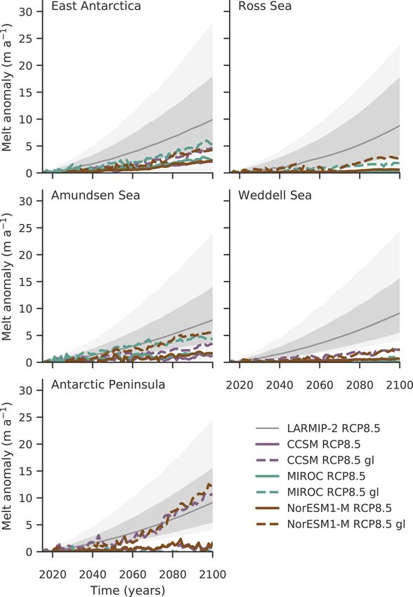
3098                                               R. Reese et al.: Role of history and ocean forcing in Antarctic projections

Sheet Model Intercomparison Project for CMIP6 (ISMIP6;             depth-dependent, nonlocal parameterization and a depth-
Nowicki et al., 2016, 2020; Seroussi et al., 2020) and the         dependent, local parameterization have been proposed (Jour-
Linear Antarctic Response Model Intercomparison Project            dain et al., 2019) that both mimic a quadratic dependency
(LARMIP-2; Levermann et al., 2014, 2020) projects. In IS-          of melt rates on thermal forcing (Holland et al., 2008). As
MIP6, a protocol for Antarctic projections was developed           an alternative, more complex modules that capture the basic
and ice sheet model responses to oceanic and atmospheric           physical processes within ice-shelf cavities have been devel-
forcing from selected CMIP5 models (Barthel et al., 2020)          oped recently (Lazeroms et al., 2018; Reese et al., 2018a).
were gathered and compared for the first time. As a first step     We here analyze results as submitted to ISMIP6 that apply
of ISMIP6, initMIP-Antarctica did test the effect of differ-       the Potsdam Ice-shelf Cavity mOdel (PICO; Reese et al.,
ent model initializations on idealized experiments (Seroussi       2018a), which extends the ocean box model (Olbers and
et al., 2019). While the response of the ice sheet to surface      Hellmer, 2010) for application in three-dimensional ice sheet
mass balance forcing was similar among the models, they            models. The model has been tested and compared to other
showed very different responses to basal melt rate changes.        parameterizations for an idealized geometry (Favier et al.,
Similarly, in ISMIP6 a large spread in model projections is        2019). In this case, the induced ice sheet response matches
found, with ice volume changes from −7.8 to 30.0 cm of             the response driven by a three-dimensional ocean model. In
sea level equivalent (SLE) under the highest greenhouse gas        contrast to ISMIP6, the LARMIP-2 experiments are forced
emission scenario (Representative Concentration Pathway            by basal melt rate changes directly. Scaling factors between
RCP8.5) with the largest uncertainties coming from ocean-          global mean temperature changes and Antarctic subsurface
induced melt rates, the calibration of melt rates and the ice      temperature changes are determined from CMIP5 models.
dynamic response to oceanic changes. The ISMIP6 projec-            These are used to generate ocean temperature forcing under
tions are given with respect to the control simulation, hence      different RCP scenarios emulated from MAGICC6.0 RCP re-
not considering current trends of mass loss.                       alizations (Meinshausen et al., 2011). Sub-shelf melt rates
   Sea level estimates in ISMIP6 are in many cases sub-            are assumed to increase by 7 to 16 m a−1 per degree Celsius
stantially lower than the ocean-driven mass loss projected         of subsurface ocean warming, based on Jenkins (1991) and
by LARMIP-2. In LARMIP-2, the sea level contribution of            Payne et al. (2007).
the Antarctic Ice Sheet is emulated from step-forcing exper-          Here we compare simulations with the Parallel Ice Sheet
iments using linear response function theory (Winkelmann           Model as submitted to ISMIP6 with results obtained follow-
and Levermann, 2013). A median mass loss of 17 cm with a           ing the LARMIP-2 protocol and analyze (1) the effect of the
likely range from 9 to 36 cm and a very likely range of 6 to       oceanic forcing and (2) the effect of a historic simulation
58 cm is found. In contrast to ISMIP6, atmospheric changes,        preceding the projections. In Sect. 2 we describe the meth-
which add mass gains between −2.5 and 84.5 mm SLE to the           ods used and the initial configurations of PISM. This is fol-
ice sheet depending on the CMIP5 forcing, are not consid-          lowed by an analysis of the experiments for ISMIP6 with
ered in LARMIP-2, and we here also focus on the dynamic,           only ocean forcing applied and the results obtained when
ocean-driven response of the ice sheet.                            following the LARMIP-2 protocol in Sect. 3. These are com-
   In projections of the future Antarctic sea level contribution   pared and discussed in Sects. 4 and 5.
following the ISMIP6 and LARMIP-2 protocols, oceanic
forcing is obtained from subsurface ocean conditions in
general circulation models, e.g., from results of the Cou-         2   Methods
pled Model Intercomparison Project Phase 5 (CMIP5; Tay-
lor et al., 2012). This approach takes into account that sub-      We use the comprehensive, thermo-mechanically coupled
shelf melt rates are mainly driven by inflow of ocean water        Parallel Ice Sheet Model (PISM; Bueler and Brown, 2009;
masses at depth (Jacobs et al., 1992). However, CMIP5 mod-         Winkelmann et al., 2011; The PISM authors, 2019) which
els do not include ice-shelf cavities and related feedbacks that   employs a superposition of the shallow-ice and shallow-shelf
might increase the future oceanic forcing on the ice shelves       approximations (Hutter, 1983; Morland, 1987; MacAyeal,
(Timmermann and Goeller, 2017; Donat-Magnin et al., 2017;          1989). We apply a power-law relationship between shallow-
Bronselaer et al., 2018; Golledge et al., 2019). Ocean temper-     shelf approximation (SSA) basal sliding velocities and basal
atures from CMIP5 models therefore have to be extrapolated         shear stress with a Mohr–Coulomb criterion relating the yield
into ice-shelf cavities (Jourdain et al., 2019). Alternatively,    stress to parameterized till material properties and the effec-
output from high-resolution models that resolve ocean dy-          tive pressure of the overlaying ice on the saturated till (Bueler
namics on the continental shelf and within the ice-shelf cavi-     and Pelt, 2015). Basal friction and sub-shelf melting are lin-
ties could be used (e.g., Hellmer et al., 2012; Naughten et al.,   early interpolated on a sub-grid scale around the grounding
2018).                                                             line (Feldmann et al., 2014). In order to improve the approxi-
   The subsurface ocean forcing informs parameteriza-              mation of driving stress across the grounding line, the surface
tions that provide melt rates underneath the ice shelves           gradient is calculated using centered differences of the ice
for ice sheet models. For the ISMIP6 experiments, a                thickness across the grounding line. We apply eigen-calving

The Cryosphere, 14, 3097–3110, 2020                                                    https://doi.org/10.5194/tc-14-3097-2020
R. Reese et al.: Role of history and ocean forcing in Antarctic projections                                                  3099

(Levermann et al., 2012) in combination with the removal of          in grounded ice thickness is 166 m (165 m) in the Amund-
ice that is thinner than 50 m or extends beyond present-day          sen Sea, 188 m (189 m) in the Ross Sea, 167 m (167 m) in
ice fronts (Fretwell et al., 2013).                                  the Weddell Sea and 250 m (250 m) for the entire conti-
                                                                     nent. The mean grounding line deviation is 12 km (13 km)
2.1   Initial configurations                                         in the Amundsen Sea, 24 km (24 km) in the Ross Sea, 14 km
                                                                     (15 km) in the Weddell Sea and 17 km (17 km) in the entire
We use two model configurations of the Antarctic Ice Sheet           domain.
that were submitted to ISMIP6, one with a preceding his-
toric simulation from 1850 to 2014 and one starting from a           2.2   Experiments
steady state. Both configurations share the same initialization
procedure: starting from Bedmap2 ice thickness and topogra-          We here present experiments based on the ISMIP6,
phy (Fretwell et al., 2013), a spin-up is run for 400 000 years      LARMIP-2 and initMIP protocols that were done for both
with constant geometry to obtain a thermodynamic equilib-            initial configurations. A list of all experiments is given in
rium with present-day climate on 16 km resolution. Based             Table S1 in the Supplement. The initMIP experiments em-
on this, an ensemble of simulations with varying model pa-           ploy idealized forcing designed to test the model response to
rameters is run for several thousand years towards dynamic           simplified forcing of the surface mass balance (experiment
equilibrium on 8 km horizontal resolution. The simulations           “asmb”) and the basal mass balance (experiment “abmb”),
employ 121 vertical layers with a quadratic spacing from             which increase linearly for 50 years and are kept constant
13 m at the ice shelf base to 100 m towards the surface.             afterwards (Seroussi et al., 2019).
We vary parameters of PICO (heat exchange coefficient γT                For LARMIP-2, constant step-forcing perturbations of the
and overturning coefficient C) as well as the minimum till           basal mass balance (4, 8 and 16 m a−1 ) are applied in five
friction angle in the parameterized till material properties         Antarctic regions (Antarctic Peninsula, East Antarctica, Ross
(8min ). The initial configuration is selected in two steps: after   Sea, Amundsen Sea, Weddell Sea). From the modeled sea
5000 years of model simulation, five candidates that com-            level response, linear response functions are derived that can
pare best to present-day observations of ice geometry and            be used to emulate the model’s response to arbitrary melt
speed (Fretwell et al., 2013; Rignot et al., 2011) are selected      forcing.
and continued. After 12 000 years the best fit equilibrium re-          The ISMIP6 protocol prescribes atmospheric and oceanic
sult was selected among them and used as initial configura-          forcing from CMIP5 models. We use the forcing data pro-
tion for the projections; see Fig. S1 in the Supplement. We          vided by ISMIP6 for (1) NorESM1-M for RCP8.5 (Bentsen
assess the ensemble members at each step using a scoring             et al., 2013; Iversen et al., 2013), (2) MIROC-ESM-CHEM
method (Pollard et al., 2016; Albrecht et al., 2020) that tests      for RCP8.5 (Watanabe et al., 2011), (3) NorESM1-M for
for root-mean-square deviation to present-day ice thickness,         RCP2.6 and (4) CCSM4 for RCP8.5 (Gent et al., 2011) as
ice-stream velocities, and deviations in grounded and floating       further described in experiments 1–4 in Nowicki et al. (2020)
area, and the average distance to the observed grounding line        and Seroussi et al. (2020). To be consistent with LARMIP-2,
position. We lay a specific focus on the Amundsen region,            we here only apply the ocean forcing in projections and keep
Filchner–Ronne and Ross ice shelves, by additionally eval-           the surface mass balance constant.
uating each indicator for these drainage basins individually.           We run experiments for both initial configurations with ∗
The historic simulation is based on the same initial steady          indicating simulations starting from the pseudo-steady state
state configuration and additionally applies atmospheric and         in 2015, INIT∗ . The control experiments for both initial con-
oceanic forcing over the period from 1850 to 2014 as de-             figurations employ constant climate conditions as described
scribed below. The initial state for the experiments with-           in the following two subsections.
out historic simulation, hereafter referred to as INIT∗ , and
the initial configuration after the historic simulation, here-       2.3   Atmosphere forcing
after referred to as INIT, are shown in Fig S2. The INIT∗
configuration is very close to a steady-state with ice vol-          Surface mass balance and ice surface temperatures for the
ume change rates being 5 mm over 85 years while the INIT             initial configuration without historic forcing are from RAC-
state is out of balance with ice volume change rates being           MOv2.3p2 (1986 to 2005 averages, Van Wessem et al.,
−1.5 cm over 85 years; see Table 1. The INIT state in 2014           2018), remapped from 27 km resolution. The historic simula-
after the historic simulation scores very similar to the best-       tion is started from the same conditions with historic surface
scoring initial configuration INIT∗ . For example, the root-         mass balance and surface temperature changes following the
mean-square deviation in stream velocity in the Amundsen             NorESM1-M simulation as suggested by ISMIP6 (Bentsen
Sea region is 113 m a−1 for INIT (improved from 116 m a−1            et al., 2013). The historic forcing from NorESM1-M is nor-
for INIT∗ ), in the Ross Sea 35 m a−1 (compared to 33 m a−1 ),       malized to its initial period (1950–1980) and the anomalies
in the Weddell Sea 47 m a−1 (38 m a−1 ) and in the entire do-        are then added to the constant climatology from RACMO.
main 290 m a−1 (262 m a−1 ). The root-mean-square deviation          Since the provided data start in 1950, surface mass balance

https://doi.org/10.5194/tc-14-3097-2020                                                   The Cryosphere, 14, 3097–3110, 2020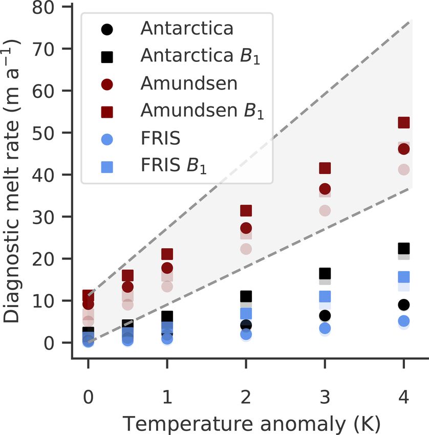
3100                                              R. Reese et al.: Role of history and ocean forcing in Antarctic projections

and temperatures are constant between 1850 and 1949. Over
that period, the aggregated yearly surface mass balance is
very similar to the RACMO climatology, as shown in Fig. S3.
   In contrast to ISMIP6, where surface mass balance and
surface temperature changes are driven by CMIP5 data, we
here keep surface conditions – in line with LARMIP-2 – con-
stant throughout the projections. Note that due to changes
in the ice sheet extent, surface mass balance integrated over
the entire ice sheet might change slightly; see Table 1. Sur-
face mass balance and temperatures in the projections that
start from the pseudo-steady-state INIT∗ are given by the         Figure 1. Historic simulation and projections of the Antarctic Ice
RACMO climatology. For the projections based on the his-          Sheet driven by ISMIP6 ocean forcing. Shown is the evolution of
toric simulation we created a new climatology to account          the sea level contribution (a) for the historic simulation relative to
for increases in surface mass balance and temperatures in         its control simulation and (b) for the projections with respect to the
the historic simulation. We avoid using exceptionally high        control simulations, in centimeters of sea level equivalent (SLE).
or low values that arise from interannual variability at a spe-   Experiments are initialized either from a historic run (solid lines)
cific snapshot in time by using the 1995 to 2014 average of       or from the initial state (dashed lines) and forced with changes in
the respective fields.                                            ocean temperature and salinity from ISMIP6 experiment nos. 1 to 4
                                                                  with the respective CMIP5 model indicated in the legend.
2.4    Ocean forcing
                                                                     Ocean temperature and salinity forcing is calculated from
Sub-shelf melt rates are calculated by PICO which extends
                                                                  CMIP5 models using an anomaly approach as suggested for
the ocean box model by Olbers and Hellmer (2010) for ap-
                                                                  ISMIP6 (Barthel et al., 2020; Jourdain et al., 2019). We av-
plication in three-dimensional ice sheet models (Reese et al.,
                                                                  erage these values over 400 to 800 m depth to obtain suitable
2018a). It mimics the vertical overturning circulation in ice-
                                                                  input for PICO. The historic forcing is based on NorESM1-M
shelf cavities and has two model parameters that apply for
                                                                  (as suggested for ISMIP6) and anomalies are normalized to
all Antarctic ice shelves simultaneously: C related to the
                                                                  the initial period (here 1850–1900), similar to the atmosphere
strength of the overturning circulation and γT related to the
                                                                  forcing. A new ocean climatology for the experiments start-
vertical heat exchange across the ice–ocean boundary layer.
                                                                  ing from the historic simulation is obtained from the 1995 to
We here use parameters C = 1 × 10⁶ m6 s−1 kg−1 and γT =
                                                                  2014 average conditions.
3 × 10⁻⁵ m s−1 that were found to yield realistic melt rates
                                                                     For LARMIP-2, we add melt rate anomalies to the under-
in comparison to present-day estimates (Reese et al., 2018a;
                                                                  lying PICO melt rates in different Antarctic regions as de-
Rignot et al., 2013). The value of γT is slightly higher than
                                                                  scribed in Levermann et al. (2020). Using linear response
the reference value as an outcome of the ensemble study; see
                                                                  theory, the probability distribution of the sea level contribu-
Fig. S1 in the Supplement.
                                                                  tion for RCP8.5 is then calculated following the LARMIP-2
   We initialize PICO with an ocean data compilation from
                                                                  protocol.
the World Ocean Atlas 2018 pre-release (Locarnini et al.,
2018; Zweng et al., 2018) and Schmidtko et al. (2014). PICO
is driven by ocean temperature and salinity averaged over         3     Results
the depth of the continental shelf within each drainage basin.
The data from the WOA2018 pre-release are processed by            We present here (1) the results for the two initial configu-
determining the relevant depth from bathymetric access to         rations submitted to ISMIP6 and (2) the sea level estimates
ice-shelf cavities. In Dronning Maud Land (PICO basins 2          for RCP8.5 obtained following the LARMIP-2 and ISMIP6
to 5), where ocean temperatures have a warm bias due to the       experiments based on the historic configuration.
lack of data along narrow continental shelves, values from
Schmidtko et al. (2014) were used. Using the currently ob-        3.1    Initial configurations and historic simulation
served “warm” conditions in the Amundsen Sea, we found
that region to collapse in the initial ensemble irrespective of   The two initial configurations for 2015, one based on a
basal sliding parameters. As this region is out of balance to-    pseudo-equilibrium and one on a historic simulation from
day due to oceanic forcing (e.g., Konrad et al., 2018; Shep-      1850 to 2014, do not differ much in terms of state variables
herd et al., 2018), it would be inconsistent to initialize our    such as ice thickness, volume or speed (see Sect. 2.1). How-
model by running it towards equilibrium over several thou-        ever, the configurations have opposed change rates: INIT∗
sand years applying constant present-day climate forcing. We      has a small tendency to gain mass and INIT is clearly out of
hence reduced temperatures in the Amundsen Sea to “cold”          balance and loses mass (compare the control simulations in
conditions (−1.25 ◦ C; Jenkins et al., 2018).                     Table 1). Over the historic period, the ice sheet thins along its

The Cryosphere, 14, 3097–3110, 2020                                                    https://doi.org/10.5194/tc-14-3097-2020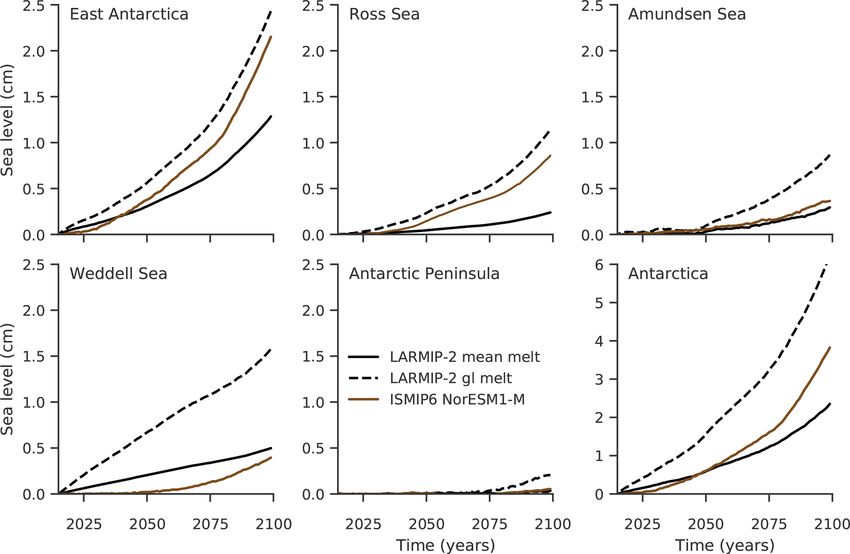
R. Reese et al.: Role of history and ocean forcing in Antarctic projections                                                          3101

margins through increased sub-shelf melting and at the same
time thickens in the interior due to more snowfall. These
signals are smaller than 50 m over grounded regions; see
Fig. S2. The thinning of ice shelves around the margins and
subsequent reduction of buttressing cause the ice streams and
ice shelves to slightly speed up over the historic simulation.
The sensitivity of the modeled ice thickness and velocities
to the historic forcing is smaller than the sensitivity to dif-
ferent parameters in the initial ensemble; see Fig. S1. Over-
all, continent-wide aggregated basal mass balance decreases
more strongly than the aggregated surface mass balance in-
creases, leading to mass loss of 3.6 mm SLE between 1850
and 2014 in comparison to the historic control simulation;
see Figs. 1 and S3. This is smaller than the observed mass
loss of 7.6 ± 3.9 mm SLE between 1992 and 2017 (Shepherd
et al., 2018).                                                        Figure 2. A preceding historic simulation increases the susceptibil-
   The patterns of present-day thickness changes (here 2014)          ity of the ice sheet to ocean forcing in projections. Shown is the
are more realistic in the historic configuration INIT than for        mass loss in simulations started directly from the initial state com-
the pseudo-equilibrium state INIT∗ . Furthermore, the high-           pared to simulations based on a historic run. The mass loss in 2100
est mass losses are simulated in the Amundsen Sea and Tot-            is given with respect to the control simulation, after 85 years of
ten regions, which agrees with observations (Shepherd et al.,         applying the ocean forcing from ISMIP6 experiment nos. 1 to 4
                                                                      with the respective emission scenario/CMIP5 model indicated on
2018). Both initial configurations are further compared to
                                                                      the x axis.
other model configurations and to present-day ice thickness
and velocities in Seroussi et al. (2020).

3.2   Comparison to initMIP Antarctica                                comparison to the control simulation, which is substantially
                                                                      smaller than previous estimates of Antarctica’s sea level con-
Results from the idealized surface mass balance experi-               tribution (e.g., DeConto and Pollard, 2016; Golledge et al.,
ment “asmb” as described in initMIP Antarctica (Seroussi              2019; Edwards et al., 2019) or expert judgment (Bamber
et al., 2019) are very similar for initial states with both           et al., 2019). Furthermore, we find that the historic simula-
119 mm SLE of mass gains for the “historic” configura-                tion makes the configuration more susceptible to ocean forc-
tion INIT and 118 mm SLE for the “cold-start” configuration           ing; see Fig. 2. Ocean-driven mass loss in comparison to the
INIT∗ after 85 years of simulation with respect to the con-           control run is increased by about 50 % (factor of 1.5) when
trol simulations; see Table 1. This is close to the response          starting from the historic simulation in contrast to the cold-
of the different models that participated in initMIP Antarc-          start simulation.
tica which showed mass gains between 125 and 186 mm SLE
after 100 years.                                                      3.4   LARMIP-2 basal melt rate forcing experiments
   For the idealized basal melt rate experiment “abmb” from
initMIP Antarctica, both states are also quite similar with           In LARMIP-2, sea level probability distributions from the
mass loss of 43 and 40 mm SLE after 85 years; see Table 1.            Antarctic Ice Sheet are derived using linear response func-
In comparison, in Seroussi et al. (2019) a model spread of            tions as described in Levermann et al. (2020). The response
13 to 427 mm SLE after 100 years is reported. Results for             functions are derived from experiments in which constant
both configurations presented here are close to the median of         basal melt rate forcing is applied for five different regions of
model results for both experiments tested in initMIP Antarc-          Antarctica. We here perform the same experiments for both
tica.                                                                 configurations described in Sect. 2.
                                                                         We find that for all regions the ice sheet response compares
3.3   ISMIP6 ocean-forcing experiments                                with the responses found in LARMIP-2 as, for example, in
                                                                      the PISM-PIK contribution that is based on a different ini-
We here compare simulations for both initial configurations           tial state with 4 km horizontal resolution and that does not
that are driven by ocean forcing from the ISMIP6 experiment           apply subgrid melting; compare Fig. 3 with Fig. 4 from Lev-
nos. 1 to 4 (see Sect. 3.3; Seroussi et al., 2020). In general, the   ermann et al. (2020). A detailed comparison of both PISM-
ice sheet’s mass loss increases with stronger ocean forcing as        PIK contributions is given in Table S2. Similar to the IS-
projected for RCP8.5 in comparison to RCP2.6; see Fig. 1.             MIP6 simulations, the experiments show different responses
The highest losses for RCP8.5 are found for NorESM1-M.                for the two initial configurations, especially in the Weddell
The magnitude of mass loss ranges from 1.4 to 4.0 cm SLE in           Sea, East Antarctica and Amundsen Sea regions. The overall

https://doi.org/10.5194/tc-14-3097-2020                                                      The Cryosphere, 14, 3097–3110, 2020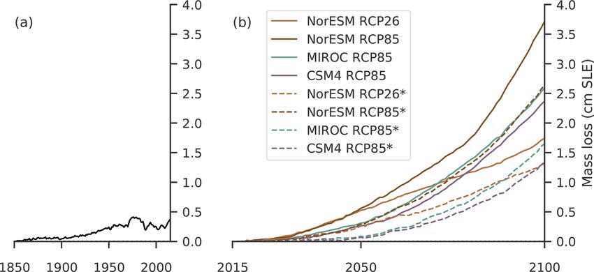
3102 R. Reese et al.: Role of history and ocean forcing in Antarctic projections
Table 1. Mass loss and evolution of surface and basal mass balance in ISMIP6 simulations. All values, except for the ctrl simulations, are
relative to the respective control simulation.
Experiments 1SMB 1BMB 1SMB+1BMB Sea level contribution
Gt a−1 Gt a−1 Gt a−1 mm SLE
historic ctrl 3 8 11 −5.2
historic 65 −428 −362 3.6
ctrl −17 8 −9 14.9
asmb 764 −28 735 −119.3
abmb −51 −538 −590 42.7
NorESM RCP85 −41 −1071 −1112 39.6
MIROC RCP85 −24 −748 −772 27.6
NorESM RCP26 −23 −107 −130 18.7
CCSM4 RCP85 −31 −790 −821 25.3
ctrl∗ 4 19 23 −4.9
asmb∗ 770 −25 746 −117.5
abmb∗ −56 −562 −618 39.8
NorESM RCP85∗ −40 −1024 −1064 27.1
MIROC RCP85∗ −30 −778 −808 17.0
NorESM RCP26∗ −25 −79 −104 13.5
CCSM4 RCP85∗ −28 −787 −815 13.7
Experiments without the historic run are indicated by ∗ . Changes in basal and surface mass balance from the first
to the last time steps in the experiments (i.e., from 1850 to 2014 in the historic run and from 2015 to 2100 in the
other experiments).
Table 2. Percentiles of the probability distribution of the sea level the PISM-PIK contribution of LARMIP-2 has a very likely
contribution from Antarctica under the RCP8.5 climate scenario range of 7 to 48 cm SLE, a likely range of 11 to 31 cm SLE
from 2015 to 2100, estimated following the LARMIP-2 protocol. and a median of 19 cm SLE for the 21st century. The result-
ing sea level probability distribution is hence in line with the
Percentile SLE, INIT∗ SLE, INIT Difference estimates presented in LARMIP-2.
(cm) (cm) (%)
5.0 % 3.3 3.5 5.5
16.6 % 8.5 9.1 6.8 4 Discussion
50.0 % 17.2 18.3 6.4
83.3 % 33.9 35.8 5.7 In the following, we compare the results found in the ISMIP6
95.0 % 52.8 55.6 5.3 and LARMIP-2 experiments and discuss the role of the ocean
forcing and of the historic simulation.
4.1 Comparison of LARMIP-2 and ISMIP6 sea level
difference is smaller than in the ISMIP6 experiments for the projections
stronger forcing applied here.
Following the procedure in LARMIP-2, we derive re- The projected mass loss in LARMIP-2 is an order of mag-
sponse functions from the idealized experiments for the five nitude larger than the ocean-driven mass loss in our ISMIP6
Antarctic regions. We then convolve the response function experiments for RCP8.5; see Sect. 3. In order to understand
with basal melt rate forcing, given in Fig. 4, to obtain a this difference better, we here investigate the ocean forcing
probability distribution of the future sea level contribution in more detail.
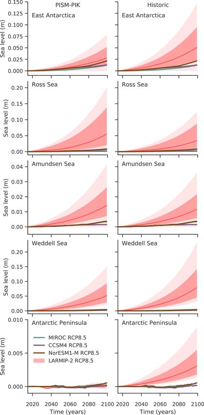
for RCP8.5 which is given in Fig. 5. The ocean-driven mass Both intercomparison projects, ISMIP6 and LARMIP-2,
loss from 2015 to 2100 has a very likely range of 3.5 to are based on CMIP5 model subsurface ocean temperature
55.6 cm SLE, a likely range of 9.1 to 35.8 cm SLE and a me- changes (Levermann et al., 2014; Barthel et al., 2020; Jour-
dian of 18.3 cm SLE (percentiles 5 to 95, 16.6 to 83.3, and dain et al., 2019). While they are directly applied in IS-
50, respectively; see Table 2). Similar to the ISMIP6 simu- MIP6, they are used to derive a scaling between global
lations, these results obtained for the historic initial configu- mean temperatures and Antarctic subsurface temperatures in
ration are larger than the results for the steady-state configu- LARMIP-2. While minor differences in ocean forcing might
ration, with increases between 5 % and 7 %. In comparison, occur due to different processing steps, a more significant
The Cryosphere, 14, 3097–3110, 2020 https://doi.org/10.5194/tc-14-3097-2020R. Reese et al.: Role of history and ocean forcing in Antarctic projections 3103
Figure 3. Mass loss of the different regions in Antarctica (indicated
on the y axis) driven by constant LARMIP-2 basal melt rate forc-
ing. For the experiments from the LARMIP-2 protocol we show the Figure 4. Projected basal melt rate changes in the different Antarc-
changes in volume above flotation initialized from a historic simu- tic regions from LARMIP-2 and in the ISMIP6 contribution forced
lation (solid line) and from the initial state directly (dashed line, in- with NorESM1-M, CCSM and MIROC ocean changes under
dicated by ∗ ). Mass loss is shown relative to the respective control RCP8.5. In LARMIP-2 spatially constant basal melt rate forcing
simulation. From the response of the ice sheet to a constant melt is applied with corresponding very likely ranges (5th to 95th per-
rate forcing over 200 years, a response function is derived which centiles, light gray shading), likely ranges (66th percentile around
then serves to emulate the sea level contribution under various cli- the median, dark gray shading) and median (gray line) for the
mate scenarios. This figure is similar to Fig. 4 in Levermann et al. RCP8.5 scenario. In the ISMIP6 contribution, basal melt rates are
(2020). calculated by PICO, which shows higher increases close to the
grounding line (PICO box 1, indicated by “gl”) than averaged over
the ice shelves. Figure is similar to Fig. 3 in Levermann et al. (2020).
difference is that the LARMIP-2 experiments are driven by
basal melt rate changes emulated from the forcing, while in
the ISMIP6 simulations ocean forcing is translated into basal PICO along the grounding line are hence an upper limit for
melt rates via sub-shelf melt parameterizations, in our case the comparison to the LARMIP-2 forcing while the shelf-
PICO. wide averaged changes provide a lower limit. Overall, we
Figure 4 shows projected basal melt rates and their un- find that in the ISMIP6 simulations, basal melt rates increase
certainty ranges for RCP8.5 used in LARMIP-2 together more in regions with smaller ice shelves than in the Ross and
with the basal melt rate changes in the ISMIP6 simulations. Weddell seas. Furthermore, we find that the basal melt rate
Note that LARMIP-2 assumes constant changes in basal melt changes in our ISMIP6 contribution in all Antarctic regions
rates over the entire ice shelf. In contrast, since PICO mim- are located in the lower range (percentiles) of the LARMIP-
ics the vertical overturning circulation in ice-shelf cavities, 2 forcing. Only for the Antarctic Peninsula do PICO melt
basal melt rates in the ISMIP6 simulations increase more rates along the grounding line increase more strongly than
strongly along the grounding line (in PICO’s first box) and the median in LARMIP-2 for NorESM1-M and MIROC. For
less towards the ice shelf front. The melt rate changes in all other regions, melt rate changes along the grounding line
https://doi.org/10.5194/tc-14-3097-2020 The Cryosphere, 14, 3097–3110, 20203104 R. Reese et al.: Role of history and ocean forcing in Antarctic projections
and for the Weddell Sea, they are lower than the very likely
range (5th to 95th percentiles). Shelf-wide changes are gen-
erally smaller than the likely range; for the Weddell Sea and
the Antarctic Peninsula they are also smaller than the very
likely range.
This is consistent with the mass loss in the ISMIP6 sim-
ulations being lower than the likely range of LARMIP-2 for
almost all regions; see Fig. 5. These findings are underlined
by the direct comparison with the PISM-PIK contribution to
LARMIP-2 which is based on a different initial setup; see
Sect. 3.4. Note that basal melt rate changes in East Antarctica
seem similar in Fig. 4 for NorESM1-M and MIROC but mass
loss is higher for NorESM1-M, because the ocean forcing in
the ISMIP6 simulations varies across the different ice shelves
in East Antarctica. While there is stronger ocean warming
in Dronning Maud Land and Amery in the MIROC forcing,
the ocean warms substantially more in the Totten region for
NorESM1-M. The higher vulnerability of the Totten region
then causes higher overall mass loss.
In Fig. 6 we assess for each region the mass loss by ap-
plying the response functions to the corresponding PICO
melt rate changes driven by NorESM1-M ocean forcing,
once averaged over the entire ice shelves and once close to
the grounding lines. When comparing the respective mass
loss with the ISMIP6 simulation, we find that indeed the
changes at the grounding line provide an upper limit while
the changes over the entire ice shelf provide a lower limit for
the actual mass loss.
Overall, we find that mass losses in the ISMIP6 projec-
tions are generally lower than the likely range in LARMIP-2,
and in the Weddell Sea losses are smaller than the very likely
range, as the basal melt rate changes in the LARMIP experi-
ments are an order of magnitude higher than those estimated
with PICO and ISMIP6 forcing.
4.2 Role of ocean forcing and basal melt rate sensitivity
In order to gain a better understanding of the conversion of
ocean forcing to basal melt rates in LARMIP-2 and in our
ISMIP6 contribution, we further analyze the sensitivity to
Figure 5. Projections of Antarctica’s sea level contribution under
ocean warming.
the RCP8.5 climate scenario for the different Antarctic regions for
LARMIP-2 and for the ISMIP6 experiments driven by NorESM1-
We perform step-forcing experiments for both initial con-
M, MIROC and CCSM4 ocean forcing. The very likely ranges (5th figurations and diagnose the effect on basal melt rates; see
to 95th percentiles, light red shading), likely ranges (percentiles Fig. 7. Ocean temperatures are increased by 0.5, 1, 2, 3 and
16.6 to 83.3, dark red shading) and the respective median (50th per- 4 ◦ C, and the corresponding basal melt rates for constant ice-
centile, red lines) of mass loss are shown for (left panels) the PISM- shelf geometries are diagnosed using PICO. We find that the
PIK simulations submitted to LARMIP-2 (Levermann et al., 2020) sensitivity in the Amundsen Sea region is comparatively high
and for comparison (right panels) estimated following LARMIP-2 with about 10 m a−1 K−1 , while the sensitivity in the Wed-
for the setup as submitted to ISMIP6. dell Sea is lower with about 1.5 m a−1 K−1 , which yields for
the entire Antarctic ice shelves an overall sensitivity of about
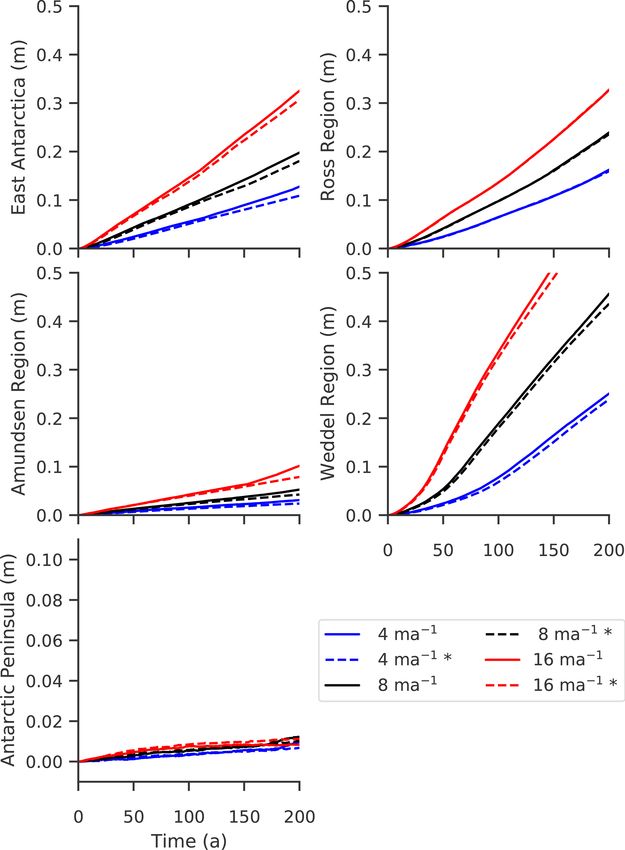
2.2 m a−1 K−1 . The sensitivities for melting close to the
are smaller than the median in LARMIP-2 (50th percentile). grounding line are as expected a bit higher: 10.5 m a−1 K−1
For the Amundsen Sea region, they lie within the likely range for the Amundsen Sea region, 3.9 m a−1 K−1 for the Wed-
(percentiles 16.6 to 83.3). For East Antarctica and the Ross dell Sea and 5.3 m a−1 K−1 on average for all Antarctic ice
Sea, they are around the lower margin of the likely range, shelves. In both cases, the Antarctic-wide sensitivity is sub-
The Cryosphere, 14, 3097–3110, 2020 https://doi.org/10.5194/tc-14-3097-2020R. Reese et al.: Role of history and ocean forcing in Antarctic projections 3105
Figure 6. Projections using PICO forced with NorESM1-M ocean conditions compared to projection obtained by the response function.
The response function is derived for the INIT configuration. It is applied to the basal melt rate forcing from PICO using average conditions
underneath the shelves in the corresponding sector (generally an underestimation) and using the melting at the grounding line (generally an
overestimation) from Fig. 4.
stantially lower than the sensitivity used in LARMIP-2. In
the latter study, a sensitivity between 7 and 16 m a−1 K−1 ,
based on Jenkins (1991) and Payne et al. (2007), is assumed
to translate ocean forcing into sub-shelf melt rates. This is
consistent with our findings in the previous section that in the
ISMIP6 simulations mass loss from the Antarctic Ice Sheet,
and especially from the regions that drain the large Filchner–
Ronne and Ross ice shelves, is smaller than the likely range
estimated following the LARMIP-2 protocol. Jourdain et al.
(2019) report that a different tuning of the ISMIP6 basal melt
parameterization to fit observations in the Amundsen Sea
(from Dutrieux et al., 2014; Jenkins et al., 2018) substan-
tially increases the sensitivity to ocean changes and Seroussi
et al. (2020) find that this enhances the sea level contribution
by a factor of 6.
Since the sensitivity in PICO depends on the parameters Figure 7. Sensitivity of basal melt rates to ocean temperatures in
used, with the overturning coefficient C affecting the sensi- PICO. Diagnosed from the historic configuration (opaque) and the
tivity in large ice shelves and the heat exchange coefficient cold-start configuration (transparent) in 2015 using step-wise ocean
γT affecting the sensitivity in small ice shelves, a different temperature increases. Dots show shelf-wide averages while boxes
tuning could improve basal melt rate sensitivities and thereby indicate the basal melt rates close to the grounding lines (in PICO
lead to higher mass losses in the ISMIP6 experiments. A con- box B1 ). The dashed gray lines indicate the sensitivity estimates
sistency of sub-shelf melt rates with present-day observations used in Levermann et al. (2020).
could be achieved by introducing additional degrees of free-
dom through temperature corrections that reflect uncertain-
ties in ocean properties, as for example used in Lazeroms Few observations exist for targeted tuning of the sensitiv-
et al. (2018) and Jourdain et al. (2019). In addition, tuning ity of basal melt rate parameterizations to ocean tempera-
to realistic melt rates close to the grounding lines (in PICO’s tures; hence the use of dynamic modeling of the ocean cir-
first box) is potentially more important than fitting shelf-wide culation in ice-shelf cavities could be explored. We estimate
melt rates (e.g., Goldberg et al., 2019; Reese et al., 2018b). that the sensitivity in Seroussi et al. (2017) varies between 6
and 16 m a−1 K−1 with an average of 9.4 m a−1 K−1 over the
https://doi.org/10.5194/tc-14-3097-2020 The Cryosphere, 14, 3097–3110, 20203106 R. Reese et al.: Role of history and ocean forcing in Antarctic projections
first 20 years of model simulation, which would be in line historic simulation, where the local freezing point at the ice
with the sensitivities used in LARMIP-2; see Fig. S5. shelf base near the grounding line is decreased due to its pres-
Note that we provide linear estimates of the sensitivity of sure dependence. Hence more heat is available for melting
PICO in the discussion above, while Holland et al. (2008) the ice-shelf base, which also shows an increased sensitiv-
report a quadratic dependency of melt rates on thermal forc- ity to ocean changes; see Fig. 7. In particular for lower tem-
ing. They also discuss that the sensitivity depends on ice peratures, PICO shows a nonlinear sensitivity of melt rates
shelf cavity properties such as the slope of the ice-shelf draft to ocean temperatures, as discussed in Reese et al. (2018a).
and shape of the ice shelf and that sensitivities are gener- Further investigations would be required to disentangle the
ally higher close to the grounding line. Further factors that reasons for the increased susceptibility to ocean warming af-
influence ocean circulation, such as bathymetry, also affect ter the historic simulation, also considering the strength of
the ocean sensitivity. While PICO takes into account that the forcing applied.
not all heat content of the ocean water masses that enter the The sea level contribution over the historic period from
cavity might be used for melting, it does not capture three- 1850 to 2014 is 3.6 mm in comparison to the control sim-
dimensional circulations in ice-shelf cavities that play a role ulation. This is smaller than the reported mass loss of the
in particular for larger ice shelves such as Filchner–Ronne. Antarctic Ice Sheet that amounts to 7.6 ± 3.0 mm SLE be-
tween 1992 and 2017 (Shepherd et al., 2018). An improved
4.3 Role of historic trajectory of the Antarctic Ice Sheet understanding of the basal melt rate sensitivity, potential bi-
ases in the atmospheric or oceanic forcing, and an extension
We find that while the historic simulation has no large ef- of the scoring with observed patterns of thickness changes
fect on the initial sea level volume (the overall difference be- would allow for performing “hindcasting” experiments that,
ing 1.6 mm SLE), it affects the mass loss in the projections. in a next step, could inform future projections.
A number of reasons might cause the simulations starting
from the historic configuration (INIT) to be more vulnera-
ble to ocean forcing: both simulations have different initial 5 Conclusions
trends of the sea level relevant volume and rates of ice thick-
ness change. These trends, or the different geometry after In this study we compare sea level projections for RCP8.5
the historic simulation, might make the configuration more from the Antarctic Ice Sheet as submitted to ISMIP6, using
susceptible to ocean forcing, for example through nonlinear the PICO basal melt rate parameterization and constant sur-
changes in ice-shelf buttressing. In addition, the historic sim- face mass balance forcing, and projections derived following
ulation might have pushed the ice sheet (closer) to a local the LARMIP-2 protocol that scales global temperatures to
instability that evolves in the projections. Figure S6 shows subsurface temperatures and melt rates, both using the Paral-
the mass loss rates for all simulations presented in Sect. 3.3. lel Ice Sheet Model. Overall, we find that the sea level con-
In general, the rates are higher in the simulations based on tribution driven by ocean forcing in ISMIP6 is smaller than
the historic configuration, and these differences increase over the likely range of the sea level probability distribution in
time. In the RCP8.5 simulation forced with NorESM1-M LARMIP-2. This difference can be explained by the com-
ocean conditions, at around year 2075 a clear shift to sub- parably low sensitivity of melt rates to ocean temperature
stantially higher differences is visible. We hypothesize that changes for the parameter tuning in PICO in comparison to
this could be linked to a local instability that is kicked off LARMIP-2 where a sensitivity of 7 to 16 m a−1 K−1 is used
for the simulations starting from the historic configuration that we found to be consistent with a coupled simulation
but not for those starting from the pseudo-steady state. This of Thwaites glacier (Seroussi et al., 2017). Future sea level
is less pronounced for CCSM4 and MIROC, maybe due to projections should hence carefully consider the sensitivity of
differences in the ocean forcing and regions contributing to basal melt rates to ocean changes. Additional observations
sea level rise. In the idealized experiments for LARMIP-2 of ocean conditions and ocean-induced melt rates in combi-
(Fig. 3), differences in simulations starting from the two ini- nation with ocean modeling are needed to better constrain
tial states arise in particular in East Antarctica, the Weddell this sensitivity for the diverse ice-shelf cavities in Antarc-
Sea and the Amundsen Sea, less in the Ross Sea. The effect tica. Furthermore, we find that while the initial state result-
of the historic simulation is reduced for the stronger basal ing from a historic simulation from 1850 to 2014 is virtu-
melt rate forcing applied in the LARMIP-2 experiments, with ally indistinguishable from a steady-state simulation, the his-
mass loss increases in the projections between 5 % and 7 %. toric simulation increases the projected mass loss in 2100
Furthermore, the ice sheet’s response might have changed by up to 50 %. This means that not only the currently com-
after the historic simulation due to changes in boundary con- mitted sea level contribution in projections but also the ef-
ditions. Moreover, changes in the ice sheet state could result fect of the historic forcing on the ice sheet’s susceptibility
since, for instance, the underlying equation system depends to ocean changes should be considered. Hindcasting experi-
nonlinearly on the three-dimensional temperature field. The ments, which reproduce observed thinning rates and ice loss
grounding line retreats slightly into deeper regions during the over the past decades, would be valuable to better constrain
The Cryosphere, 14, 3097–3110, 2020 https://doi.org/10.5194/tc-14-3097-2020R. Reese et al.: Role of history and ocean forcing in Antarctic projections 3107
model parameters and improve confidence in projections. PLR-1644277. The authors gratefully acknowledge the European
Hence, further investigations are needed to assess the sen- Regional Development Fund (ERDF), the German Federal Ministry
sitivity of basal melting to ocean temperatures for basal melt of Education and Research and the Land Brandenburg for support-
parameterizations and the role of historical forcing and initial ing this project by providing resources for the high-performance
conditions in future sea level projections. computer system at the Potsdam Institute for Climate Impact Re-
search. Computer resources for this project have also been pro-
vided by the Gauss Centre for Supercomputing, Leibniz Supercom-
puting Centre (http://www.lrz.de, last access: 16 July 2020) under
Code and data availability. Model outputs from the simulations
project IDs pr94ga and pn69ru. Ronja Reese is supported by the
for ISMIP6 described in this paper as well as forcing datasets will
Deutsche Forschungsgemeinschaft (DFG) by grant WI4556/3-1 and
be made available via the ISMIP6 project with a digital object iden-
through the TiPACCs project that receives funding from the Euro-
tifier (Nowicki et al., 2020). LARMIP-2 code and data are available
pean Union’s Horizon 2020 Research and Innovation program un-
via the project (Levermann et al., 2020). The PISM code, the PISM
der grant agreement no. 820575. Torsten Albrecht is supported by
simulations and the scripts to analyze the simulations and create
the Deutsche Forschungsgemeinschaft (DFG) in the framework of
the figures are available at https://doi.org/10.5281/zenodo.3903343
the priority program “Antarctic Research with comparative investi-
(Reese et al., 2020). The processing of the World Ocean Atlas pre-
gations in Arctic ice areas” by grants WI4556/2-1 and WI4556/4-1
release data is described in the Bachelor thesis by Lena Nicola
and in the framework of the PalMod project (FKZ: 01LP1925D),
(2019) and will be shared upon request.
supported by the German Federal Ministry of Education and Re-
search (BMBF) as a Research for Sustainability initiative (FONA).
Hélène Seroussi was supported by grants from NASA’s Cryospheric
Supplement. The supplement related to this article is available on- Science and Modeling, Analysis, Predictions programs.
line at: https://doi.org/10.5194/tc-14-3097-2020-supplement. We would like to thank the anonymous reviewers for their helpful
comments on the manuscript and the editor Douglas Brinkerhoff for
handling the review process. We are grateful to Matthias Mengel
Author contributions. RR and AL designed the study. All authors for supporting the development of the scoring scheme and PISM
contributed to the interpretation of the results. RR performed the analysis tools as well as Lena Nicola for providing the processed
model simulations and carried out the analysis. AL calculated the ocean input data.
response function and provided data for the LARMIP-2 compari-
son. TA and RR developed the scoring scheme for the PISM simu-
lations. HS analyzed the melt sensitivity in the coupled simulations. Financial support. This research has been supported by
RR prepared the manuscript with contributions from all authors. the Deutsche Forschungsgemeinschaft (DFG) (grant nos.
WI4556/3-1, WI4556/2-1, and WI4556/4-1), the NASA (grant
no. NNX17AG65G), the NSF (grant nos. PLR-1603799 and
Competing interests. Helene Seroussi is an editor of the special is- PLR-1644277), and the Gauss Centre for Supercomputing/Leibniz
sue “The Ice Sheet Model Intercomparison Project for CMIP6 (IS- Supercomputing Centre (grant nos. pr94ga and pn69ru).
MIP6)”. The authors declare that no other competing interests are
present. The publication of this article was funded by the
Open Access Fund of the Leibniz Association.
Special issue statement. This article is part of the special issue
“The Ice Sheet Model Intercomparison Project for CMIP6 (IS- Review statement. This paper was edited by Douglas Brinkerhoff
MIP6)”. It is not associated with a conference. and reviewed by two anonymous referees.
Acknowledgements. We thank the Climate and Cryosphere (CliC)
effort, which provided support for ISMIP6 through sponsoring of
References
workshops, hosting the ISMIP6 website and wiki, and promoting
ISMIP6. We acknowledge the World Climate Research Programme,
Albrecht, T., Winkelmann, R., and Levermann, A.: Glacial-cycle
which, through its Working Group on Coupled Modelling, coordi-
simulations of the Antarctic Ice Sheet with the Parallel Ice
nated and promoted CMIP5. We thank the climate modeling groups
Sheet Model (PISM) – Part 2: Parameter ensemble analy-
for producing and making available their model output, the Earth
sis, The Cryosphere, 14, 633–656, https://doi.org/10.5194/tc-14-
System Grid Federation (ESGF) for archiving the CMIP data and
633-2020, 2020.
providing access, the University at Buffalo for ISMIP6 data distri-
Bamber, J. L., Oppenheimer, M., Kopp, R. E., Aspinall, W. P., and
bution and upload, and the multiple funding agencies who support
Cooke, R. M.: Ice sheet contributions to future sea-level rise
CMIP5 and ESGF. We thank the ISMIP6 steering committee, the
from structured expert judgment, P. Natl. Acad. Sci. USA, 116,
ISMIP6 model selection group and the ISMIP6 dataset preparation
11195–11200, 2019.
group for their continuous engagement in defining ISMIP6. This
Barthel, A., Agosta, C., Little, C. M., Hattermann, T., Jourdain,
is ISMIP6 contribution no. 15. Development of PISM is supported
N. C., Goelzer, H., Nowicki, S., Seroussi, H., Straneo, F., and
by NASA grant NNX17AG65G and NSF grants PLR-1603799 and
Bracegirdle, T. J.: CMIP5 model selection for ISMIP6 ice sheet
https://doi.org/10.5194/tc-14-3097-2020 The Cryosphere, 14, 3097–3110, 20203108 R. Reese et al.: Role of history and ocean forcing in Antarctic projections model forcing: Greenland and Antarctica, The Cryosphere, 14, thickness datasets for Antarctica, The Cryosphere, 7, 375–393, 855–879, https://doi.org/10.5194/tc-14-855-2020, 2020. https://doi.org/10.5194/tc-7-375-2013, 2013. Bentsen, M., Bethke, I., Debernard, J. B., Iversen, T., Kirkevåg, Frieler, K., Clark, P. U., He, F., Buizert, C., Reese, R., Ligten- A., Seland, Ø., Drange, H., Roelandt, C., Seierstad, I. A., berg, S. R., Van Den Broeke, M. R., Winkelmann, R., and Hoose, C., and Kristjánsson, J. E.: The Norwegian Earth Sys- Levermann, A.: Consistent evidence of increasing Antarctic tem Model, NorESM1-M – Part 1: Description and basic evalu- accumulation with warming, Nat. Clim. Change, 5, 348–352, ation of the physical climate, Geosci. Model Dev., 6, 687–720, https://doi.org/10.1038/nclimate2574, 2015. https://doi.org/10.5194/gmd-6-687-2013, 2013. Gent, P. R., Danabasoglu, G., Donner, L. J., Holland, M. M., Hunke, Bronselaer, B., Winton, M., Griffies, S. M., Hurlin, W. J., Rodgers, E. C., Jayne, S. R., Lawrence, D. M., Neale, R. B., Rasch, P. J., K. B., Sergienko, O. V., Stouffer, R. J., and Russell, J. L.: Change Vertenstein, M., Worley, Z.-L., and Yang, M. Z.: The commu- in future climate due to Antarctic meltwater, Nature, 564, 53–58, nity climate system model version 4, J. Climate, 24, 4973–4991, https://doi.org/10.1038/s41586-018-0712-z, 2018. 2011. Bueler, E. and Brown, J.: Shallow shelf approximation as a “sliding Goldberg, D., Gourmelen, N., Kimura, S., Millan, R., and Snow, K.: law” in a thermomechanically coupled ice sheet model, J. Geo- How accurately should we model ice shelf melt rates?, Geophys. phys. Res., 114, F03008, https://doi.org/10.1029/2008JF001179, Res. Lett., 46, 189–199, 2019. 2009. Golledge, N. R., Keller, E. D., Gomez, N., Naughten, K. A., Bueler, E. and van Pelt, W.: Mass-conserving subglacial hydrology Bernales, J., Trusel, L. D., and Edwards, T. L.: Global envi- in the Parallel Ice Sheet Model version 0.6, Geosci. Model Dev., ronmental consequences of twenty-first-century ice-sheet melt, 8, 1613–1635, https://doi.org/10.5194/gmd-8-1613-2015, 2015. Nature, 566, 65–72, https://doi.org/10.1038/s41586-019-0889-9, DeConto, R. M. and Pollard, D.: Contribution of Antarctica 2019. to past and future sea-level rise, Nature, 531, 591–597, Hellmer, H. H., Kauker, F., Timmermann, R., Determann, J., and https://doi.org/10.1038/nature17145, 2016. Rae, J.: Twenty-first-century warming of a large Antarctic ice- Donat-Magnin, M., Jourdain, N. C., Spence, P., Le Sommer, J., shelf cavity by a redirected coastal current, Nature, 485, 225– Gallée, H., and Durand, G.: Ice-Shelf Melt Response to Chang- 228, https://doi.org/10.1038/nature11064, 2012. ing Winds and Glacier Dynamics in the Amundsen Sea Sector, Holland, P. R., Jenkins, A., and Holland, D. M.: The Response of Ice Antarctica, J. Geophys. Res.-Oceans, 122, 10206–10224, 2017. Shelf Basal Melting to Variations in Ocean Temperature, J. Cli- Dutrieux, P., De Rydt, J., Jenkins, A., Holland, P. R., Ha, H. K., Lee, mate, 21, 2558–2572, https://doi.org/10.1175/2007JCLI1909.1, S. H., Steig, E. J., Ding, Q., Abrahamsen, E. P., and Schröder, 2008. M.: Strong sensitivity of Pine Island ice-shelf melting to climatic Hutter, K. E.: Theoretical glaciology: material science of ice and the variability, Science, 343, 174–178, 2014. mechanics of glaciers and ice sheets, Springer, vol. 1, 1983. Edwards, T. L., Brandon, M. A., Durand, G., Edwards, N. R., Iversen, T., Bentsen, M., Bethke, I., Debernard, J. B., Kirkevåg, Golledge, N. R., Holden, P. B., Nias, I. J., Payne, A. J., Ritz, C., A., Seland, Ø., Drange, H., Kristjansson, J. E., Medhaug, and Wernecke, A.: Revisiting Antarctic ice loss due to marine I., Sand, M., and Seierstad, I. A.: The Norwegian Earth ice-cliff instability, Nature, 566, 58–64, 2019. System Model, NorESM1-M – Part 2: Climate response Favier, L., Jourdain, N. C., Jenkins, A., Merino, N., Durand, G., and scenario projections, Geosci. Model Dev., 6, 389–415, Gagliardini, O., Gillet-Chaulet, F., and Mathiot, P.: Assess- https://doi.org/10.5194/gmd-6-389-2013, 2013. ment of sub-shelf melting parameterisations using the ocean– Jacobs, S., Hellmer, H., Doake, C. S. M., Jenkins, A., ice-sheet coupled model NEMO(v3.6)–Elmer/Ice(v8.3) , Geosci. and Frolich, R. M.: Melting of ice shelves and the Model Dev., 12, 2255–2283, https://doi.org/10.5194/gmd-12- mass balance of Antarctica, J. Glaciol., 38, 375–387, 2255-2019, 2019. https://doi.org/10.3189/S0022143000002252, 1992. Feldmann, J., Albrecht, T., Khroulev, C., Pattyn, F., and Levermann, Jenkins, A.: Ice shelf basal melting: Implications of a simple math- A.: Resolution-dependent performance of grounding line motion ematical model, Filchner-Ronne Ice Shelf Programme Report, 5, in a shallow model compared with a full-Stokes model accord- 32–36, 1991. ing to the MISMIP3d intercomparison, J. Glaciol., 60, 353–360, Jenkins, A., Shoosmith, D., Dutrieux, P., Jacobs, S., Kim, https://doi.org/10.3189/2014JoG13J093, 2014. T. W., Lee, S. H., Ha, H. K., and Stammerjohn, S.: West Fretwell, P., Pritchard, H. D., Vaughan, D. G., Bamber, J. L., Bar- Antarctic Ice Sheet retreat in the Amundsen Sea driven rand, N. E., Bell, R., Bianchi, C., Bingham, R. G., Blanken- by decadal oceanic variability, Nat. Geosci., 11, 733–738, ship, D. D., Casassa, G., Catania, G., Callens, D., Conway, H., https://doi.org/10.1038/s41561-018-0207-4, 2018. Cook, A. J., Corr, H. F. J., Damaske, D., Damm, V., Ferracci- Jourdain, N. C., Asay-Davis, X., Hattermann, T., Straneo, F., oli, F., Forsberg, R., Fujita, S., Gim, Y., Gogineni, P., Griggs, Seroussi, H., Little, C. M., and Nowicki, S.: A protocol for calcu- J. A., Hindmarsh, R. C. A., Holmlund, P., Holt, J. W., Jacobel, lating basal melt rates in the ISMIP6 Antarctic ice sheet projec- R. W., Jenkins, A., Jokat, W., Jordan, T., King, E. C., Kohler, tion, The Cryosphere, 14, 3111–3134, https://doi.org/10.5194/tc- J., Krabill, W., Riger-Kusk, M., Langley, K. A., Leitchenkov, 14-3111-2020, 2020. G., Leuschen, C., Luyendyk, B. P., Matsuoka, K., Mouginot, Konrad, H., Shepherd, A., Gilbert, L., Hogg, A. E., McMillan, M., J., Nitsche, F. O., Nogi, Y., Nost, O. A., Popov, S. V., Rignot, Muir, A., and Slater, T.: Net retreat of Antarctic glacier ground- E., Rippin, D. M., Rivera, A., Roberts, J., Ross, N., Siegert, ing lines, Nat. Geosci., 11, 258–262, 2018. M. J., Smith, A. M., Steinhage, D., Studinger, M., Sun, B., Lazeroms, W. M. J., Jenkins, A., Gudmundsson, G. H., and van de Tinto, B. K., Welch, B. C., Wilson, D., Young, D. A., Xiangbin, Wal, R. S. W.: Modelling present-day basal melt rates for Antarc- C., and Zirizzotti, A.: Bedmap2: improved ice bed, surface and tic ice shelves using a parametrization of buoyant meltwater The Cryosphere, 14, 3097–3110, 2020 https://doi.org/10.5194/tc-14-3097-2020
You can also read