Soil moisture and streamflow deficit anomaly index: an approach to quantify drought hazards by combining deficit and anomaly - Natural Hazards and ...
←
→
Page content transcription
If your browser does not render page correctly, please read the page content below
Nat. Hazards Earth Syst. Sci., 21, 1337–1354, 2021
https://doi.org/10.5194/nhess-21-1337-2021
© Author(s) 2021. This work is distributed under
the Creative Commons Attribution 4.0 License.

Soil moisture and streamflow deficit anomaly index: an approach to
quantify drought hazards by combining deficit and anomaly
Eklavyya Popat1 and Petra Döll1,2
1 Institute   of Physical Geography, Goethe University Frankfurt, Frankfurt am Main, Germany
2 Senckenberg     Leibniz Biodiversity and Climate Research Centre Frankfurt (SBiK-F), Frankfurt am Main, Germany

Correspondence: Eklavyya Popat (popat@em.uni-frankfurt.de)

Received: 7 August 2020 – Discussion started: 19 August 2020
Revised: 15 March 2021 – Accepted: 23 March 2021 – Published: 3 May 2021

Abstract. Drought is understood as both a lack of water (i.e.,      1   Introduction
a deficit compared to demand) and a temporal anomaly in
one or more components of the hydrological cycle. Most
drought indices, however, only consider the anomaly aspect,         According to the Australian Bureau of Meteorology,
i.e., how unusual the condition is. In this paper, we present       “drought is a prolonged, abnormally dry period when the
two drought hazard indices that reflect both the deficit and        amount of available water is insufficient to meet our normal
anomaly aspects. The soil moisture deficit anomaly index,           use” (BoM, 2018). This definition describes drought as both
SMDAI, is based on the drought severity index, DSI (Cam-            an anomaly (“less water than normal”) and a deficit (“less
malleri et al., 2016), but is computed in a more straightfor-       water than required”), reflecting general non-expert notions
ward way that does not require the definition of a mapping          of drought. However, most experts define drought only as
function. We propose a new indicator of drought hazard for          an anomaly, for example, as “a lack of water compared to
water supply from rivers, the streamflow deficit anomaly in-        normal conditions which can occur in different components
dex, QDAI, which takes into account the surface water de-           of the hydrological cycle” (Van Loon et al., 2016, p. 3633).
mand of humans and freshwater biota. Both indices are com-          Assuming that humans and other biota are accustomed to
puted and analyzed at the global scale, with a spatial res-         seasonal variations in water availability in the form of pre-
olution of roughly 50 km, for the period 1981–2010, using           cipitation, soil moisture, streamflow or groundwater storage,
monthly time series of variables computed by the global wa-         droughts are mostly defined by the deviation of a water quan-
ter resources and the model WaterGAP 2.2d. We found that            tity at a specific point in time (e.g., precipitation in May
the SMDAI and QDAI values are broadly similar to values of          2005) from its long-term mean or median (e.g., of all May
purely anomaly-based indices. However, the deficit anomaly          precipitation values during the reference period 1981–2010).
indices provide more differentiated spatial and temporal pat-       It is further assumed for most drought hazard indicators that
terns that help to distinguish the degree and nature of the ac-     humans and other biota are used to interannual variability.
tual drought hazard to vegetation health or the water supply.       Therefore, drought is not defined by a percentage deviation
QDAI can be made relevant for stakeholders with different           but rather by using percentiles (e.g., precipitation in May
perceptions about the importance of ecosystem protection,           2005 is less than the 10th percentile of all May precipita-
by adapting the approach for computing the amount of water          tion values during the reference period) or by standardized
that is required to remain in the river for the well-being of the   drought indicators where the anomaly is divided by the stan-
river ecosystem. Both deficit anomaly indices are well suited       dard deviation. Anomaly-based drought indicators that in-
for inclusion in local or global drought risk studies.              dicate less water than normal include the standardized pre-
                                                                    cipitation index (SPI) (Mckee et al., 1993), the standard-
                                                                    ized precipitation evapotranspiration index (SPEI) (Vicente-
                                                                    Serrano et al., 2010; Bergez et al., 2013), the China Z index
                                                                    (CZI) (Wu et al., 2001) and, for streamflow drought, the stan-

Published by Copernicus Publications on behalf of the European Geosciences Union.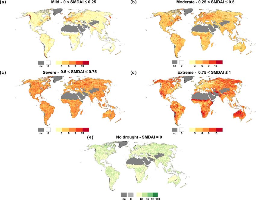
1338                                                E. Popat and P. Döll: Soil moisture and streamflow deficit anomaly index

dardized streamflow index (SSFI) (Modarres, 2007) and the           irrigation is the largest water demand sector, accounting for
percentile-based low-flow index by Cammalleri et al. (2017).        more than 60 % of total surface water withdrawals (Müller
   Some researchers have quantified drought by only con-            Schmied et al., 2021; Döll et al., 2014). To date, however,
sidering the deficit aspect of drought, i.e., by computing the      streamflow drought indicators only describe the anomaly of
difference between an optimal water quantity and the actual         streamflow but do not indicate whether there is enough water
quantity (“less water than required”). Deficit-based indica-        in the river to meet water demand. Thus, to assess the risk
tors have only been derived for assessing drought risk for          of drought for human water supply from rivers, an indica-
vegetation, as optimal water quantities can be defined by ei-       tor that combines the anomaly of streamflow conditions with
ther the field capacity of the soil (Sridhar et al., 2008) or po-   a deficit, with respect to water demand, is desirable. In this
tential evapotranspiration. For the latter, the deficit is com-     way, the locations and times where the human water supply
puted either as the difference between potential evapotran-         is at risk can be identified.
spiration and precipitation (Hogg et al., 2013) or between             Differently from anomaly-based streamflow drought in-
potential and actual evapotranspiration. A drawback of these        dicators, a combined analysis of streamflow anomaly and
deficit-based drought hazard indicators is that they indicate       deficit requires time series information of both streamflow
strong drought in arid and (semi)arid regions, even though          and water demand. This information is available from global
the vegetation in these regions is adapted to generally lower       water resources and uses models such as WaterGAP with a
soil moisture (Cammalleri et al., 2016). Deficit-based indi-        spatial resolution of 0.5◦ (55 km by 55 km at the Equator) and
cators cannot be meaningfully derived for the variable pre-         a monthly temporal resolution (Alcamo et al., 2003; Müller
cipitation only as the definition of an optimal precipitation       Schmied et al., 2021). Up to the present time, macro-scale
amount depends on the user of the precipitation water. It is,       drought risk assessments have included the demand for water
however, conceptually meaningful to determine deficits for          as vulnerability indicators by using a country’s average ratio
human water supply based on the variable streamflow, defin-         of water withdrawal to water availability (e.g., Meza et al.,
ing the deficit as the difference between the demand for water      2020).
from the river and the actual streamflow. To the best of our           In this study, we introduce and relate two drought hazard
knowledge, streamflow drought has not, as yet, been charac-         indicators that combine both the deficit and anomaly aspects:
terized by a deficit-based drought indicator.                       one for soil moisture drought and the other for streamflow
   Two notable attempts in identifying and bringing together        drought. In the soil moisture deficit anomaly index (SMDAI),
both the anomaly and deficit aspects are the Palmer drought         the deficit is calculated as the difference between the soil
severity index (PDSI) (Palmer, 1965) and the drought sever-         moisture at field capacity (which allows optimal and non-
ity index (DSI) (Cammalleri et al., 2016). PDSI is a stan-          water-limited plant growth) and the actual soil moisture. The
dardized index developed to quantify the cumulative deficit         SMDAI slightly modifies and simplifies the DSI introduced
of moisture supply in the form of precipitation compared            by Cammalleri et al. (2016). Another difference from Cam-
to demand in the form of potential evapotranspiration. Its          malleri et al. (2016) is that the SMDAI is computed glob-
strengths and weakness have been well investigated by Dai           ally, using the output of WaterGAP, rather than just for Eu-
et al. (2004) and is extensively used in the USA to indi-           rope. The streamflow deficit anomaly index QDAI is, to our
cate meteorological droughts (Heim, 2002). DSI indicates            knowledge, the first ever streamflow drought indicator that
soil moisture drought by combining the soil moisture deficit        combines both the anomaly and deficit aspects of streamflow
(compared to the situation in which plant evapotranspira-           drought. In the case of QDAI, the deficit is computed by com-
tion is not constrained by soil moisture availability) and the      paring actual streamflow to the combined human and envi-
anomaly of the deficit, thus indicating rare events in which        ronmental surface water demand per grid cell. QDAI focuses
plants suffer from water stress. An anomaly-based soil mois-        on determining the drought hazard for the water supply for
ture drought may, however, be unsuitable for indicating a           humans, including domestic, industrial, and irrigation water
drought hazard for vegetation as, in areas with high soil mois-     demand. QDAI is constructed similarly to SMDAI and com-
ture in most years, the low interannual variability and, thus,      puted globally using WaterGAP. Whether QDAI should be
the standard deviation would indicate a strong drought haz-         called a drought hazard indicator, or a combined drought haz-
ard in years with unusually low soil moisture values that are,      ard and vulnerability indicator, is up for discussion. However,
nevertheless, still close to the optimal values and do not cause    for global-scale drought risk assessments, gridded QDAI val-
any water stress for the plants (Cammalleri et al., 2016).          ues can be meaningfully combined with country-scale vul-
   Similar to the demand for soil water by plants, humans           nerability indicators of, for example, coping capacity.
have a demand for water from rivers in situations where                In Sect. 2, we describe (a) how water demand, streamflow,
they rely on river water for their water supply. About three-       surface water use and soil moisture are computed by Water-
quarters of global water withdrawals for irrigation, cooling        GAP 2.2d (Müller Schmied et al., 2021) and (b) the meth-
of thermal power plants, manufacturing and domestic use, to-        ods for calculating SMDAI and QDAI. In Sect. 3, spatial and
talling about 3700 km3 yr−1 in the first decade of this century,    temporal patterns of SMDAI and QDAI are presented. In
are sourced from surface water (Döll et al., 2014). Globally,       Sect. 4, we analyze the components of SMDAI and QDAI,

Nat. Hazards Earth Syst. Sci., 21, 1337–1354, 2021                                 https://doi.org/10.5194/nhess-21-1337-2021
E. Popat and P. Döll: Soil moisture and streamflow deficit anomaly index                                                       1339

compare SMDAI to DSI, compare QDAI to a standardized                Schmied et al., 2014; Döll et al., 2003; Alcamo et al., 2003).
streamflow indicator (SSFI), and discuss the limitations of         The soil is represented as one water storage compartment that
the study. Finally, we draw conclusions in Sect. 5.                 is characterized by (1) soil water capacity (Smax ), which is
                                                                    computed as the product of land cover, specific rooting depth
                                                                    and soil water capacity in the upper meter, and (2) soil tex-
2     Methods and data                                              ture, which affects groundwater recharge (Müller Schmied
                                                                    et al., 2014). The temporal development of soil moisture (S)
2.1    Global-scale simulation of soil moisture, soil water         is computed from the balance of inflows (precipitation and
       capacity, streamflow and human water abstraction             snowmelt minus interception by the canopy) and outflows
                                                                    (actual evapotranspiration and total runoff from the land). To-
In this study, we use the outputs of the latest version             tal runoff from the land fraction of the grid cell is then par-
of the global hydrological and water use model Water-               titioned into the fast surface and subsurface runoff and the
GAP 2.2d (Müller Schmied et al., 2021). WaterGAP consists           diffuse groundwater recharge. Both components are subject
of three major components: the water use models, the linked         to so-called fractional routing to the various other storages
groundwater–surface water use (GWSWUSE) model and the               within the 0.5◦ grid cell, which include the groundwater as
global hydrological model (WGHM). The water use mod-                well as lakes, wetlands, man-made reservoirs and rivers (Döll
els compute water use in the five sectors: household, man-          et al., 2014). Streamflow (Qant ) in each grid cell depends on
ufacturing, cooling of thermal power plants, livestock and          the runoff generated within the cell, inflow from upstream
irrigation. Household and manufacturing water use is com-           grid cells as well as human water abstractions and takes into
puted based on national statistics (Flörke et al., 2013). The       account the impact of man-made reservoirs.
amount of water required for cooling of thermal power plants            WGHM is calibrated to match long-term annual observed
is calculated based on the location, type and size of power         streamflows at the outlets of 1319 drainage basins that cover
plants and the annual time series of thermal electricity pro-       ∼ 54 % of the global drainage area, following the calibration
duction (Flörke et al., 2013). Irrigation water use is com-         principles provided by Müller Schmied et al. (2014), Hunger
puted based on information on the irrigated area and climate        and Döll (2008), and Döll et al. (2003). In validation stud-
for each grid cell. The irrigation model first computes cell-       ies against time series of observed streamflows, WaterGAP
specific cropping patterns and growing periods and then ir-         has been repeatedly shown to be among the best-performing
rigation consumptive water use, distinguishing only rice and        global hydrological models (Zaherpour et al., 2019, 2018;
non-rice crops (Döll and Siebert, 2002). The irrigated areas        Veldkamp et al., 2018). Nevertheless, there can be significant
change over time (Siebert et al., 2015). The globally small         mismatches between the observed and simulated seasonality
amount of livestock water use is the only temporally con-           and interannual variability.“It is found that WaterGAP can
stant water use and is determined from the number of live-          simulate the low flow percentile (Q95) very well, but it can
stock and livestock-specific water use values (Alcamo et al.,       also overestimate the return period of low streamflow” (Za-
2003). Water use for households, manufacturing and cooling          herpour et al., 2018).
of thermal power plants is constant throughout the year but             This study uses 30 years (1981–2010) of monthly
changes from year to year.                                          time series of WaterGAP gridded (0.5◦ × 0.5◦ ) outputs for
   The water use models themselves do not take into account         67 420 land grid cells covering all land areas of the globe ex-
the source of the sectoral water abstractions. This is done by      cept Greenland and Antarctica. These include (1) soil mois-
GWSWUSE, which computes monthly time series of 0.5◦                 ture (S) [mm]; (2) streamflow (Qant ) [km3 per month]; (3)
grid-cell values of human water abstractions from (1) sur-          streamflow under naturalized conditions (Qnat ) [km3 per
face water bodies (river, lakes and man-made reservoirs) and        month], assuming there are no human water abstractions or
(2) groundwater, for each of the five sectors, as well as the       man-made reservoirs; and (4) total surface water abstractions
respective net abstractions from both sources (Döll et al.,         [km3 per month]. In addition, the consistent dataset of soil
2012). A comparison of simulated annual sectoral water ab-          water capacity (Smax ) [mm] is utilized.
stractions per country to independent values from the AQUA-
STAT database of FAO showed a rather high similarity be-
tween the two datasets (Müller Schmied et al., 2021).               2.2     Computation of deficit and anomaly components of
   Taking into account the net abstractions, i.e., the difference           the soil moisture deficit anomaly index SMDAI
between water abstractions and return flows, WGHM simu-
lates, with a daily time step, the most relevant hydrological       2.2.1    Deficit
processes occurring on the continents and computes water
flows such as actual evapotranspiration, runoff, groundwa-
ter recharge and streamflow, as well as the amount of wa-           Soil moisture deficit (dsoil ) refers to the lack of water in the
ter stored in diverse compartments such as the soil and the         root zone for plants compared to optimal growing conditions
groundwater for all land areas, excluding Antarctica (Müller        assumed to occur at soil water capacity (demand for water).

https://doi.org/10.5194/nhess-21-1337-2021                                   Nat. Hazards Earth Syst. Sci., 21, 1337–1354, 2021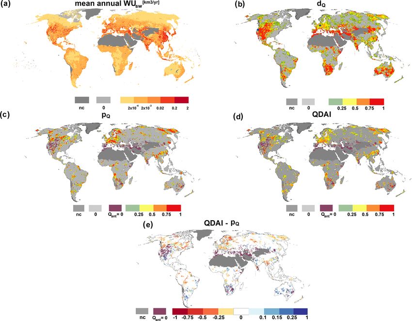
1340                                                E. Popat and P. Döll: Soil moisture and streamflow deficit anomaly index

dsoil is calculated as                                              where a, b ≥ 0 are the shape parameters, B(a, b) is the beta
          Smax − S                                                  function and B(dsoil ; a, b) is the incomplete beta function.
dsoil =            ,                                         (1)    In this form, the b supports the range of dsoil ∈ [0, 1]. In this
            Smax
                                                                    study, we could confirm the assumption made by Cammalleri
where Smax [mm] is the amount of water stored in the soil           et al. (2016) that the beta distribution function satisfactorily
between field capacity and wilting point within the plant’s         represents the distribution of dsoil , which is the same as that
root zone, and S [mm] is the actual amount of soil water (soil      of the soil moisture itself. The beta cumulative distribution
moisture). dsoil ranges from 0 (no deficit/stress) to 1 (extreme    function was fitted to dsoil values for each calendar month
deficit/stress).                                                    and grid cell (i.e., for each grid cell, 12 beta functions are
   This definition of soil moisture deficit is different from the   fitted corresponding to the 12 calendar months).
one used in Cammalleri et al. (2016, their Eq. 1) because their         Following Cammalleri et al. (2016), the next step was to
definition cannot be applied when using the global hydrolog-        derive from F a drought probability index (psoil ) that trans-
ical model WaterGAP to compute soil moisture. The deficit           lates the probability that a certain soil water deficit status is
computation according to Cammalleri et al. (2016) requires          drier than usual into the range [0, 1]. As suggested by Agnew
data on soil moisture content at the wilting point and at field     (2000), a z score of −0.84, which corresponds to a return pe-
capacity, which is not available in WaterGAP. With our ap-          riod of 5 years and a F (dsoil ) of 0.8, was assumed to be the
proach, which is consistent with the way of computing actual        threshold for drought (Table 1), for which psoil = 0. Then,
evapotranspiration from potential evapotranspiration in Wa-         the drought probability index is calculated as
terGAP, d values at low soil moisture saturation are lower
                                                                              F (dsoil ) − 0.8
than those of Cammalleri et al. (2016), while they are much         psoil =                    ,                                  (3)
higher at high soil moisture as Cammalleri et al. (2016) as-                     1 − 0.8
sume that deficits only occur if soil moisture is less than 50 %    where F (dsoil ) is the beta cumulative distribution function
of field capacity. Consequently, we identify very few months        fitted to dsoil . If the beta cumulative distribution function is
and grid cells with a deficit of zero, likely less than we would    fitted to S, then (1−F (S)) should be used instead of F (dsoil ).
if we would have implemented the deficit definition of Cam-             Cammalleri et al. (2016) calculated psoil using the mode
malleri et al. (2016).                                              instead of median as the reference for the normal status of
                                                                    dsoil . The computation of psoil from F (dsoil ) was carried out
2.2.2     Anomaly                                                   in two steps. First, for dsoil values that are greater than or
                                                                    equal to the mode, a new standardized cumulative distribu-
Assuming that vegetation is used to seasonal variations in          tion function F × (dsoil ) is computed (Eq. 3 in Cammalleri
soil moisture, the anomaly of monthly soil moisture is de-          et al., 2016). Subsequently, mapping F × (dsoil ) values rang-
termined separately for each calendar month. In the case of         ing from 0.6 to 1 onto the psoil range of [0, 1], an exponential
standardized drought indicators such as the SPI, a so-called        function (Eq. 4 in Cammalleri et al., 2016) was employed.
z score is computed separately for each calendar month (here        This exponential function was developed to fit subjectively
using, for example, 30 monthly soil moisture deficits in the        defined pairs of F × (dsoil ) and psoil (Table 1 in Cammal-
30 January months during the period 1981–2010), by stan-            leri et al., 2016). In this study, we have simplified the more
dardizing the variable using the calendar month mean and            complex approach of Cammalleri et al. (2016) by relying di-
standard deviation after translating the cumulative distribu-       rectly on F (dsoil ) for mapping F (dsoil ) onto psoil according
tion function that optimally fits the distribution of monthly       to Eq. (3). In our opinion, there is no added value in defin-
values to a normal distribution (McKee et al., 1993). Thus,         ing an arbitrary exponential mapping function for deriving an
computation of the z score assumes that the vegetation is           indicator for the probability of a drought occurrence (psoil ).
adapted to both seasonal and interannual variability. Follow-       Further, like most other drought researchers, we prefer the
ing Cammalleri et al. (2016), in this study, we express the         median to the mode, as among 30 deficit values, which are
anomaly aspect of drought not by the z score but by deriving        rational numbers, there is no true mode, i.e., no value that
a so-called drought probability index (p) that can be com-          occurs most often. The relation between the anomaly com-
bined with the deficit indicator to a deficit anomaly drought       ponent of SMDAI (i.e., psoil ) and the non-exceedance prob-
hazard index.                                                       ability of the soil moisture deficit (F (dsoil )) and the pertain-
   Computation of p also starts with identifying the prob-          ing return periods, z scores and class names, according to
ability of exceedance of a certain soil moisture deficit F .        Agnew (2000), as well as the anomaly component of DSI
Sheffield et al. (2004) found that time series of soil moisture     (p_DSI) are presented in Table 1. A comparison of psoil to
per calendar month are best represented by the beta distribu-       p_DSI values as a function of (F (dsoil )) as presented in Ta-
tion function. The cumulative density function F of the beta        ble 1 is shown in Fig. S1 in the Supplement, and the slight
distribution function can be expressed as                           differences between psoil and p_DSI, as well as DSI and SM-
                     B (dsoil ; a, b)                               DAI, computed with WaterGAP output for August 2003 at
F (dsoil ; a, b) =                    ,                      (2)    the global scale are presented in Fig. S2 in the Supplement.
                        B(a, b)

Nat. Hazards Earth Syst. Sci., 21, 1337–1354, 2021                                    https://doi.org/10.5194/nhess-21-1337-2021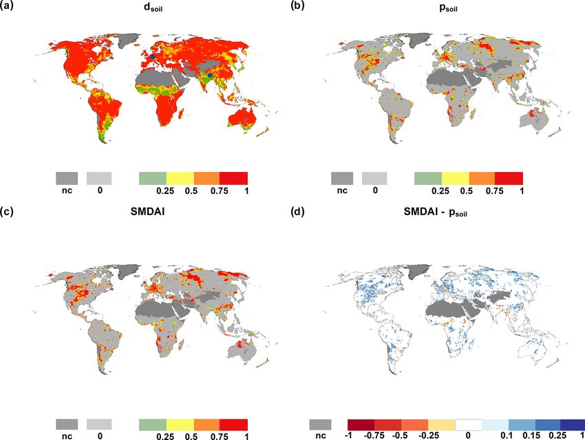
E. Popat and P. Döll: Soil moisture and streamflow deficit anomaly index                                                                1341

Table 1. Relationship of the anomaly component p of SMDAI and QDAI to the non-exceedance probability of the soil moisture deficit
(F (dsoil )) or of streamflow (F (Q)), the pertaining return periods, z scores and class names according to Agnew (2000) as well as the
p values by Cammalleri et al. (2016) to compute DSI. The class name refers to the drought conditions with z-score values that are larger
than those listed in the z-score column. The equiprobability transformation technique, first suggested by Abramowitz and Stegun (1965)
and utilized in Kumar et al. (2009) for calculation of the standardized precipitation index (SPI), is used to back-calculate F values from the
z-score values.

                        F (dsoil )/F (Q)   Return period       z score   Drought class name      p_DSI     psoil /pQ
                                                 (years)
                        0.8                             5      −0.84     Normal                       0            0
                        0.843                         6.4      −1.00     Mild                      0.04         0.21
                        0.87                          7.7      −1.12     Moderate                  0.10         0.35
                        0.9                            10      −1.28     Moderate                  0.26         0.50
                        0.933                          15      −1.50     Moderate                  0.54         0.68
                        0.95                           20      −1.64     Severe                    0.72         0.75
                        0.97                         33.3      −1.88     Severe                    0.89         0.85
                        0.9775                         40      −2.00     Severe                    0.93         0.88
                        0.99                           99      −2.33     Extreme                   0.99         0.95
                        0.995                         200      −2.57     Extreme                  0.997         0.97
                        0.998                         500      −2.88     Extreme                  0.999         0.99
                        1                               –    ∼ −4.00     Extreme                    ∼1          ∼1

For very few grid cells, SMDAI is much larger than DSI, and              Table 2. SMDAI and QDAI range corresponding to drought classes.
there are some areas where DSI is slightly larger than SM-
DAI. For the period 1981–2010, SMDAI is, averaged over                            SMDAI range/QDAI range         Drought conditions
all grid cells, 0.05 larger than DSI with according to Eq. (1).                   0 < SMDAI < 0.25               Mild
                                                                                  0.25 ≥ SMDAI < 0.5             Moderate
2.3     Computation of deficit and anomaly components of
                                                                                  0.5 ≥ SMDAI < 0.75             Severe
        the streamflow deficit anomaly index QDAI                                 SMDAI ≥ 0.75                   Extreme
2.3.1    Deficit

Similar to the soil moisture deficit, the streamflow deficit
(dQ ) is calculated as the demand for water minus the sup-               variable. dQ is, like dsoil , in the range of 0 (no deficit/stress)
ply divided by demand. It refers to the amount of streamflow             to 1 (extreme deficit/stress); if dQ is less than 0 or WUsw
that is lacking to satisfy the surface water demand of both              equals 0, then dQ is set to 0. To explore how assump-
humans and the river ecosystem. dQ is computed as                        tions about EFR and, thus, total surface water demand affect
                                                                         QDAI, we set EFR to be alternatively equal to half of Qnat ,
        (WUsw + EFR) − Qant                                              or zero (Sects. 3.2 and 4.2). These alternatives represent situ-
dQ =                        ,                                   (4)
           WUsw + EFR                                                    ations in which humans wish to protect freshwater biota less,
                                                                         or not at all, so the total surface water demands and conse-
where WUsw [km3 per month] is water abstraction from sur-                quently streamflow deficits are lower.
face water bodies, derived as the sum of water abstractions
for irrigation, livestock, cooling of thermal power plants,
manufacturing and household use. Qant [km3 per month] is                 2.3.2    Anomaly
the streamflow, and EFR [km3 per month] is the environ-
mental flow requirement, i.e., the surface water demand of               Streamflow anomaly (pQ ) is computed based on the inter-
the river ecosystem. Following Richter et al. (2012), EFR                annual variability of monthly aggregated streamflow (Qant )
is calculated for each calendar month as 80 % of the mean                values for each calendar month. We consider the anomaly
monthly streamflow under the naturalized condition (Qnat ),              of streamflow (Qant ) instead of the anomaly of the stream-
assuming that 80 % of the natural mean monthly streamflow                flow deficit (dQ ) as the temporal variability including long-
that would have occurred in the river without human water                term trends of the water demand prevented us, for most grid
use and man-made reservoirs needs to remain in the river for             cells with relevant water demand, from identifying a standard
the well-being of the river ecosystem.                                   distribution function for the time series of dQ . Furthermore,
   Differing from Smax , which represents the vegetation de-             the methodological consistency between the calculation of
mand for soil water, the streamflow demand is temporally                 pQ and psoil is maintained, as the anomaly of soil moisture

https://doi.org/10.5194/nhess-21-1337-2021                                       Nat. Hazards Earth Syst. Sci., 21, 1337–1354, 2021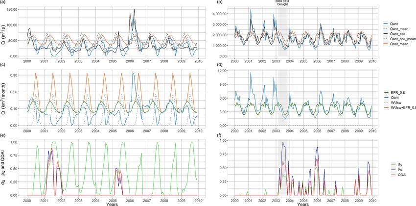
1342                                               E. Popat and P. Döll: Soil moisture and streamflow deficit anomaly index

deficit (dsoil ) is equal to the anomaly of soil moisture (S)      Schmied et al., 2014), together with grid cells in Green-
[mm].                                                              land, were not considered. For each of these grid cells and
   In some regional streamflow drought studies (Langat et al.,     each calendar month, we determined the best-fitting beta and
2019; Sharma and Panu, 2015; Lorenzo-Lacruz et al., 2010;          gamma cumulative distribution functions for monthly dsoil
López-Moreno et al., 2009), the standard cumulative dis-           and Qant , respectively, by utilizing a combination of func-
tribution function Pearson type III was used to fit monthly        tions from the R packages gamlss, gamlss.dist, extremeS-
streamflow values. However, Svensson et al. (2017) rightly         tat and fitdistrplus. However, as tested by the one-sample
pointed out that the Pearson type III distribution function        Kolmogorov–Smirnov test (KS test) at the 0.05 significance
with a lower bound at zero is reduced to the gamma distri-         level, for 27.12 % of the grid cells in the case of dsoil and
bution function. The cumulative density function F of the          39.94 % in the case of Qant , the fits were rejected for all
gamma distribution function can be expressed as                    12 calendar months. Examples of an accepted grid cell and a
                                                                   rejected grid cell of the beta distribution function are shown
                    g (Qant ; a, b)
F (Qant ; a, b) =                   ,                       (5)    in Fig. S3 in the Supplement. In the rejected grid cells, the
                        G(a)                                       probability of non-exceedance F is determined directly from
where a, b ≥ 0 are the shape parameters, G(a) is the gamma         the time series of 30 monthly values using the R function em-
function and g(Qant ; a, b) is the incomplete gamma function;      pirical cumulative distribution function (ECDF). The ECDF
in this form the gamma distribution supports d > 0. Taking         is a step function that increases by 1/30 at each of the 30 dsoil
into account that streamflow drought occurs when a certain         values of SMDAI or Qant values of QDAI (Fig. S3 left). The
streamflow value is not exceeded, while in the case of psoil       computed F value of a specific dsoil or Qant value is the frac-
a soil moisture drought occurs when a certain soil moisture        tion of all 30 dsoil or Qant values that are less than, or equal to,
deficit is exceeded, the drought probability index for stream-     the specific dsoil or Qant value. Figure S4 in the Supplement
flow drought pQ is computed as                                     shows the grid cells where ECDFs had to be used to compute
                                                                   F.
       (1 − F (Qant )) − 0.8
pQ =                         .                              (6)    2.6    Standardized streamflow index
             1 − 0.8
2.4    Combining deficit and anomaly to compute SMDAI              We compared QDAI with the well-established anomaly-
       and QDAI                                                    based drought indicator standardized streamflow index
                                                                   (SSFI) introduced by Modarres (2007). SSFI is computed
Water deficits (dsoil and dQ ) and anomalies (psoil and pQ ) are   separately for each calendar month, similar to the standard-
combined into single deficit anomaly indicators (SMDAI and         ized precipitation index (SPI) (Mckee et al., 1993), as
QDAI) based on the desired indicator characteristics as elab-
orated by Cammalleri et al. (2016). The combined drought                     Qanti − Qant
indicator should be zero if there is either no deficit- or no      SSFI =                 ,                                        (9)
                                                                                   σ
anomaly-based drought. It should be equal to p and d if p
and d are the same, while it should have lower values if           where Qanti [km3 per month] is the streamflow value at time
either d or p is close to zero. Thus, following Cammalleri         interval i, Qant is the long-term mean of the streamflow val-
et al. (2016)                                                      ues and σ is the standard deviation of the streamflow values.
            p
SMDAI = psoil · dsoil                                        (7)
                                                                   3     Results and discussions
and accordingly
        p                                                          3.1    SMDAI
QDAI = pQ · dQ .                                            (8)

   Both SMDAI and QDAI values range from 0 to 1, where             The relations between dsoil , mean monthly (dsoil_mean ), psoil
0 corresponds to no drought hazard and 1 corresponds to            and SMDAI are further clarified by the time series of
extreme drought hazard. The indicator values are put into          these variables in Fig. 1 for two grid cells with rather dif-
classes and coinciding drought classifications according to        ferent characteristics: a grid cell in Germany (42.25◦ N,
Table 2.                                                           −121.75◦ E, left panels in Fig. 1) and one in northeast India
                                                                   ( 27.25◦ N, 88.25◦ E, right panels in Fig. 1). The values of
2.5    Fitting standard cumulative functions                       dsoil in the German grid cell show, on average over the whole
                                                                   reference period, high deficits in the summer months and
Out of the total 67 420 WaterGAP land grid cells, only 57 043      low deficits only in one to two winter months (dashed grey
grid cells were considered in this study. Grid cells with bar-     line). According to the definition of psoil , an anomaly-based
ren or sparsely vegetated land cover, based on the MODIS-          drought hazard, as indicated by psoil > 0 (blue line), occurs
derived static land cover input map used in WGHM (Müller           only if the actual soil moisture deficit (green line) is much

Nat. Hazards Earth Syst. Sci., 21, 1337–1354, 2021                                 https://doi.org/10.5194/nhess-21-1337-2021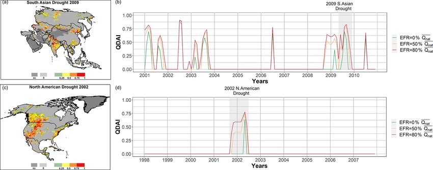
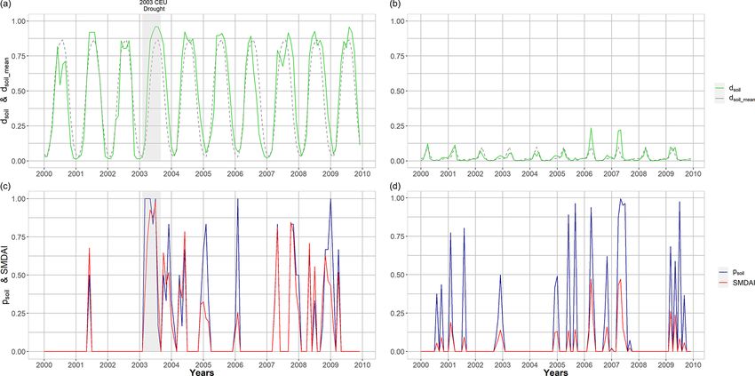
E. Popat and P. Döll: Soil moisture and streamflow deficit anomaly index                                                              1343

Figure 1. Soil moisture drought hazard: example of a time series (2000–2010) of monthly dsoil and mean seasonality of soil moisture deficit,
psoil and SMDAI for a cell in Germany (a, c) and a cell in northeast India (b, d). The central European (CEU) drought in 2003 is indicated.

higher than the mean calendar month values dsoil_mean ; per             and the monsoon areas in India (Fig. 2a). In each grid cell,
definition, this is the case in only 1 out of 5 years (Eq. 3 and        psoil is, per definition, zero in 80 % of all August months.
Table 1). According to Eq. (7), SMDAI is always between                 Therefore, in any month, approximately 80 % of the grid
psoil and dsoil . In the German cell, an anomaly-based drought          cells indicate no drought and psoil equals 0 (Fig. 2b). Only
occurred during the unusually dry, but still low-deficit, win-          grid cells with a non-zero psoil have a non-zero SMDAI
ter months of 2006, resulting in an SMDAI value that was                (Fig. 2c). For example, southeast India shows extremely high
much smaller than psoil . During the central European (CEU)             dsoil values, but as there is no anomalously high soil mois-
summer drought of 2003, SMDAI was approximately equal                   ture deficit except for a few grid cells where psoil is mostly
to psoil . Thus, SMDAI appropriately indicates that anoma-              zero, SMDAI is also mostly zero. Thus, no soil moisture
lously low soil moisture during generally wet winter months             drought hazard is indicated. The difference between SMDAI
is less of a hazard to vegetation than the same anomaly would           and psoil is shown in Fig. 2d. In most grid cells with differ-
be during generally dry summer months. The grid cell in                 ences, SMDAI is higher than psoil due to high dsoil . Focus-
northeast India is characterized by a low seasonality of soil           ing on central Europe, SMDAI (in Fig. 2c) correctly indi-
moisture and a generally very high soil water content. Even             cates the summer drought of 2003, documented in the EM-
for some unusually dry months (with high psoil ), dsoil almost          DAT International Disaster Database (http://www.emdat.be,
always remains below 0.25. Due to the low deficit, even in              last access: 11 May 2020), the European Drought Reference
cases of high psoil , SMDAI is much smaller than psoil during           database (http://www.geo.uio.no/edc/droughtdb, last access:
all drought events indicated by psoil . When comparing tem-             15 May 2020) and Spinoni et al. (2019). The location of grid
porally averaged drought hazards between the two grid cells,            cells from Fig. 1 is represented in Fig. 2a with blue points
SMDAI would indicate a relatively higher drought hazard                 drawn at the center of each grid cell. During Northern Hemi-
for the German grid cell than for the Indian grid cell, which           sphere winter months, soil moisture deficits are lower, for
would not be the case if a purely anomaly-based indicator,              example, in Europe and the eastern part of North America,
such as psoil , were used as the drought hazard indicator.              but high in most snow-dominated northern high-latitude re-
   The relationship between SMDAI, psoil and dsoil can be               gions (as no liquid water enters the soil), with correspond-
further explored by using global indicator maps for a spe-              ing effects for the relationship between psoil and SMDAI
cific month, e.g., August 2003 (Fig. 2). WaterGAP com-                  (see Fig. S5 in the Supplement showing the drought situa-
putes soil moisture deficits of 75 % or more in most grid               tion in December 1999). In Europe and the eastern part of
cells, while low deficits occur only in a few areas, where              North America, for example, SMDAI is smaller than psoil
August belongs to the rainy season, e.g., the Sahel region              (Fig. S5d).

https://doi.org/10.5194/nhess-21-1337-2021                                      Nat. Hazards Earth Syst. Sci., 21, 1337–1354, 2021
1344 E. Popat and P. Döll: Soil moisture and streamflow deficit anomaly index
Figure 2. Global maps of dsoil , psoil , SMDAI and the difference between SMDAI and psoil for August 2003. Blue points in (a) represent the
location of German and Indian grid cells from Fig. 1, and nc denotes grid cells that are not computed due to land cover.
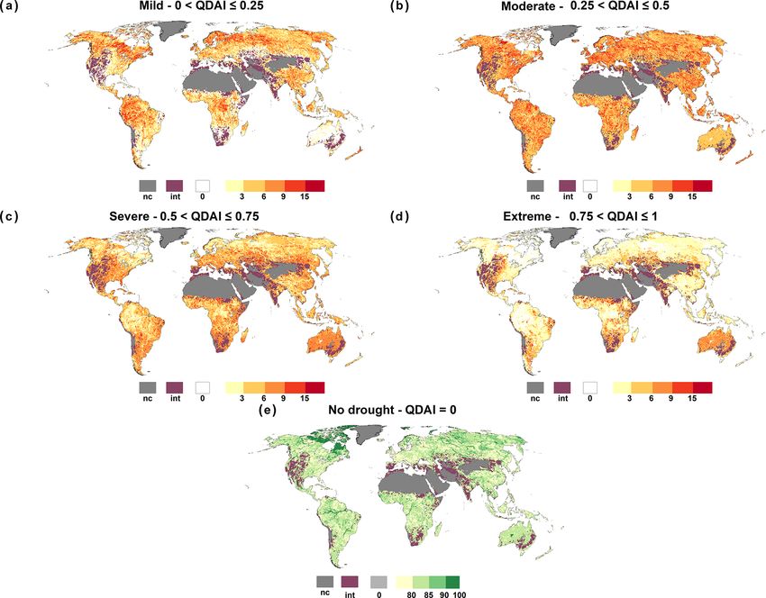
Figure 3 shows the frequency of occurrence of the four 3.2 QDAI
SMDAI drought classes specified in Table 2 and of the no-
drought condition (SMDAI = 0) during the reference period QDAI indicates the drought hazard for surface water supply
1981–2010. SMDAI is zero in about 80 % of the cases, fol- required for satisfying human water demand (WUsw ), assum-
lowing psoil as monthly soil moisture almost never reaches ing the water suppliers also take into consideration the water
the maximum soil moisture capacity. Extreme soil moisture demand by freshwater biota (EFR). The deficit component of
drought hazards occur with a relatively high frequency in QDAI (dQ ) is the relative difference between the total surface
the northwestern parts of Australia and southeastern parts water demand and streamflow, while the anomaly compo-
of Africa. Regions with mostly low soil moisture deficits, nent (pQ ) is based on the unusualness of streamflow. QDAI
such as central and eastern European countries and the east- depends on more individual variables (i.e., WUsw , Qant and
ern USA, show very low occurrence frequencies of extreme EFR) than SMDAI (i.e., S and Smax ). Figure 4 shows their re-
drought hazards and more often than other regions a moder- lation for two grid cells with different characteristics of hu-
ate drought hazard (Fig. 3b). Snow-dominated regions, such man surface water demand compared to streamflow. In the
as parts of Russia and Canada, show a relatively high fre- grid cell in the western USA, where streamflow of the Kla-
quency of extreme soil moisture droughts due to the high math River is observed in Keno (42.25◦ N, −121.75◦ E, left
values of simulated soil moisture deficits created by the lack panels of Fig. 4), water demand (mostly for irrigation, with
of liquid water to infiltrate the soil during the winter months a mean of 0.038 km3 per month) is high compared to the rel-
and the temperature-driven seasonal shifts of snowmelt and, atively small streamflow (0.105 km3 per month). In the grid
thus, infiltration of water into the soil. cell in Germany, human surface water demand of 0.056 km3
per month is small compared to the rather high streamflow of
Nat. Hazards Earth Syst. Sci., 21, 1337–1354, 2021 https://doi.org/10.5194/nhess-21-1337-2021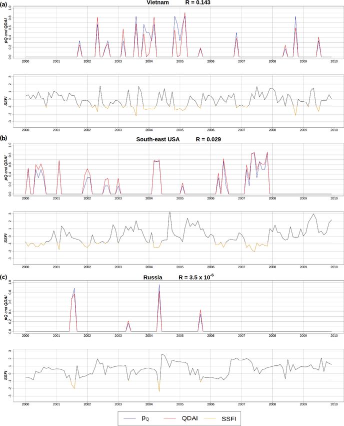
E. Popat and P. Döll: Soil moisture and streamflow deficit anomaly index                                                    1345

Figure 3. Frequency of occurrence [%] of different soil moisture drought classes during the period 1981–2010, as defined by SMDAI
(Table 2), and nc denotes grid cells which are not computed due to land cover.

4.6 km3 per month of the Rhine at Mainz (49.75◦ N, 8.25◦ E,        (dark blue line). This occurs because the decade shown in
right panels of Fig. 4).                                           Fig. 4 happens to be a very wet decade compared to the whole
   In the US grid cell, the difference between the                 reference period. Another reason is that more than 20 % of
mean monthly streamflow under the naturalized condi-               the years show zero streamflow in the calendar months Au-
tion (Qnat_mean ) and mean monthly simulated streamflow            gust and September such that pQ is zero in all 30 August and
(Qant_mean ) is high, especially in the growing period, due to     September months of the reference period; i.e., no drought is
large anthropogenic abstractions of streamflow water in the        indicated even in case of zero streamflow (see left panel of
drainage basin of the grid cell (observed in the topmost plot).    Fig. S7 in the Supplement). Due to the large deficit values,
While the observed (Qant_obs ) and simulated (Qant ) stream-       pQ is almost always smaller than dQ in this US grid cell.
flow shows a reasonable correlation, WaterGAP appears to              In the German grid cell (right panels in Fig. 4), the rel-
overestimate streamflow depletion by human water use in the        atively low anthropogenic surface water abstractions result
summers. Characterized by a high seasonality, anthropogenic        in almost identical values of Qnat_mean and Qant_mean (lines
surface water demand WUsw (dashed grey line in center plot)        overlap in the top plot), and total surface water demand is
and total surface water demand (i.e., WUsw + EFR_0.8, or-          very similar to EFR (lines overlap in the center plot). Non-
ange line in center plot) result in very high deficits dQ (green   zero dQ values (bottom plot) are mainly computed if Qant is
line of the bottom plot) during almost every summer. How-          lower than EFR, such as during the central European drought
ever, there are only a few months with drought as identified       of 2003. It is reasonable to consider this type of situation as
by the anomaly-based drought hazard pQ exceeding zero              a drought hazard as water supply companies would have to

https://doi.org/10.5194/nhess-21-1337-2021                                Nat. Hazards Earth Syst. Sci., 21, 1337–1354, 2021
1346                                              E. Popat and P. Döll: Soil moisture and streamflow deficit anomaly index

Figure 4. Streamflow drought hazard: example of a time series (2000–2010) of monthly surface water demand, surface water supply and
mean seasonality of surface water supply, as well as dQ , pQ and QDAI (e, f) for a cell in the USA (a, c, e) and Germany (b, d, f).

stop any surface water abstraction if they wished to protect        fact that total surface water demand is dominated in many
the river ecosystem. Different from the US grid cell, droughts      grid cells by EFR, which is a fraction of Qnat . In the EFR-
are rather equally distributed over all decades of the refer-       dominated cells, the mean monthly Qant is very similar to
ence period in the German grid cell but the summers of 2003         the mean monthly Qnat , such that dQ is then approximately
and 2005 suffer from the most severe droughts of the refer-         the difference between mean monthly Qant and Qant ; this
ence period, in line with expected drier summer due of cli-         difference is also the basis for computing by pQ (Fig. 5d).
mate change. Even if taking into account EFR as 80 % of             QDAI is mostly less than pQ (Fig. 5e). The 2003 central Eu-
Qnat_mean (EFR0.8 ), the total surface water demand is so low       ropean drought hazard for the surface water supply for hu-
that in contrast to the US cell, dQ is always smaller than pQ .     mans (Fig. 5d) is, at least in many parts of Germany, less
   Assumptions about the magnitude of EFR have a strong             pronounced than the soil moisture drought hazard for vege-
impact on dQ and thus QDAI of all grid cells except those           tation (Fig. 2c). Figure 5c–e also indicate the grid cells with
with very high surface water abstractions such as the US            Qant = 0. If streamflow in a grid cell is zero in 20 % or more
cell. If the water demand of the ecosystem were assumed             of all August months (left panel of Fig. S7), pQ and thus
to be only 20 % of Qnat_mean (EFR_0.2) instead of 80 % of           QDAI are zero because the zero streamflow is not an anomaly
Qnat_mean , dQ decreases somewhat in the US cell but reduces        that occurs in less than 1 out of 5 years.
to zero during the whole reference period in the German cell           In contrast to SMDAI, the frequency of occurrence of no-
(Fig. S6 in the Supplement). Therefore, water suppliers in the      drought conditions according to QDAI (Fig. 6) is larger than
German grid cell would not suffer from any drought hazard           80 % in grid cells, particularly with large rivers and barely
(as indicated by QDAI) and would not have to decrease their         any human water use, such as the Amazon River in South
surface water abstractions even during a drought similar to         America, the Congo River in Africa and the Ob River in
the 2003 central European drought.                                  Russia (Fig. 6e), where the deficit is often zero. In addition,
   The global streamflow drought hazard maps for August             grid cells with intermittent flows also show a high percent-
2003 (Fig. 5) help to illustrate the global variations in QDAI      age of no-drought conditions, as for any calendar month with
as a function of its components pQ and dQ , which again de-         at least 6 months without streamflow pQ is always equal to
pends on the human surface water demand WUsw . Stream-              zero (Fig. S7). In these grid cells, no-drought conditions oc-
flow deficits are not restricted to areas with high mean an-        cur in the case of zero streamflow. This type of intermittent
nual WUsw during the period 1981–2010 (Fig. 5a) but can be          grid cell, where Qant = 0 for at least 20 % of the months of
greater than 75 % in regions such as South Africa were Qant         any calendar month is marked separately in Fig. 6c–e. Ex-
is low (Fig. 5b). Different from soil moisture drought, pQ          treme streamflow drought hazard for human water supply
and dQ are strongly correlated (Fig. 5c). This is due to the        (Fig. 6d) occurs most often in regions with high streamflow

Nat. Hazards Earth Syst. Sci., 21, 1337–1354, 2021                                 https://doi.org/10.5194/nhess-21-1337-2021
E. Popat and P. Döll: Soil moisture and streamflow deficit anomaly index 1347
Figure 5. Global maps of mean annual WUsw , dQ , pQ , QDAI and the difference between QDAI and pQ for August 2003. Blue points in
(b) represent the location of the German and US grid cells from Fig. 4. Grid cells with Qant = 0 are indicated; nc: QDAI is not computed
due to land cover.
deficits (compare Fig. 5b), such as South Africa and parts of (Fig. 7a), psoil_Smax2 (Fig. 7c) and SMDAI_Smax2 (Fig. 7e)
southeastern Australia, i.e., regions with low streamflow and for August 2003 and the change in each parameter with re-
relatively high surface water abstractions, mainly for irriga- spect to the standard WaterGAP output, i.e., the difference
tion (Fig. 5a). Regions with low water human surface water between parameters computed using Smax2 and Smax (Fig. 7b,
abstractions such as northern Canada and the Amazon and d and f). With doubled Smax , mean monthly soil moisture in-
Congo basins show an exceptionally high occurrence of mild creases, too. In most grid cells, the soil moisture deficit in-
drought hazards (Fig. 6a). creases compared to standard Smax (Fig. 7b). Differences are
mostly small except for scattered grid cells in which the soil
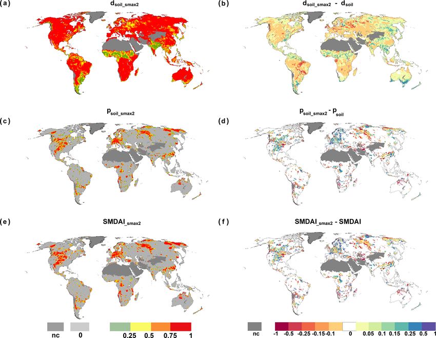
3.3 Sensitivity of SMDAI to the Smax values assumed in moisture deficit decreases by more than 50 percentage points.
WaterGAP Such cells are also found in central Europe where, under the
heavy drought conditions of August 2003, computed deficits
Smax is one of the key components for computing SMDAI. dQ are generally smaller in the case of doubled Smax ; in this
WaterGAP calibration and validation studies have indicated region, psoil increases in the case of doubled Smax (Fig. 7d).
that Smax may be underestimated in WaterGAP by a fac- Globally, psoil increases or decreases in some grid cells by
tor of 2 or more (Hosseini-Moghari et al., 2020). In order more than 50 percentage points. Equally, for SMDAI, the
to understand the sensitivity of SMDAI to changes in Smax , sensitivity to doubled Smax is low for most grid cells but can
we ran a version of WaterGAP in which Smax was dou- be greater for a few (Fig. 7e).
bled (Smax2 ). Figure 7 presents global maps of dsoil_Smax2
https://doi.org/10.5194/nhess-21-1337-2021 Nat. Hazards Earth Syst. Sci., 21, 1337–1354, 20211348 E. Popat and P. Döll: Soil moisture and streamflow deficit anomaly index
Figure 6. Frequency of occurrence [%] of different streamflow drought classes during the period 1981–2010 as defined by QDAI (Table 2).
Grid cells where for any calendar month there are at least 6 months with Qant = 0 are indicated as int, and grid cells which are not computed
due to land cover are indicated as nc.
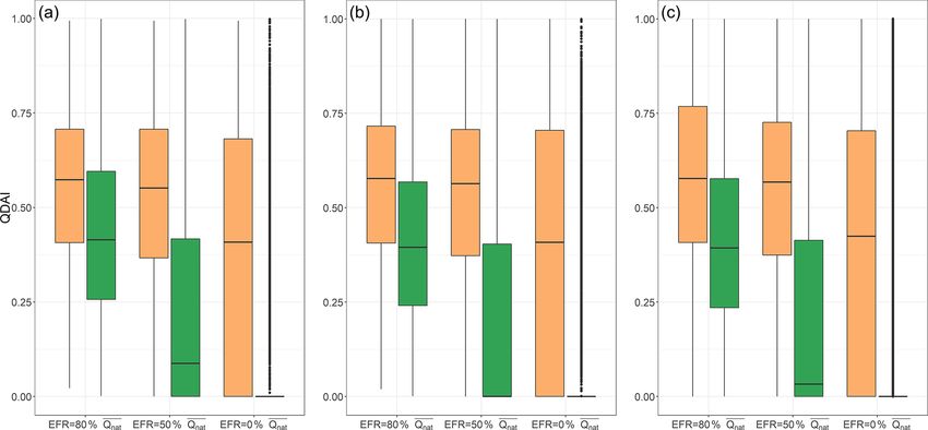
3.4 Sensitivity of QDAI to different assumptions about the river can be abstracted, they will very rarely be unable
EFR to satisfy their demand. In humid grid cells, QDAI increases
strongly with the selected EFR, which means that with in-
The streamflow drought hazard for water supply indicated creasing consideration of the water requirements of the river
by QDAI depends on how EFR is defined. In Fig. 8, we com- ecosystems, drought hazards to the water supply increase;
pare the global distribution of QDAI values among the 57 043 i.e., there are more situations where water abstractions would
0.5◦ grid cells, assuming that either 80 % or 50 % of mean have to be reduced to keep enough water in the river for the
monthly natural streamflow is required to remain in the river ecosystems to thrive. In (semi)arid regions, QDAI is already
for the well-being of the river ecosystem, or that there is no very high, even without acknowledging any water require-
EFR at all that needs to be considered when the decisions ment of the river ecosystem. This is due to an often high
about river water abstractions are made. We distinguish be- surface water demand compared to naturalized streamflow,
tween humid and (semi)arid grid cells (Fig. S8 in the Supple- in particular as crop production requires irrigation. Like in
ment) and consider the two months of August and December humid regions, QDAI increases with increasing EFR. The
2003 as well as all 360 months of the reference period. The slightly higher median QDAI values in August 2003 than
QDAI distributions are very similar for all three time periods. in December 2003 reflect the larger amount of humid grid
The boxplots show that a drought hazard in humid areas is cells in the Northern Hemisphere. Figure 8 shows that wa-
only identified if the existence of an EFR is acknowledged. ter suppliers in (semi)arid and arid regions suffer much more
If water suppliers in humid areas assume that all water in strongly from drought hazards than water suppliers in hu-
Nat. Hazards Earth Syst. Sci., 21, 1337–1354, 2021 https://doi.org/10.5194/nhess-21-1337-2021E. Popat and P. Döll: Soil moisture and streamflow deficit anomaly index 1349
Figure 7. Spatial representation of dsoil , psoil and SMDAI computed with Smax2 is presented in (a, c, e), and in (b, d, f) are the differences
in these dsoil , psoil and SMDAI compared to the results computed with the standard version of WaterGAP for August 2003. Grid cells which
are not computed due to land cover are denoted as nc.
mid areas due to the much higher ratio of water demand to have almost equal QDAI values for all three EFR alterna-
streamflow. tives.
Further differences between QDAI values computed for an
alternative EFR are explored for two widely known drought 3.5 Comparing QDAI to the standardized streamflow
events, the South Asian drought of 2009 (Neena et al., 2011) index (SSFI)
and the North American drought of 2002 (Seager, 2007). Fig-
ure 9 presents the spatial extent of both the droughts detected Like pQ , SSFI (see Sect. 2.6) assumes biota and humans are
by QDAI at a continental scale (left panels of Fig. 9) for Au- accustomed to the seasonal and interannual variability of the
gust 2009 and March 2002. Time series plots (right panels of streamflow. In order to quantify the added value of QDAI,
Fig. 9) for an Indian grid cell (24.75◦ N, 75.75◦ E, top panel), we compared QDAI values to SSFI values computed with
as well as another for a US grid cell (44.25◦ N, −110.75◦ E, a 1-month timescale. The anomaly of streamflow in SSFI
bottom panel), provide a better understanding of the sensi- was computed in the same manner as for pQ , by fitting the
tivity of QDAI to EFR. As expected, QDAI values calculated gamma cumulative distribution function for monthly Qant . It
with EFR = 0 (green) are lower and drought periods shorter was then transformed into a Gaussian distribution by calcu-
than if it is assumed that water needs to remain in the river for lating the mean and standard deviation, as well as using the
the well-being of the ecosystems. Interestingly, short but se- approximate conversion provided by Abramowitz and Ste-
vere droughts in the Indian grid cell in 2002, 2006 and 2010 gun (1965); this is also used by Kumar et al. (2009). Fig-
ure 10 shows three grid cells characterized by rather differ-
https://doi.org/10.5194/nhess-21-1337-2021 Nat. Hazards Earth Syst. Sci., 21, 1337–1354, 20211350 E. Popat and P. Döll: Soil moisture and streamflow deficit anomaly index Figure 8. Global distribution of QDAI in August 2003 (left) and December 2003 (middle) and for all 360 months of the reference period (right), computed with alternative assumptions about EFR for grid cells with humid and (semi)arid conditions. Grid cells where all three EFR assumptions result in QDAI = 0 are not included. Figure 9. Continental maps of QDAI for Asia and North America for August 2009 and March 2002, respectively (a, c), with blue points showing the locations of the Indian and US grid cells. Time series of different QDAI with alternative EFR for the Indian grid cell for 2001–2010 (b) and the US grid cell for 1998–2007 (d). Grid cells which are not computed due to land cover are denoted as nc. ent values of the ratio R of long-term average annual WUsw QDAI is based additionally on estimates of the grid cell’s to long-term average annual Qant : high (Vietnam, 10.75◦ N, specific human surface water demand and assumptions on 107.25◦ E in Fig. 10a), moderate (southeast USA, 31.75◦ N, EFR. A comparison of SSFI and QDAI is, therefore, essen- −84.75◦ E in Fig. 10b) and low (Russia, 63.75◦ N, 136.75◦ E tially a comparison of pQ and QDAI. If R is very small, such in Fig. 10c). as in the case of the Russian grid cell, with R = 3.5 × 10⁻⁶ As expected, pQ and SSFI show an equivalent behavior in (Fig. 10c), QDAI is very similar to pQ , while dQ is very all grid cells as they are based on the same streamflow data, similar to EFR, being 80 % of the mean monthly Qnat (see do not use any additional information and can be mathemati- explanation in Sect. 3.2). For the Vietnamese grid cell with a cally transformed from one to the other (Table 1). In contrast, high R value of 0.143, QDAI does not interpret the anoma- Nat. Hazards Earth Syst. Sci., 21, 1337–1354, 2021 https://doi.org/10.5194/nhess-21-1337-2021
E. Popat and P. Döll: Soil moisture and streamflow deficit anomaly index                                                              1351

Figure 10. Time series of QDAI and SSFI for grid cells with different ratios of surface water abstractions to streamflow R in three regions:
(a) Vietnam (10.75◦ N, 107.25◦ E), (b) southeast USA (31.75◦ N, −84.75◦ E) and (c) Russia (63.75◦ N, 136.75◦ E). SSFI is shown in red if
it is below −0.84 standard deviations, corresponding to a 5-year return period and a p of zero (Table 1).

https://doi.org/10.5194/nhess-21-1337-2021                                      Nat. Hazards Earth Syst. Sci., 21, 1337–1354, 2021
1352                                              E. Popat and P. Döll: Soil moisture and streamflow deficit anomaly index

lously low streamflow values in December 2003 and Decem-          type or income levels. In regional or global drought risk stud-
ber 2005 as a drought hazard due to the low human water           ies, the inclusion of grid-scale values of QDAI and SM-
demand for surface water in December. Globally averaged,          DAI would be beneficial as both indices contain spatially
the fraction of months under drought during 1981–2010 is          highly resolved information on vulnerability, while most
16.0 % according to QDAI and 19.1 % according to SSFI.            other vulnerability indicators represent spatial averages of
This reflects that QDAI only identifies a drought condition       much larger spatial units such as countries.
if there is, in addition to the anomalously low flow, a water
deficit.
                                                                  Data availability. WaterGAP 2.2d model output data used in this
                                                                  study are available at https://doi.org/10.1594/PANGAEA.918447
4   Conclusions                                                   (Müller Schmied et al., 2020). The outputs from this study are avail-
                                                                  able at https://doi.org/10.6084/m9.figshare.14213852 (Popat and
                                                                  Döll, 2021).
In this paper, we presented two drought hazard indices that
combine the drought deficit and anomaly characteristics: one
for soil moisture drought (SMDAI) and the other for stream-
                                                                  Supplement. The supplement related to this article is available on-
flow drought (QDAI). With SMDAI, which describes the
                                                                  line at: https://doi.org/10.5194/nhess-21-1337-2021-supplement.
drought hazard for vegetation, we achieved the simplifica-
tion of the deficit-anomaly-based Drought Severity Index in-
troduced by Cammalleri et al. (2016). We transferred the          Author contributions. This paper was conceptualized by PD with
DSI concept to streamflow drought, creating an indicator that     input from EP. EP performed the data analysis and visualization.
specifically quantifies the hazard that drought poses for water   The original draft was written by EP and revised by PD.
supply from rivers. To our knowledge, QDAI is the first ever
streamflow drought indicator that combines the anomaly and
deficit aspects of streamflow drought.                            Competing interests. The authors declare that they have no conflict
   The concept of SMDAI and QDAI was tested at the global         of interest.
scale by using simulated data from the latest version of the
global water resources and using the model WaterGAP. Con-
versely the reliability of the computed SMDAI and QDAI            Special issue statement. This article is part of the special issue “Re-
values strongly depends on the quality of the model out-          cent advances in drought and water scarcity monitoring, modelling,
put. The indicators themselves have been proven to provide        and forecasting (EGU2019, session HS4.1.1/NH1.31)”. It is a re-
meaningful quantitative estimates of drought hazard that de-      sult of the European Geosciences Union General Assembly 2019,
                                                                  Vienna, Austria, 7–12 April 2019.
pend not only on the unusualness of the situation but also
on the concurrent deficit of available water compared to
demand. We found that the values of the combined deficit
                                                                  Acknowledgements. We thank Hannes Müller Schmied for input
anomaly drought indices are often broadly similar to purely       and guidance on setting up the WaterGAP variant with doubled
anomaly-based indices and share with them the difficulty of       Smax (Sect. 4.1.1) and Thedini Asali Peiris for constructive criti-
dealing with intermittent streamflow regimes. However, they       cism of the manuscript. Also, we acknowledge funding from the
do provide more differentiated spatial and temporal patterns      German Federal Ministry of Education and Research (BMBF) for
and help to distinguish the degree and nature of the drought      the “Globe Drought” project through its funding measure Global
hazard. QDAI can serve as a tool for informing water sup-         Resource Water (GRoW) (grant no. 02WGR1457B).
pliers and other stakeholders about the joint drought hazard
for water supply for both humans and the river ecosystem,
while stakeholders may adapt the EFR applied for comput-          Financial support. This research has been supported by the
ing QDAI in accordance with their valuation of ecosystem          German Federal Ministry of Education and Research (BMBF)
health. Like all hydrological drought indicators that reflect     (grant no. 02WGR1457B).
streamflow anomaly, QDAI needs to be interpreted carefully
                                                                  This open-access publication was funded
in case of highly intermittent streamflow regimes.
                                                                  by the Goethe University Frankfurt.
   The term “drought hazard” can be defined as the source of
a potential adverse effect of an unusual lack of water on hu-
mans or ecosystems. In this sense, SMDAI and QDAI are
                                                                  Review statement. This paper was edited by Carmelo Cammalleri
drought hazard indicators, even if they include some ele-         and reviewed by two anonymous referees.
ments of vulnerability to drought. Both SMDAI and QDAI
are well applicable in drought risk studies. In local drought
risk studies, additional indicators of ecological or societal
vulnerability should be added, for example, vegetation/crop

Nat. Hazards Earth Syst. Sci., 21, 1337–1354, 2021                                 https://doi.org/10.5194/nhess-21-1337-2021
You can also read