Towards a compound-event-oriented climate model evaluation: a decomposition of the underlying biases in multivariate fire and heat stress hazards ...
←
→
Page content transcription
If your browser does not render page correctly, please read the page content below
Nat. Hazards Earth Syst. Sci., 21, 1867–1885, 2021
https://doi.org/10.5194/nhess-21-1867-2021
© Author(s) 2021. This work is distributed under
the Creative Commons Attribution 4.0 License.

Towards a compound-event-oriented climate model
evaluation: a decomposition of the underlying biases
in multivariate fire and heat stress hazards
Roberto Villalobos-Herrera1,2 , Emanuele Bevacqua3,4 , Andreia F. S. Ribeiro5,6 , Graeme Auld7 , Laura Crocetti8,9 ,
Bilyana Mircheva10 , Minh Ha11 , Jakob Zscheischler4,12,13 , and Carlo De Michele14
1 School  of Engineering, Newcastle University, Newcastle upon Tyne, NE2 1HA, UK
2 Escuela  de Ingeniería Civil, Universidad de Costa Rica, Montes de Oca, San José 1150-2060, Costa Rica
3 Department of Meteorology, University of Reading, Reading, UK
4 Department of Computational Hydrosystems, Helmholtz Centre for Environmental Research – UFZ, Leipzig, Germany
5 Instituto Dom Luiz (IDL), Faculdade de Ciências, Universidade de Lisboa, 1749-016 Lisbon, Portugal
6 Institute for Atmospheric and Climate Science, ETH Zurich, Universitätstrasse 16, Zurich 8092, Switzerland
7 School of Mathematics, The University of Edinburgh, Edinburgh, UK
8 Department of Geodesy and Geoinformation, TU Wien, Vienna, Austria
9 Institute of Geodesy and Photogrammetry, ETH Zurich, Zurich, Switzerland
10 Department of Meteorology and Geophysics, Sofia University “St. Kliment Ohridski”, Sofia, Bulgaria
11 Laboratoire Atmosphères, Milieux, Observations Spatiales (LATMOS), Sorbonne Université, Paris and Guyancourt, France
12 Climate and Environmental Physics, University of Bern, Bern, Switzerland
13 Oeschger Centre for Climate Change Research, University of Bern, Bern, Switzerland
14 Department of Civil and Environmental Engineering, Politecnico di Milano, Milan, Italy

Correspondence: Roberto Villalobos Herrera (r.villalobos-herrera2@newcastle.ac.uk)
and Emanuele Bevacqua (emanuele.bevacqua@ufz.de)

Received: 18 November 2020 – Discussion started: 23 November 2020
Revised: 23 March 2021 – Accepted: 6 May 2021 – Published: 17 June 2021

Abstract. Climate models’ outputs are affected by biases that     ity. The spatial pattern of the hazard indicators is well repre-
need to be detected and adjusted to model climate impacts.        sented by climate models. However, substantial biases exist
Many climate hazards and climate-related impacts are asso-        in the representation of extreme conditions, especially in the
ciated with the interaction between multiple drivers, i.e. by     CBI (spatial average of absolute bias: 21 ◦ C) due to the bi-
compound events. So far climate model biases are typically        ases driven by relative humidity (20 ◦ C). Biases in WBGT
assessed based on the hazard of interest, and it is unclear       (1.1 ◦ C) are small compared to the biases driven by tem-
how much a potential bias in the dependence of the hazard         perature (1.9 ◦ C) and relative humidity (1.4 ◦ C), as the two
drivers contributes to the overall bias and how the biases in     biases compensate for each other. In many regions, also bi-
the drivers interact. Here, based on copula theory, we develop    ases related to the statistical dependence (0.85 ◦ C) are im-
a multivariate bias-assessment framework, which allows for        portant for WBGT, which indicates that well-designed phys-
disentangling the biases in hazard indicators in terms of the     ically based multivariate bias adjustment procedures should
underlying univariate drivers and their statistical dependence.   be considered for hazards and impacts that depend on multi-
Based on this framework, we dissect biases in fire and heat       ple drivers. The proposed compound-event-oriented evalua-
stress hazards in a suite of global climate models by con-        tion of climate model biases is easily applicable to other haz-
sidering two simplified hazard indicators: the wet-bulb globe     ard types. Furthermore, it can contribute to improved present
temperature (WBGT) and the Chandler burning index (CBI).          and future risk assessments through increasing our under-
Both indices solely rely on temperature and relative humid-

Published by Copernicus Publications on behalf of the European Geosciences Union.
1868                          R. Villalobos-Herrera et al.: Towards a compound-event-oriented climate model evaluation

standing of the biases’ sources in the simulation of climate       sessment both in the present and future climate. However,
impacts.                                                           studies evaluating the climate model multivariate representa-
                                                                   tion of hazard indicator are still rare (Bevacqua et al., 2019;
                                                                   Zscheischler et al., 2021), and little is known on the effects
                                                                   of those biases on multivariate hazards (Fischer and Knutti,
1   Introduction                                                   2013; Zscheischler et al., 2018).
                                                                      In this study we propose a copula-based multivariate bias-
Understanding and assessing the risk of high-impact events         assessment framework, which allows for decomposing the
induced by the combination of multiple climate drivers             sources of bias in hazard indicators. We employ global cli-
and/or hazards, referred to as compound events, is chal-           mate model outputs from the fifth phase of the Coupled
lenging (e.g. Bevacqua et al., 2017; Manning et al., 2018;         Model Intercomparison Project (CMIP5) and consider two
Zscheischler et al., 2020). One of the reasons is that many        simplified hazard indices, the Chandler burning index (CBI)
high-impact events are caused by multiple variables that may       for fire hazard and the wet-bulb globe temperature (WBGT)
not be extreme themselves, but their combination leads to          index for heat stress, both driven solely by temperature and
an extreme impact (Zscheischler et al., 2018). For exam-           relative humidity. Figure 1 illustrates the main rationale of
ple, the risks associated with combined high temperature and       the multivariate bias-assessment framework. Both hazard in-
high/low relative humidity such as heat stress and fires can       dices, CBI and WBGT, are influenced by the bivariate distri-
manifest in heat-related human fatalities (Raymond et al.,         bution of temperature and relative humidity (Fig. 1c). Based
2020) and fire-induced tree mortality (Brando et al., 2014)        on copula theory, such a bivariate distribution can be decom-
even if the two contributing variables are not necessarily ex-     posed in terms of the marginal distributions of temperature
treme in a statistical sense. In the future, combinations of       and relative humidity (Fig. 1a and d), as well as their statis-
climate variables leading to disproportionate impacts will be      tical dependence (Fig. 1b). Hence, such a copula-based de-
affected by global warming, and reliable risk assessments are      composition allows for understanding the biases in the haz-
required (Fischer and Knutti, 2013; Russo et al., 2017; Schär,     ard estimates in terms of the contribution from the marginal
2016; Raymond et al., 2020; Jézéquel et al., 2020; Zscheis-        distributions individually (Fig. 1a and d; see difference be-
chler et al., 2020). Therefore, a better understanding of how      tween grey and black lines) and from their statistical depen-
climate models represent the joint behaviour of variables be-      dence (Fig. 1b) (Vezzoli et al. 2017; Bevacqua et al., 2019).
hind compound events, such as temperature and relative hu-         We present a methodology to quantify the role played by
midity, is crucial to correctly quantify their associated haz-     the biases in temperature, relative humidity, and their depen-
ards today and in the future (Zscheischler et al., 2018).          dence in the final bias in the fire and heat stress indices as
   Typically, the raw climate model data contain biases,           simulated by climate models.
which lead to biased estimates of climate risks (Maraun et al.,
2017). Evaluating, i.e. assessing and understanding, such bi-
ases is a crucial step towards impact modelling and thus as-       2     Data
sessment of future climate risks. Climate model evaluation
is very often univariate; i.e. it does not take into account the   2.1    Pre-processing
multivariate nature of many hazards that are driven by the
interplay of multiple contributing variables (Vezzoli et al.,      We employ 6-hourly data of 2 m air temperature (T )
2017; Zscheischler et al., 2018, 2019; Francois et al., 2020).     and relative humidity (RH) during the period 1979–2005
However, evaluating the model representation of the individ-       from ERA-Interim reanalysis (Berrisford et al., 2011;
ual contributing variables individually, and hence disregard-      Dee et al. 2011) and 12 models from the CMIP5 mul-
ing both the biases in the dependence between the contribut-       timodel ensemble (Taylor et al., 2012): ACCESS1-0,
ing variables and how the biases in the drivers combine to         ACCESS1-3, BCC-CSM1.1-m, BNU-ESM, CNRM-CM5,
influence the hazard, cannot provide direct information re-        GFDL-ESM2G, GFDL-ESM2M, INM-CM4, IPSL-CM5A-
garding the biases in the resulting hazard indicator. Further-     LR, NorESM1-M, GFDL-CM3, and IPSL-CM5A-MR; leap
more, evaluating the hazard indicator only, e.g. heat stress       days were removed. To allow for an intermodel comparison,
regardless of the contributing variables temperature and rela-     data were bilinearly interpolated to a 2.5◦ by 2.5◦ regular
tive humidity, may hide compensating biases in the contribut-      latitude–longitude grid. All oceanic grid cells as well as those
ing variables, even if the hazard indicator appears to be well     beneath 60◦ S were removed from all analyses, given that ar-
represented. An evaluation of climate models that considers        guably no heat stress and fire risk exists in these areas.
the underlying multivariate nature of the hazards can provide         Following Zscheischler et al. (2019), we restrict our analy-
a better physical understanding of the relevant model skills.      sis to the hottest calendar month of the year, which is selected
In turn, a better understanding of model skills can serve as       based on the climatology of ERA-Interim data at each grid
a basis for better adjustment of the biases and/or selection       point. This choice was made because arguably heat stress and
of best-performing models, which are crucial for hazard as-        fire hazards tend to be more frequent during the warmest pe-

Nat. Hazards Earth Syst. Sci., 21, 1867–1885, 2021                                https://doi.org/10.5194/nhess-21-1867-2021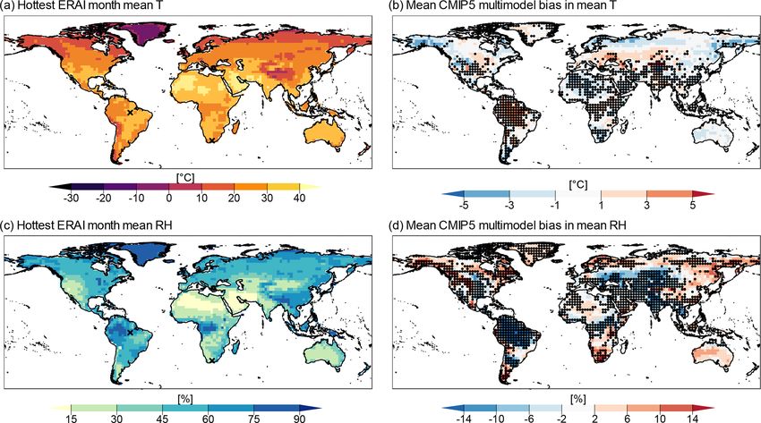
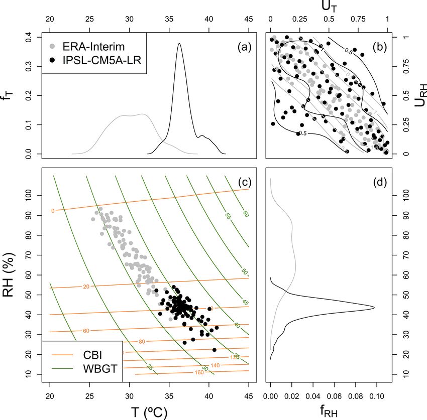
R. Villalobos-Herrera et al.: Towards a compound-event-oriented climate model evaluation                                                1869

Figure 1. Copula-based conceptual framework employed in this study to evaluate biases in CBI and WBGT indices. The framework is
illustrated for a representative location in Brazil (Amazonia, 5◦ S and 56.5◦ W; indicated via X markers in the next figures). Panel (c) shows
the bivariate distribution of T and RH based on ERA-Interim (grey) and IPSL-CM5A-LR data (black) during 1979–2005. Isolines indicate
equal levels of CBI (orange) and WBGT (green). The decomposition of biases from the marginals (a, d) and the copula (b) are illustrated as
the discrepancies between the black (IPSL-CM5A-LR model) and grey features (ERA-Interim).

riod of the year, and it avoids dealing with seasonality; how-           for which the autocorrelation was non-significant at the 95 %
ever we note that this assumes that CMIP5 models correctly               confidence level was determined. Finally, the maximum of
reproduce the seasonality observed in ERA-Interim. Finally,              all the minimum lags was selected, resulting in N = 9 d. The
for each model and location, we consider the T and RH val-               time series for all models and locations are sampled with the
ues at the daily 6-hourly time steps corresponding to the daily          frequency of N. This is done N times using different start
maximum temperature within the hottest month. The above                  epochs, where the first sampled time series starts with time
results in a time series for each location and model, with daily         epoch one, the second sampled time series with time epoch
values of the pair (T , RH).                                             two, and so on up to nine. The decorrelated time series of T
   The resulting time series data are autocorrelated, which              and RH will henceforth be simply referred to as samples in
can compromise the interpretation of the statistical tests that          the following sections.
we apply in the analysis (Yue et al., 2002; Dale and Fortin,                In the Appendix, Fig. A1 illustrates, for a representative
2009). Therefore, we carry out the analysis on the decor-                location in Brazil, one of the nine resulting samples of T and
related time series, which are obtained from the original                RH for ERA-Interim and for a selection of CMIP5 models.
through subsampling every N = 9 d, where N is the lag re-                The figure also shows how the bivariate interaction of these
quired to remove the autocorrelation in T and RH time se-                variables drives the fire and heat stress indices (coloured iso-
ries data everywhere (at 95 % confidence level). The value of            lines) introduced in the next section.
N was determined as follows: for all individual grid points
and years in ERA-Interim and the CMIP5 models, the auto-
correlation function was calculated; then, the minimum lag

https://doi.org/10.5194/nhess-21-1867-2021                                       Nat. Hazards Earth Syst. Sci., 21, 1867–1885, 2021
1870                                R. Villalobos-Herrera et al.: Towards a compound-event-oriented climate model evaluation

2.2     Fire hazard and heat stress indices                                  how bias in each of these components contributes to the bias
                                                                             in CBI and WBGT.
We quantify fire and heat stress hazards based on two indices,                  A copula is a function that completely characterizes the
i.e. CBI and WBGT, respectively. While more advanced and                     dependence structure between random variables, in our case
sophisticated indices exist for both of these hazards (e.g. Van              T and RH. Sklar’s theorem (Sklar, 1959) is a fundamental
Wagner, 1987; Fiala et al., 2011), here we employ these two                  result in copula theory, which states that the joint distribu-
simplified indices. Our aim is to provide a methodological                   tion of the random variables is determined by the marginal
framework for a compound-event-oriented evaluation of haz-                   distributions and their copula. Mathematically, in our bivari-
ard indicators. Hence, employing simplified indices allows                   ate case, given the two variables T and RH, with marginal
for the development of a test case of the methodological                     cumulative distribution functions (CDFs) FT and FRH , and
framework. We do not aim at providing an accurate assess-                    marginal probability density functions (PDFs) fT and fRH ,
ment of the hazard; nevertheless, our results will provide in-               following Sklar’s theorem, the joint PDF fT,RH can be de-
dications that can serve as a basis for follow-up studies of                 composed as
more complex fire and heat stress hazards.
   The CBI index was employed, for example, for studying                     fT,RH (T , RH) = fT (T ) · fRH (RH) · c(UT , URH ),         (3)
fire risk in the United States (McCutchan and Main, 1989)
and globally (Roads et al., 2008). The index is based on air                 where URH = FRH (RH), UT = FT (T ) (note that U indicates
T (◦ C) and RH (%):                                                          that both URH and UT are uniformly distributed by construc-
                                                                             tion on the domain [0,1]), and c is the copula density, which
         ((110 − 1.73 · RH) − 0.54 · (10.20 − T )) · 1.24 × 10−0.0142·RH     describes the dependence of the joint distribution fT,RH inde-
CBI =                                                                    .
                                       60                                    pendently from the marginal distributions fT and fRH . Note
                                                                       (1)   that Eq. (3) naturally extends to the case of an arbitrary
                                                                             number of random variables (Bevacqua et al., 2017); how-
   The “simplified WBGT” (from now on WBGT for the sake
                                                                             ever here we focus on the bivariate case. Copulas allow for
of brevity) index was developed by the American College
                                                                             great flexibility in modelling complex dependence structures
of Sports Medicine (ACSM, 1984) as an indicator of heat
                                                                             between several variables, and there are a huge variety of
stress for average daytime conditions outdoors. The index is
                                                                             parametric copula families available for statistical modelling
defined as
                                                                             purposes (Nelsen, 2006; Salvadori and De Michele, 2007;
                                                                             Salvadori et al., 2007; Durante and Sempi, 2015; Bevacqua
WBGT = 0.56T + 0.393e + 3.94,                                          (2)
                                                                             et al., 2020a). However, note that following the methodolo-
where e = (RH/100) · 6.105e(17.27T /(237.7+T )) is water                     gies developed by Rémillard and Scaillet (2009) and Vezzoli
vapour pressure (expressed in hPa), which depends on air                     et al. (2017), here we will consider a non-parametric frame-
temperature and relative humidity. More details on the def-                  work; i.e. we will consider empirical, rather than paramet-
initions of the CBI and WBGT are available at McCutchan                      ric, distributions within our testing procedures. This choice
and Main (1989) and ACSM (1984).                                             avoids unnecessary parametric-based assumptions on the dis-
                                                                             tributions that could bias the results about both univariate and
                                                                             multivariate features.
3     Methods                                                                   A characteristic of copulas is the invariance property (Sal-
                                                                             vadori et al. 2007, proposition 3.2); i.e. if g1 and g2 are
This section presents the conceptual framework and a bias                    monotonic (increasing) functions, then the transformed vari-
decomposition methodology used to analyse the multivariate                   ables g1 (T ) and g2 (RH) have the same copula as T and
indices described above. We then present an overview of the                  RH. This property is crucial to the methodology described
data processing before detailing the conventional statistical                in the following section, where the monotonic functions are
tests we have incorporated into our test suite.                              the marginal CDFs of T and RH (or their inverses).

3.1     Copula-based conceptual framework                                    3.2   Contribution of the bias in the drivers to the bias of
                                                                                   CBI and WBGT
As both CBI and WBGT are functions of T and RH, it fol-
lows that their distributions are determined by the joint dis-               We assess how biases in each of the marginal distributions of
tribution of T and RH. Copula theory provides us with a nat-                 Tmod and RHmod , and Cmod (the copula of Tmod and RHmod ),
ural way to decompose the joint distribution of T and RH in                  contribute to the bias in the representation of the extreme val-
terms of the marginal distributions of T and RH (the distribu-               ues of CBI and WBGT (extremes are defined based on 95th
tions of the individual variables considered in isolation) and               percentiles (Q95)). This is achieved based on a methodology
a term, known as the copula, that describes the dependence                   originally introduced by Bevacqua et al. (2019) to attribute
between T and RH (Fig. 1). This allows us to understand                      changes in compound flooding to its underlying drivers (and

Nat. Hazards Earth Syst. Sci., 21, 1867–1885, 2021                                          https://doi.org/10.5194/nhess-21-1867-2021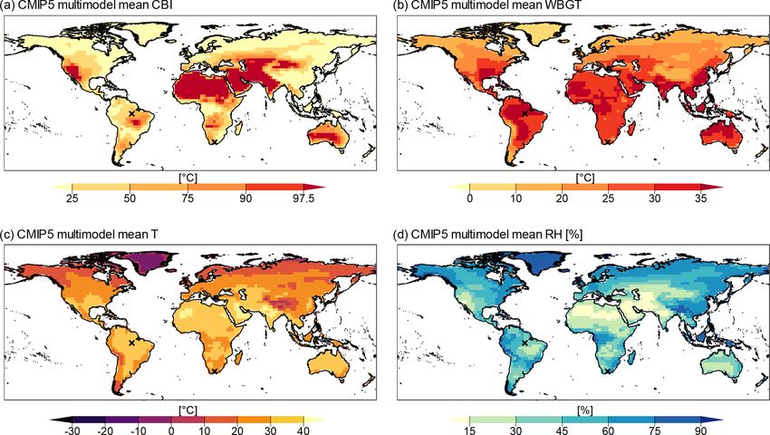
R. Villalobos-Herrera et al.: Towards a compound-event-oriented climate model evaluation                                           1871

employed by for example Manning et al., 2019, and Bevac-               ing, we use the conservative Bonferroni correction method,
qua et al., 2020b).                                                    which penalizes the significance level α using the number of
   We carried out three experiments. In experiment i, we ob-           repeated tests m = 9, so that the individual hypothesis tests
tained, via a data transformation, a bivariate pair (Ti , RHi )        are evaluated at an α/m significance level (Jafari and Ansari-
with copula Ci , where one component of the three underly-             Pour, 2019). A 5 % significance level is used, after which the
ing distributions (Ti , RHi , Ci ) is the same as that of a given      Bonferroni correction was adjusted to 0.0056 for use in each
CMIP5 model, and the other two components are the same as              individual hypothesis test. All of our analysis was carried out
ERA-Interim. We then perform the quantile tests described              in R (R Core Team, 2019), and the functions used for each
in Sect. 3.3.3 for CBI (or WBGT) using values based on (Ti ,           test are detailed in their corresponding section below.
RHi ) and (Terai , RHerai ). The specific experiments carried out         Graphically, the statistical test results are presented as a
are described below.                                                   percentage of all 108 CMIP5 model samples (9 samples
   Experiment (a) assesses the bias contribution of Tmod .             times 12 models) where the null hypothesis is rejected. The
From the variable Terai we calculated the uniformly dis-               percentage we consider is calculated at each grid cell, and
tributed transformed random variable UT,erai = FT,erai (Terai ).       stippling is added where the null hypothesis is rejected in at
From the variable Tmod we calculated the empirical CDF                 least 75 % (81/108) of all CMIP5 model samples.
                                                 −1
FT,mod , through which we defined Ta = FT,mod        (UT,erai ). The
variable Ta has the same distribution as Tmod , while the pair         3.3.1   Univariate evaluation of T , RH, CBI, and WBGT
(Ta , RHerai ) has the copula of ERA-Interim.
   Experiment (b) assesses the bias contribution of RHmod .            In order to understand how faithfully the marginal distribu-
This experiment follows the same structure as Experiment (a)           tions of T , RH, CBI, and WBGT from the ERA-Interim data
but with the roles of Terai and RHerai reversed, from which we         are represented in a given CMIP5 model, we perform the
get the pairs (Terai , RHb ).                                          two-sample Anderson–Darling (AD) test via the ad.test func-
   Experiment (c) assesses the bias contribution of Cmod .             tion of the kSamples R package (v1.2-9; Scholz and Zhu,
From the variables Tmod and RHmod we calculated the asso-              2019). This is a non-parametric procedure that considers the
ciated marginal empirical cumulative distributions (UT,mod ,           null hypothesis: “the two samples are from the same distri-
URH,mod ). From the variables Terai and RHerai , we defined            bution”.
the empirical CDFs FT,erai and FRH,erai , through which we
                  −1                              −1                   3.3.2   Dependence between T and RH
defined Tc = FT,erai   (UT,mod ) and RHc = FRH,erai     (URH,mod ).
The pair of variables (Tc , RHc ) have the same marginal distri-       A simple way to test how well the dependence between the
butions as the pair (Terai , RHerai ), but the copula of the model,    variables T and RH in ERA-Interim is represented in a given
i.e. Cmod , since (Tc , RHc ) was obtained from (Tmod , RHmod )        CMIP5 model is to compare the calculated values of some
by monotonic transformations of the margins.                           statistical measure of association. Here we use Kendall’s
                                                                       τ rank correlation. The cor.test function of the core stats
3.3   Description of the testing procedure                             R package was used to perform all τ calculations (R Core
                                                                       Team, 2019).
The full data processing procedure is shown in Fig. A2. We                To test whether the values of τ obtained from a given
began with the ERA-Interim and CMIP5 data and obtained                 model sample differ in a statistically significant way from the
T and RH samples (see Sect. 2.1). The CMIP5 samples were               corresponding ERA-Interim values, we begin by considering
then subject to the transformation procedure described in              the approximate 100(1 − α) % confidence interval (τL , τU )
Sect. 3.2.4. This results in five sets of T and RH data cor-           for τ associated with the point estimator τ̂ given by
responding to the ERA-Interim reference, the original model
sample, and the three experiments (a, b, and c) used to assess         τL = τ̂ − zα/2 σ̂, τU = τ̂ + zα/2 σ̂,                         (4)
the bias contributions of biases in CMIP5 model T , RH, and
their copula. At this stage, the CBI and WBGT indices are              where σ̂ 2 is an estimator of var(τ̂ ) and zα/2 is the quantile
calculated on all five sets.                                           of the standard normal distribution for α/2 (Hollander et al.,
   We execute univariate and multivariate non-parametric               2014). For our testing we calculate σ̂ 2 , τ̂ , and the confidence
statistical tests to evaluate the properties of CBI, WBGT, and         interval (τL , τU ) for each grid cell in all ERA-Interim sam-
their driver variables (i.e. T , RH, and their dependence) prior       ples, using a customized version of the kendall.ci function
to proceeding with our bias decomposition approach. Details            included in the NSM3 R package (v1.15, Schneider et al.,
for each of the tests are provided below, but, in general, we          2020). The CMIP5 model samples are then evaluated in two
follow a non-parametric approach similar to Vezzoli et al.             ways. Firstly, if the model sample value of τ lies within the
(2017). Each of the nine decorrelated ERA-Interim samples              confidence interval calculated for its corresponding ERA-
was independently tested on a cell-by-cell basis against a dif-        Interim sample, the model sample is judged to not signifi-
ferent CMIP5 model sample; therefore each statistical test is          cantly differ from ERA-Interim in terms of the rank corre-
repeated nine times per model. To adjust for multiple test-            lation between T and RH. Secondly, we calculated the zα/2

https://doi.org/10.5194/nhess-21-1867-2021                                     Nat. Hazards Earth Syst. Sci., 21, 1867–1885, 2021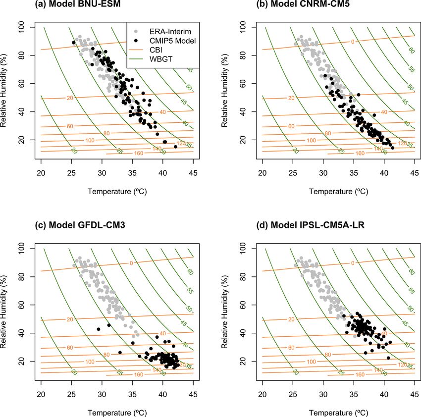
1872                          R. Villalobos-Herrera et al.: Towards a compound-event-oriented climate model evaluation

and hence the α or p value for each sample; these were tested     4     Results
for significance using the same Bonferroni-adjusted value
of 0.0056 used in the univariate testing. The results from        4.1     Univariate evaluation of T , RH, CBI, and WBGT
both testing methodologies are consistent with each other, we
present the ad hoc p-value test results in the main text, and     4.1.1    CBI and WBGT
the confidence interval tests are included in the Appendix.
   Note that different copulas may give rise to the same value    We began our analysis by visualizing the multimodel mean
of τ ; therefore we cannot conclude that a model that faith-      of the mean values of CBI and WBGT during the hottest
fully reproduces the ERA-Interim values of τ is accurately        months. According to reanalysis, the mean CBI is highest
representing the full dependence structure between T and          in regions with dry and warm weather during the hottest
RH. Therefore, we account for differences in the depen-           month, such as the Sahara, most of Australia, and the west-
dence structure by also carrying out hypothesis tests which       ern USA and Mexico (Fig. 2a). In contrast, CBI tends to be
are based on the full copula function. We perform the non-        low in humid and warm regions such as the Amazon and
parametric test of copula equality based on the Cramér–           Congo basins. We move to evaluating the CMIP5 model bi-
von Mises test statistic proposed by Remillard and Scaillet       ases in mean CBI, which appear large in magnitude (com-
(2009), used in Vezzoli et al. (2017) for testing the capabil-    pare Fig. 2b and a); most land masses are covered in dark red
ity of a climate–hydrology model to reproduce the depen-          or blue colours, indicating CMIP5 multimodel mean bias of
dence between temperature, precipitation, and discharge for       over 10 ◦ C from the ERA-Interim. In addition, AD test re-
the Po river basin in Italy, and recently employed by Zscheis-    sults show that 59 % of the global land mass has significant
chler and Fischer (2020) for evaluating the ability of climate    differences between ERA-Interim and CMIP5 distributions
models to represent the dependence between temperature and        of CBI in at least 75 % of model samples. Despite such biases
precipitation in Germany. The copula equality test has a null     in the representation of the mean CBI magnitude, the over-
hypothesis of H0 : Cerai = Cmod , where Cerai and Cmod are        all spatial patterns in mean CBI are well reproduced by the
the copulas of T and RH represented in ERA-Interim and a          models. In fact, the area-weighted pattern correlation (Pfahl
given model, respectively, with the alternative hypothesis be-    et al., 2017), from now on pattern correlation, between mod-
ing that these copulas differ. Unlike the AD test, which can      els and reanalysis of mean CBI is high for all CMIP5 mod-
evaluate CMIP5 model performance in reproducing a single          els, with a minimum value of 0.77 for the BCC-CSM1.1-m
marginal distribution, the copula equality test was specifi-      model (Fig. A3a shows the multimodel mean of mean CBI).
cally developed to test whether two empirical copulas are            In the reanalysis data, mean WBGT values over 30 ◦ C are
equal and thus evaluates the capacity of models to repro-         reached over most tropical land masses during each loca-
duce the full dependency structure between T and RH. We           tion’s hottest month, with lower values in higher latitudes
used the TwoCop function of the TwoCop R package (v1.0,           and the highest values near the Equator (Fig. 2c). For WBGT,
Remillard and Plante, 2012) to run the test.                      the pattern correlation between models and ERA-Interim is
                                                                  higher than for CBI, with a minimum value of 0.89 for the
3.3.3   Bias in the representation of extreme events of           BCC-CSM1.1-m model (Fig. A3b shows the multimodel
        CBI and WBGT                                              mean of mean WBGT). Mean multimodel bias in WBGT
                                                                  shows large parts of the continents are within the ± 0.5 ◦ C
To evaluate how well CMIP5 models simulate extreme val-           range relative to ERA-Interim. The AD test results indicate
ues of CBI and WBGT, we compare high quantiles (i.e. the          that the WBGT distributions in CMIP models are typically
95th percentile Q95) of these indices from each model with        better than those of CBI; only 35 % of grid cells fail our per-
those of ERA-Interim. To assess whether the observed differ-      formance criterion (Fig. 2d).
ences in the quantiles are statistically significant, we calcu-      Overall, CMIP5 models underperform in key regions as-
late the 95 % confidence intervals for the Q95 of CBI and         sociated with high fire and heat stress hazards. CBI’s dis-
WBGT at each location for ERA-Interim based on 1000               tribution is not well represented by most CMIP5 models in
bootstrap samples. Like our evaluation of Kendall’s τ , if the    regions characterized by high fire hazard levels such as the
model index lies outside the confidence interval, we consider     western USA and the Mediterranean basin, while CMIP5
the model has a significantly different representation of ex-     WBGT results are significantly different from reanalysis in
treme values of CBI and WBGT from ERA-Interim.                    regions of high heat stress such as the Indian subcontinent
                                                                  and equatorial Africa.

                                                                  4.1.2    T and RH

                                                                  Following the evaluation of CBI and WBGT, we move to-
                                                                  wards evaluating how CMIP5 models represent the driving
                                                                  variables of the hazard indicators, i.e. T , RH, and their sta-

Nat. Hazards Earth Syst. Sci., 21, 1867–1885, 2021                                https://doi.org/10.5194/nhess-21-1867-2021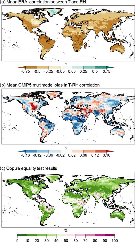
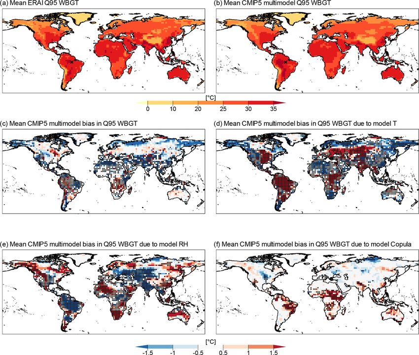
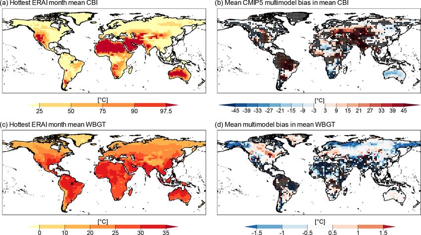
R. Villalobos-Herrera et al.: Towards a compound-event-oriented climate model evaluation                                             1873

Figure 2. Mean fire hazard index (CBI) value for ERA-Interim (a), and mean multimodel bias in mean CBI (b). Note that the palette is
non-linear, as it follows typical defined ranges of fire hazard levels based on the CBI, i.e. very low, low, moderate, high, very high, and
extreme. Mean heat stress index (WBGT) value for ERA-Interim (c), and mean multimodel bias in mean WBGT (d). Stippling indicates
locations where at least 75 % of CMIP5 models failed the AD two-sample test between the CMIP5 and ERA-Interim distributions of CBI
and WBGT. Bias was calculated as (CMIP5 minus ERA-Interim).

Figure 3. Mean temperature (T ) of the hottest month in ERA-Interim reanalysis (a), mean CMIP5 multimodel bias in mean temperature (b),
mean relative humidity (RH) of ERA-Interim reanalysis (c), and mean CMIP5 multimodel bias in mean RH (d). Stippling indicates locations
where at least 75 % of models failed the AD two-sample test between the CMIP5 and ERA-Interim marginal distributions of T and RH. Bias
was calculated as (CMIP5 minus ERA-Interim).

https://doi.org/10.5194/nhess-21-1867-2021                                     Nat. Hazards Earth Syst. Sci., 21, 1867–1885, 2021
1874                          R. Villalobos-Herrera et al.: Towards a compound-event-oriented climate model evaluation

tistical dependence. We first confirm that the expected lat-
itudinal variation in T is present in ERA-Interim reanaly-
sis (Fig. 3a) and that RH is low over known desertic areas
(Fig. 3c).
   The spatial pattern of mean T is well represented by
CMIP5 models (Fig. A3c), with all models showing a pat-
tern correlation over land with ERA-Interim above 0.93, con-
sistent with an acceptable representation of the first-order
global-scale atmospheric circulation. However, significant
differences in the representation of the distributions (based
on the AD test) are found over the Amazon basin, where
the multimodel mean bias in mean T is positive, and over
Northern Africa and the Middle East, where the bias in mean
T is negative (Fig. 3b). Overall, we found that the area-
weighted multimodel mean of the absolute value of the T
bias is 1.6 ◦ C. The AD test results show that CMIP5 models
fail to reproduce the observed ERA-Interim distribution of T
over 40 % of the global land mass.
   We find worse model skills in representing the RH dis-
tribution; in fact, models failed the AD test over 59 % of the
global land mass (Fig. 3d). The spatial pattern of RH is not as
well represented as that of T , with minimum and maximum
pattern correlations of 0.75 and 0.90, respectively (Fig. A3d).
The mean multimodel bias in RH is particularly large in the
Amazon basin. Nevertheless, there are areas where the bias
is relatively small, e.g. in Australia, the Sahara, and eastern
Asia. Notably, there is a clear resemblance between the bias
patterns of mean RH (Fig. 3d) and CBI (Fig. 2b), with re-
gions with high positive bias in RH corresponding to regions
with strong negative bias in CBI, and an identical percent-
age of land mass showing significant differences. No similar
behaviour is found for WBGT; i.e. the WBGT bias spatial
pattern is similar neither to that of T nor RH bias. We will
investigate this behaviour in CBI and WBGT in further detail
in Sect. 4.3.

4.2    Dependence between T and RH                                Figure 4. Mean ERA-Interim correlation (τ ) between T and
                                                                  RH (a), mean CMIP5 multimodel bias in τ (b), and the proportion
The results for our tests on the dependency structure of T        of CMIP5 samples where the copula equality was rejected (c). Stip-
and RH in CMIP5 models are shown in Fig. 4. Figure 4a             pling in panel (b) indicates locations where the correlations of more
and b show Kendall’s τ correlation between T and RH based         than 75 % of CMIP5 model samples have significantly different
on ERA-Interim reanalysis and the mean multimodel bias of         values compared to ERA-Interim, as calculated using Bonferroni-
this correlation, respectively. T and RH are strongly nega-       corrected p values. Bias was calculated as (CMIP5 minus ERA-
tively correlated (Fig. 4a), with an area-weighted mean value     Interim).
of −0.50 (virtually all land mass has a significant correla-
tion; not shown are results based on the indepTest function
                                                                  (Fig. 4c), with an over 80 % agreement in copula structure
of the copula R package; v0.999–19.1; Hofert et al., 2018).
                                                                  between ERA-Interim and models for 52 % of land masses
The presence of a negative correlation is illustrated in Fig. 1
                                                                  and 60 %–80 % agreement in 33 % of land masses. Overall,
(and A1 for a representative location). The area-weighted ab-
                                                                  the regions where we detect the highest amount of statisti-
solute mean multimodel bias in τ is 0.095. The bias in τ is
                                                                  cally significant differences in the copula structure and τ in-
not significant for most of the global land mass for most of
                                                                  clude parts of the Horn of Africa, India, and the Amazon
the models; i.e. the modelled correlations lie within the 95 %
                                                                  basin (see also Fig. A1c and d, where the model values have
confidence interval of τ of ERA-Interim (see infrequent stip-
                                                                  different distributions compared to ERA-Interim).
pling over 5.3 % and 9.3 % of land masses in Figs. 4b and A4,
respectively). Results are similar for the copula equality test

Nat. Hazards Earth Syst. Sci., 21, 1867–1885, 2021                                 https://doi.org/10.5194/nhess-21-1867-2021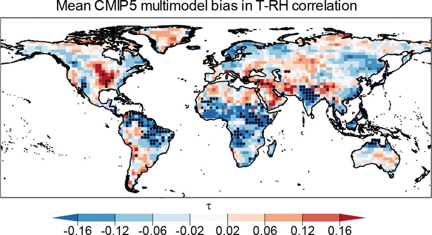
R. Villalobos-Herrera et al.: Towards a compound-event-oriented climate model evaluation 1875
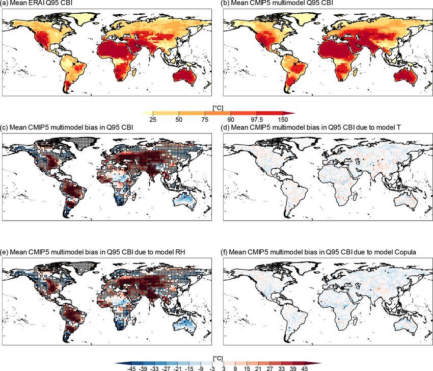
Figure 5. ERA-Interim (a) and CMIP5 multimodel mean (b) 95th quantile CBI values. Note that the palette is non-linear, as it follows typical
defined ranges of fire hazard levels based on the CBI, i.e. very low, low, moderate, high, very high, and extreme. Mean CMIP5 multimodel
bias in Q95 CBI (c), and its decomposition into bias due to the T (d), RH (e), and copula (f) components of the models. Stippling indicates
locations where more than 75 % of CMIP5 model sample values lie outside the 95 % confidence interval for ERA-Interim estimated based
on bootstrap samples. Bias was calculated as (CMIP5 or transformation minus ERA-Interim).
4.3 Contribution of the bias in the drivers to the bias in fact, the stippling over 75 % of land masses in Fig. 5c indi-
CBI and WBGT extremes cates that the models differ significantly from ERA-Interim.
The bias in RH is the main contributor to total mean bias
in extreme CBI values (Fig. 6d–f). The relevance of RH for
4.3.1 Drivers of the biases in CBI extremes
the bias in CBI is visible from the similarities in magnitude
and spatial distribution of bias between Fig. 5c and e. Fur-
We now assess the biases in the representation of extreme thermore, while the area-weighted mean of absolute bias in
events (95th quantile, Q95) in the CBI index and the associ- CBI is 21 ◦ C, the corresponding mean biases due to T , RH,
ated drivers of the biases (Fig. 5). The spatial pattern of the and the dependency between them are 3, 20, and 3 ◦ C, re-
CMIP5 multimodel mean of Q95 (Fig. 5b) is very similar to spectively. The relevant contribution of RH to the CBI index
that of ERA-Interim (Fig. 5a). Figure 5c shows the biases bias is consistent with the definition of the index, which is
in extreme CBI, whose highest values are in South Amer- mainly influenced by RH and to a lesser extent by T (see
ica, central North America, and parts of central Asia, which nearly horizontal CBI isolines in Fig. 1); hence, also the de-
is in line with the biases in mean CBI (Fig. 2b). The area- pendency between T and RH plays a negligible role. As a
weighted mean of absolute bias in the CMIP5 model CBI result, while RH bias contributions drive significant biases in
is 21 ◦ C, which is large compared to the area-weighted mean CBI about everywhere but in the Sahara and Australia (see
CBI in ERA-Interim of 84 ◦ C (i.e. corresponding to 25 %). In stippling over 73 % of land masses in Fig. 5c), T and de-
https://doi.org/10.5194/nhess-21-1867-2021 Nat. Hazards Earth Syst. Sci., 21, 1867–1885, 2021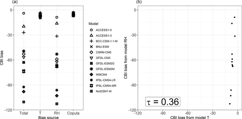
1876                          R. Villalobos-Herrera et al.: Towards a compound-event-oriented climate model evaluation

pendence do not drive significant biases in CBI (see near-         ever, the total bias in WBGT is only significant over 39 % of
complete absence of stippling in Fig. 5d and f).                   land masses. Further evidence for these compensating biases
   A closer examination of the bias decomposition results          can be found by observing that the area-weighted average
shows, for a site with large positive bias in Brazil, that the     of absolute bias in Q95 WBGT, i.e. 1.1 ◦ C, is smaller than
results shown in the multimodal mean bias plots (Fig. 5c           the contributions from T and RH, i.e. 1.9 and 1.4 ◦ C, respec-
and e) reflect intermodel model behaviour at the local level.      tively. In addition, we observe a tendency towards a lower
That is, CMIP5 models with high RH bias contributions also         bias, on average, driven by the copula component (global
show high overall CBI bias (Fig. 6a). At this location, there      area-weighted average of absolute bias equal to 0.85 ◦ C);
is a positive intermodel correlation between the biases driven     note that, however, some relevant positive bias contributions
by T and RH (τ = 0.82; Fig. 6b). Such behaviour is due to          exist over eastern Brazil and central Africa, where the cop-
the combination of the following two reasons: (1) a nega-          ula test shows higher frequencies of rejection (Fig. 4c), and
tive intermodel correlation between the biases in T and RH,        a negative contributions over northern Russia, the central
i.e. CMIP5 models simulating temperatures that are too high        United States, and eastern Europe (Fig. 7f).
also tend to simulate relative humidity that is too low (as dis-      The compensating bias in T and RH found above is in
cussed by Fischer and Knutti, 2013); and (2) the fact that         line with the findings of Fischer and Knutti (2013). Their
CBI is high for low RH and high T . This feature is discussed      results indicate that, at the local scale and for individual
in more detail in Sect. 5. Similar results to those discussed      models, the biases in WBGT driven by T and RH tend to
above for the site in Brazil are also observed for another rep-    cancel each other out, resulting in small biases in the heat
resentative location in South Africa with large negative bias      stress index. We find that this behaviour in individual mod-
in CBI (Fig. A5a). These locations are indicated throughout        els is reflected in the multimodel mean result (Fig. 7c) in re-
map plots with X markers.                                          gions where most models have similar behaviours, e.g. where
                                                                   most models show a positive WBGT bias contribution from
4.3.2   Drivers of the biases in WBGT extremes                     T (Fig. 7d) and a negative one from RH (Fig. 7e). We con-
                                                                   firm the behaviour in individual models for two representa-
The spatial pattern of Q95 in ERA-Interim (Fig. 7a) and in         tive locations. In Brazil, the small mean bias in WBGT Q95
the CMIP5 multimodel mean (Fig. 7b) is similar, with low           for all CMIP5 models results from mostly positive and neg-
values concentrated along mountain ranges such as the An-          ative biases driven by T and RH, respectively, across models
des and Himalayas and in high latitudes and with the high-         (Fig. 8a; the figure also indicates that the bias driven by the
est values located in South America and the Indian subcon-         dependence is small and positive). In particular, models af-
tinent. In several regions worldwide, CMIP5 models tend to         fected by a positive T bias contribution in WBGT because of
underestimate Q95 values of WBGT (global area-weighted             T that is too high tend also to be affected by a negative RH
mean bias of −0.35 ◦ C) and show significant biases relative       bias contribution because of RH that is too low (Fig. 8b). The
to ERA-Interim along the tropics and subtropics (Fig. 7c).         compensation of the biases in individual models arises from
However, in terms of values of the bias, the CMIP5 repre-          (1) opposite biases in T and RH (models simulating tempera-
sentation of the WBGT appears better than that of CBI. The         tures that are too high also tend to simulate relative humidity
area-weighted mean of absolute bias in the index is 1.1 ◦ C        that is too low; Fischer and Knutti, 2013) and (2) the WBGT
(Fig. 7c), which is small compared to the area-weighted            tendency to be high (low) for humid and warm (dry and cold)
mean WBGT in ERA-Interim, i.e. 29 ◦ C (Fig. 7a).                   conditions. Figure A6 illustrates such a cancellation of the
   The decomposition of the bias shows that unlike CBI there       bias in WBGT for a location in South Africa, where the neg-
is no single dominating source of bias in extreme values of        ative dependency between T and RH leads to a small bias
WBGT (Fig. 7d–f); all three possible sources contribute to         in WBGT. In this location, the model biases driven by T are
the overall bias. Importantly, a degree of compensating bi-        negative; therefore those driven by RH are positive.
ases is evident when comparing the multimodel mean biases
driven by T (Fig. 7d) and RH (Fig. 7e). Large biases of oppo-
site signs are evident over South America, central Asia, and       5   Discussion
other land masses; hence, in these areas, the resulting biases
                                                                   Our results underline the importance of understanding the
in WBGT tend to be small (Fig. 7c). Significant but opposite
                                                                   sources of the biases in hazard indicators through multivari-
biases in T and RH (see stippling in Fig. 7d and e) result in
                                                                   ate procedures. In fact, hazard indicators can have biases re-
nonsignificant biases in WBGT (Fig. 7c) over regions such
                                                                   sulting from a complex combination of biases in the driving
as North America’s Mississippi basin and around Zaire in
                                                                   variables of the indicator and in biases in the dependence be-
central Africa. Globally, this compensating behaviour can be
                                                                   tween the variables. We find that biases in CBI extremes are
observed in the percentages of land masses where each bias
                                                                   mainly driven by biases in relative humidity, while biases in
component is significant. T - and RH-driven biases are sig-
                                                                   WBGT extremes are often driven by biases in temperature,
nificant over 69 % and 48 % of the global land mass, respec-
                                                                   relative humidity, and their statistical dependence.
tively, while copula biases are significant over 12 %; how-

Nat. Hazards Earth Syst. Sci., 21, 1867–1885, 2021                                https://doi.org/10.5194/nhess-21-1867-2021
R. Villalobos-Herrera et al.: Towards a compound-event-oriented climate model evaluation 1877 Figure 6. Spread of mean total bias in the 95th quantile (Q95) of CBI and its contribution from T , RH, and their copula for individual CMIP5 models (a), and a scatter plot of the T and RH contributions to Q95 CBI bias, with their Kendall rank correlation coefficient (p value < 0.001) (b). Shown are the results for a grid point in Brazil (Amazonia, 5◦ S and 56.5◦ W). Bias was calculated as (CMIP5 or transformation minus ERA-Interim). Equal axes are used in panel (b) to highlight the differences in spread between both bias components. Biases in WBGT are smaller than the bias contributions speed and previous rainfall, which are for instance included from T and RH, i.e. the biases in the two variables compen- in the Forest Fire Weather Index (FWI, Van Wagner, 1987), sate. In particular, in line with Fischer and Knutti (2013), as well as fuel availability and aridity. models which tend to simulate T that is too high also tend to The presented bias decomposition method would poten- simulate RH that is too low (and vice versa), which results in tially become even more relevant when considering more relatively smaller absolute biases in the WBGT of individual complex hazard indicators driven by more than two variables, models. A negative intermodel correlation between the con- such as the case of fire hazard as outlined above. This would tributions of T and RH to WBGT biases reduces the biases require an extension of the bivariate copula framework. For in WBGT in the CMIP5 average. For the fire hazard, despite example, in the case of three variables – X1 , X2 , and X3 – that fact that a positive intermodel correlation between the we would have to investigate the behaviour of marginals, the bias driven by T and RH exists, no enhancement of the CBI dependence between X1 and X2 (with the two-dimensional bias occurs because the index is mainly controlled by RH copula C12 ), X2 and X3 (C23 ), and X1 and X3 (C13 ), and (see isolines in Fig. 1c), which also controls the bias of the then the joint behaviour of the three variables with the three- index. The WBGT index shows additional complexity due to dimensional copula (C123 ). Alternatively, vine copula de- the contribution of the biases in the copula between T and compositions could be employed (Hobæk Haff et al., 2015). RH in areas such as eastern Brazil, Africa, and parts of cen- Similar considerations apply for the consideration of tem- tral North America and India. poral dependencies. The analysis can be done using both a These findings exemplify the need for multivariate bias ad- parametric or non-parametric approach. For instance, in Vez- justment methods, which can adjust climate model biases in zoli et al. (2017), a non-parametric approach has been used the dependencies between multiple drivers of hazards (Fran- to analyse the behaviour of the three variables precipitation, cois et al., 2020; Vrac, 2018). Furthermore, relying on cli- temperature, and runoff. mate models that plausibly represent large-scale atmospheric Given the critical importance of addressing com- circulation (Maraun, 2016; Maraun et al., 2017) would im- pound/multivariate events that are often associated with ex- prove our confidence in the simulation of multivariate haz- treme impacts (Leonard et al., 2014; Zscheischler et al., ards. The relevance of multivariate bias adjustment methods 2018), we assessed the bias decomposition for high quan- is also supported by the fact that adjusting biases variable tiles of CBI and WBGT. The extremes of the considered in- by variable may even increase biases in impact-relevant indi- dicators are not necessarily caused by extreme values of the cators (Zscheischler et al., 2019). Nevertheless, in line with drivers. Hence, the characterization of the dependence struc- our findings, Zscheischler et al. (2019) found that univari- ture between their climate drivers (i.e. T and RH) was per- ate bias adjustment is relatively efficient in the case of CBI, formed in terms of their full joint distribution to capture all while multivariate methods lead to much stronger reductions the events; i.e. we did not only consider the combination of in the case of WBGT. It should be noted, however, that the simultaneous T and RH extremes. However, depending on considered fire indicator CBI is overly simplistic. In practice, the type of hazard considered, investigating biases in the tail weather conditions that promote fires are also related to wind dependence between the drivers may be relevant to under- https://doi.org/10.5194/nhess-21-1867-2021 Nat. Hazards Earth Syst. Sci., 21, 1867–1885, 2021
1878                            R. Villalobos-Herrera et al.: Towards a compound-event-oriented climate model evaluation

Figure 7. ERA-Interim (a) and CMIP multimodel mean (b) 95th quantile WBGT values. Mean CMIP5 multimodel bias in Q95 WBGT (c)
and its decomposition into bias due to the T (d), RH (e), and copula (f) components of the models. Stippling indicates locations where more
than 75 % of CMIP5 model sample values lie outside the 95 % confidence interval for ERA-Interim estimated based on bootstrap samples.
Bias was calculated as (CMIP5 or transformation minus ERA-Interim).

standing the biases in the hazard. For example, the tail de-            that proposed here, i.e. disentangling the biases in the indi-
pendence between storm surge and precipitation, which is                vidual physical drivers, could be adopted in future studies to
relevant for compound coastal flooding, may be slightly un-             aid present and future impact assessments.
derestimated in CMIP5 models (Bevacqua et al., 2019). Sim-
ilarly, there is evidence that the tail dependence between hot
and dry conditions may be underestimated by climate models              6   Conclusions
in some cases (Zscheischler and Fischer, 2020).
   The present methodology can be used for assessing the                Climate model data contain biases that need to be evaluated
sources of bias in other types of compound events (Zscheis-             and ultimately adjusted to avoid misleading risk assessments.
chler et al., 2020) caused by other sets of dependent drivers,          However, while many climate-related extreme impacts are
such as compound drought and heat (Zscheischler and                     caused by the combination of multiple variables, i.e. com-
Seneviratne, 2017) and compound coastal flooding (Bevac-                pound events, climate model evaluation methods typically
qua et al., 2020b). Other types of compound events, e.g. tem-           do not consider the multivariate nature of the hazards. In
poral clustering of storms (Bevacqua et al. 2020c; Priestley            this study, we took a compound event perspective and, based
et al., 2017) and simultaneous extreme events in distant re-            on copula theory, introduced a multivariate bias-assessment
gions (Kornhuber et al., 2020) can also lead to large im-               framework, which allows for disentangling and better under-
pacts and are therefore relevant for the impact community.              standing the multiple sources of biases in hazard indicators.
A compound-event-oriented evaluation of impacts similar to              Through a non-parametric procedure, here we investigated

Nat. Hazards Earth Syst. Sci., 21, 1867–1885, 2021                                      https://doi.org/10.5194/nhess-21-1867-2021
R. Villalobos-Herrera et al.: Towards a compound-event-oriented climate model evaluation                                            1879

Figure 8. Spread of mean total bias in the 95th quantile (Q95) of WBGT and its contribution from T , RH, and their copula for individual
CMIP5 models (a), and a scatter plot of the T and RH contributions to Q95 WBGT bias, with their respective Kendall rank correlation
coefficient (p value < 0.001). Shown are results for a grid point in Brazil (Amazonia, 5◦ S and 56.5◦ W). Bias was calculated as (CMIP5 or
transformation minus ERA-Interim). Equal axes are used in panel (b) to highlight the differences in spread between both bias components.

how the biases in temperature, relative humidity, and their               Given the relevance of compound weather and climate
dependence affect the overall biases in fire and heat stress           events for societal impacts, the presented framework could
indicators (CBI and WBGT, respectively). We found that bi-             be useful in further studies aiming at disentangling and bet-
ases in CBI are mainly driven by biases in relative humidity,          ter understanding the drivers of the biases in the represen-
in line with the fact that the index is only marginally affected       tations of other impacts. The framework could also be use-
by temperature. In contrast, the biases in WBGT are often              ful to assess biases among drivers of hazards when data for
driven by biases in temperature, relative humidity, and their          the hazard indicators are not available. A compound-event-
statistical dependence (e.g. in areas including eastern Brazil,        oriented model evaluation of modelled impacts and associ-
Africa, and parts of central North America and India). Op-             ated drivers would be beneficial for disaster risk reduction
posing biases in temperature and relative humidity tend to             and, ultimately, could feed back into climate model develop-
compensate for each other, resulting in relatively small bi-           ment processes and stimulate the design of new bias adjust-
ases in WBGT. The results highlight areas where a careful              ment methods.
interpretation of these indicators is required and where multi-
variate bias corrections of temperature and relative humidity
should be considered future risk assessments.

https://doi.org/10.5194/nhess-21-1867-2021                                     Nat. Hazards Earth Syst. Sci., 21, 1867–1885, 2021
1880                            R. Villalobos-Herrera et al.: Towards a compound-event-oriented climate model evaluation

Appendix A: Information

Figure A1. Samples of hourly 2 m air T (◦ C) vs. RH (%) during the period 1979–2005 for ERA-Interim reanalysis (grey points) and four
models (black points) from the CMIP5 multimodel ensemble (BNU-ESM (a), GFDL-CM3 CNRM-CM5 (b), GFDL-CM3 (c), and IPSL-
CM5A-LR (d)) for a grid point in Brazil (Amazonia, 5◦ S and 56.5◦ W) indicated throughout map plots in the Results section (Sect. 4) with
X markers. The isolines illustrate equal levels of the hazard indices of fire (orange) and heat stress (green), corresponding to CBI and WBGT
indices, respectively, which are both functions of T and RH.

Nat. Hazards Earth Syst. Sci., 21, 1867–1885, 2021                                        https://doi.org/10.5194/nhess-21-1867-2021
R. Villalobos-Herrera et al.: Towards a compound-event-oriented climate model evaluation                                              1881

Figure A2. Block diagram showing the data and methods used. Temperature (T ) and relative humidity (RH) decorrelated samples from
CMIP5 models’ biases are analysed using univariate and multivariate statistical tests using ERA-Interim as reference dataset. We also create
transformed CMIP5 model samples, which allow for assessing the bias in the extreme values of the hazard indicator (CBI and WBGT) driven
by biases in T , RH, and their statistical dependence.

Figure A3. CMIP5 multimodel mean fire hazard index (CBI) value (a), heat stress index (WBGT) value (b), temperature (T ) value (c), and
relative humidity (RH) (d).

https://doi.org/10.5194/nhess-21-1867-2021                                      Nat. Hazards Earth Syst. Sci., 21, 1867–1885, 2021
1882                            R. Villalobos-Herrera et al.: Towards a compound-event-oriented climate model evaluation

Figure A4. As Fig. 4b but where stippling indicates locations where more than 75 % of CMIP5 model sample values lie outside the 95 %
confidence interval for ERA-Interim.

Figure A5. As Fig. 6 for a grid point in South Africa (32.5◦ S and 23.5◦ E), with Kendall rank correlation p value = 0.12.

Figure A6. As Fig. 8 for a grid point in South Africa (32.5◦ S and 23.5◦ E), with Kendall rank correlation p value = 0.063.

Nat. Hazards Earth Syst. Sci., 21, 1867–1885, 2021                                       https://doi.org/10.5194/nhess-21-1867-2021
R. Villalobos-Herrera et al.: Towards a compound-event-oriented climate model evaluation                                                1883

Data availability. Data from CMIP5 models are available from            References
the Earth System Grid Federation (ESGF) peer-to-peer system
(https://esgf-node.llnl.gov/projects/cmip5, last access: June 2021)
(WCRP, 2021). The ERA-Interim reanalysis dataset is available           ASCM – American College of Sports Medicine: Prevention of Ther-
from the ECMWF Public Datasets web page (https://apps.ecmwf.              mal Injuries During Distance Running – Position stand, Med.
int/datasets/, last access: June 2021) (ECMWF, 2021).                     Sci. Sport. Exerc., 16, ix–xiv, 1984.
                                                                        Berrisford, P., Kållberg, P., Kobayashi, S., Dee, D., Uppala, S., Sim-
                                                                          mons, A. J., Poli, P., and Sato, H.: Atmospheric conservation
Author contributions. EB and CDM conceived the study and su-              properties in ERA-Interim, Q. J. Roy. Meteor. Soc., 137, 1381–
pervised the project. RVH carried out the analysis of the biases          1399, https://doi.org/10.1002/qj.864, 2011.
based on the data prepared by EB, AFSR, LC, GA, BM, and MH.             Bevacqua, E., Maraun, D., Hobæk Haff, I., Widmann, M.,
RVH prepared all the figures except Figs. 1 and A1, which were pre-       and Vrac, M.: Multivariate statistical modelling of compound
pared by EB and AR. The paper was written by GA, EB, CDM, AR,             events via pair-copula constructions: analysis of floods in
and RVH. JZ contributed to the development of the idea of the work        Ravenna (Italy), Hydrol. Earth Syst. Sci., 21, 2701–2723,
and helped with final edits. All the authors discussed the results of     https://doi.org/10.5194/hess-21-2701-2017, 2017.
the paper.                                                              Bevacqua, E., Maraun, D., Vousdoukas, M. I., Voukouvalas, E.,
                                                                          Vrac, M., Mentaschi, L., and Widmann, M.: Higher probability
                                                                          of compound flooding from precipitation and storm surge in Eu-
                                                                          rope under anthropogenic climate change, Science Advances, 5,
Competing interests. The authors declare that they have no conflict
                                                                          9, eaaw5531, https://doi.org/10.1126/sciadv.aaw5531, 2019.
of interest.
                                                                        Bevacqua, E., Vousdoukas, M. I., Shepherd, T. G., and Vrac,
                                                                          M.: Brief communication: The role of using precipitation
                                                                          or river discharge data when assessing global coastal com-
Special issue statement. This article is part of the special issue        pound flooding, Nat. Hazards Earth Syst. Sci., 20, 1765–1782,
“Understanding compound weather and climate events and related            https://doi.org/10.5194/nhess-20-1765-2020, 2020a.
impacts (BG/ESD/HESS/NHESS inter-journal SI)”. It is not asso-          Bevacqua, E., Vousdoukas, M. I., Zappa, G., Hodges, K., Shepherd,
ciated with a conference.                                                 T. G., Maraun, D., Mentaschi, L., and Feyen, L.: More meteo-
                                                                          rological events that drive compound coastal flooding are pro-
                                                                          jected under climate change, Commun. Earth Environ., 1, 47,
Acknowledgements. This work emerged from the Training School              https://doi.org/10.1038/s43247-020-00044-z, 2020b.
on Statistical Modelling Compound Events organized by the Eu-           Bevacqua, E., Zappa, G., and Shepherd, T. G.: Shorter cy-
ropean COST Action DAMOCLES (CA17109). We acknowledge                     clone clusters modulate changes in European wintertime
the World Climate Research Programme Working Group on Cou-                precipitation extremes, Environ. Res. Lett., 15, 124005,
pled Modelling, which is responsible for CMIP, and we thank the           https://doi.org/10.1088/1748-9326/abbde7, 2020c.
climate modelling groups for producing and making available their       Brando, P. M., Balch, J. K., Nepstad, D. C., Morton, D. C., Putz,
model output.                                                             F. E., Coe, M. T., Silvério, D., Macedo, M. N., Davidson,
                                                                          E. A., Nóbrega, C. C., Alencar, A., and Soares-Filho, B. S.:
                                                                          Abrupt increases in Amazonian tree mortality due to drought-
Financial support. Emanuele Bevacqua was supported by the                 fire interactions, P. Natl. Acad. Sci. USA, 111, 6347–6352,
European Research Council grant ACRCC (project 339390)                    https://doi.org/10.1073/pnas.1305499111, 2014.
and the DOCILE project (NERC grant NE/P002099/1). An-                   Dale, M. and Fortin, M.: Spatial Autocorrelation and Statistical
dreia F. S. Ribeiro was supported by the Portuguese Foundation            Tests: Some Solutions, J. Agr. Biol. Envir. St., 14, 188–206,
for Science and Technology (FCT) (grant PD/BD/114481/2016),               2009.
the project IMPECAF (PTDC/CTA-CLI/28902/2017), and the                  Dee, D. P., Uppala, S. M., Simmons, A. J., Berrisford, P., Poli,
Swiss National Science Foundation (project number 186282).                P., Kobayashi, S., Andrae, U., Balmaseda, M. A., Balsamo, G.,
Carlo De Michele was supported by the Italian Ministry of Ed-             Bauer, P., Bechtold, P., Beljaars, A. C. M., van de Berg, L., Bid-
ucation, University and Research through the PRIN2017 RE-                 lot, J., Bormann, N., Delsol, C., Dragani, R., Fuentes, M., Geer,
LAID project. The work of Laura Crocetti was supported by the             A. J., Haimberger, L., Healy, S. B., Hersbach, H., Hólm, E. V.,
TU Wien Wissenschaftspreis 2015, awarded to Wouter Dorigo.                Isaksen, L., Kållberg, P., Köhler, M., Matricardi, M., McNally,
Roberto Villalobos-Herrera was supported by the University of             A. P., Monge-Sanz, B. M., Morcrette, J.-J., Park, B.-K., Peubey,
Costa Rica and the Newcastle University School of Engineering.            C., de Rosnay, P., Tavolato, C., Thépaut, J.-N., and Vitart, F.: The
Jakob Zscheischler was supported by the Swiss National Science            ERA-Interim reanalysis: configuration and performance of the
Foundation (Ambizione grant 179876) and the Helmholtz Initiative          data assimilation system, Q. J. Roy. Meteor. Soc., 137, 553–597,
and Networking Fund (Young Investigator Group COMPOUNDX,                  https://doi.org/10.1002/qj.828, 2011.
grant agreement VH-NG-1537).                                            Durante, F. and Sempi, C.: Principles of Copula Theory, 1st Edn.,
                                                                          Chapman and Hall/CRC, https://doi.org/10.1201/b18674, 2015.
                                                                        ECMWF: Public Datasets, available at: https://apps.ecmwf.int/
Review statement. This paper was edited by Ricardo Trigo and re-          datasets/, last access: June 2021.
viewed by Mathieu Vrac and one anonymous referee.                       FIALA, D., Havenith, G., Bröde, P., Kampmann, B., and Jendritzky,
                                                                          G.: UTCI-Fiala multi-node model of human heat transfer and

https://doi.org/10.5194/nhess-21-1867-2021                                     Nat. Hazards Earth Syst. Sci., 21, 1867–1885, 2021
You can also read