Recovering 3D Human Pose from Monocular Images
←
→
Page content transcription
If your browser does not render page correctly, please read the page content below
IEEE TRANSACTIONS ON PATTERN ANALYSIS AND MACHINE INTELLIGENCE. SUBMITTED FOR REVIEW.                                                  1

                        Recovering 3D Human Pose from
                               Monocular Images
                                                  Ankur Agarwal and Bill Triggs

   Abstract— We describe a learning based method for recovering        model [9, 23]. In contrast, learning based approaches try to
3D human body pose from single images and monocular image              avoid the need for explicit initialization and accurate 3D
sequences. Our approach requires neither an explicit body model        modelling and rendering, and to capitalize on the fact that
nor prior labelling of body parts in the image. Instead, it recovers
pose by direct nonlinear regression against shape descriptor           the set of typical human poses is far smaller than the set of
vectors extracted automatically from image silhouettes. For            kinematically possible ones, by estimating (learning) a model
robustness against local silhouette segmentation errors, silhouette    that directly recovers pose estimates from observable image
shape is encoded by histogram-of-shape-contexts descriptors. We        quantities. In particular, example based methods explicitly
evaluate several different regression methods: ridge regression,       store a set of training examples whose 3D poses are known,
Relevance Vector Machine (RVM) regression and Support Vector
Machine (SVM) regression over both linear and kernel bases. The        and estimate pose by searching for training image(s) similar
RVMs provide much sparser regressors without compromising              to the given input image, and interpolating from their poses
performance, and kernel bases give a small but worthwhile              [5, 18, 22, 27].
improvement in performance. Loss of depth and limb labelling              In this paper we take a learning based approach, but
information often makes the recovery of 3D pose from single
silhouettes ambiguous. We propose two solutions to this: the first
                                                                       instead of explicitly storing and searching for similar training
embeds the method in a tracking framework, using dynamics              examples, we use sparse Bayesian nonlinear regression to
from the previous state estimate to disambiguate the pose;             distill a large training database into a single compact model
the second uses a mixture of regressors framework to return            that has good generalization to unseen examples. Given the
multiple solutions for each silhouette. We show that the resulting     high dimensionality and intrinsic ambiguity of the monocular
system tracks long sequences stably, and is also capable of
accurately reconstructing 3D human pose from single images,
                                                                       pose estimation problem, the selection of appropriate image
giving multiple possible solutions in ambiguous cases. For realism     features and good control of overfitting is critical for success.
and good generalization over a wide range of viewpoints, we train      We are not aware of previous work on pose estimation that
the regressors on images resynthesized from real human motion          directly addresses these issues. Our strategy is based on the
capture data. The method is demonstrated on a 54-parameter             sparsification and generalization properties of our nonlinear
full body pose model, both quantitatively on independent but
similar test data, and qualitatively on real image sequences. Mean
                                                                       regression algorithm, which is a form of the Relevance Vector
angular errors of 4–5 degrees are obtained — a factor of 3 better      Machine (RVM) [29]. RVMs have been used earlier, e.g.
than the current state of the art for the much simpler upper body      to build kernel regressors for 2D displacement updates in
problem.                                                               correlation-based patch tracking [33]. Human pose recovery is
  Index Terms— Computer vision, human motion estimation,               significantly harder — more ill-conditioned and nonlinear and
machine learning, multivariate regression, Relevance Vector Ma-        much higher dimensional — but by selecting a sufficiently rich
chine                                                                  set of image descriptors, it turns out that we can still obtain
                                                                       enough information for successful regression. Loss of depth
                                                                       and limb labelling information often makes the recovery of
                       I. I NTRODUCTION
                                                                       3D pose from single silhouettes ambiguous. We propose two
   We consider the problem of estimating and tracking 3D               solutions to this. The first embeds the method in a tracking
configurations of complex articulated objects from monocular           framework, using dynamics from the previous state estimate
images, e.g. for applications requiring 3D human body pose             to disambiguate the pose. The second uses a mixture of
and hand gesture analysis. There are two main schools of               regressors framework to return multiple possible solutions for
thought on this. Model-based approaches presuppose an ex-              each silhouette, allowing accurate pose reconstructions from
plicitly known parametric body model, and estimate the pose            single images. When working with a sequence of images, these
either by directly inverting the kinematics (which has many            solutions are fed as input to a multiple hypothesis tracker to
possible solutions and requires known image positions for each         give the most likely estimate for each time step.
body part) [28], or by numerically optimizing some form of
model-image correspondence metric over the pose variables,             Previous work: There is a good deal of prior work on
using a forward rendering model to predict the images (which           human pose analysis, but relatively little on directly learning
is expensive and requires a good initialization, and the problem       3D pose from image measurements. Brand [8] models a
always has many local minima [25]). An important sub-                  dynamical manifold of human body configurations with a
case is model-based tracking, which focuses on tracking the            Hidden Markov Model and learns using entropy minimization,
pose estimate from one time step to the next starting from             Athitsos and Sclaroff [4] learn a perceptron mapping between
a known initialization, based on an approximate dynamical              the appearance and parameter spaces, and Shakhnarovich et al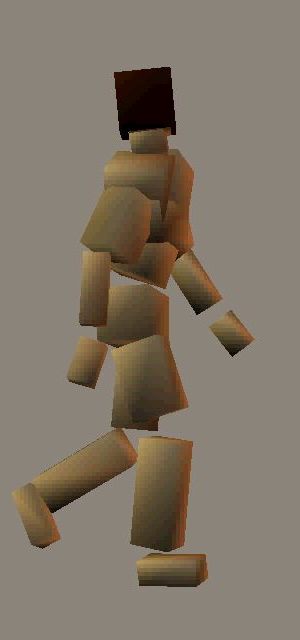
IEEE TRANSACTIONS ON PATTERN ANALYSIS AND MACHINE INTELLIGENCE. SUBMITTED FOR REVIEW.                                               2

                                                                    P
[22] use an interpolated-k-nearest-neighbor learning method.           k ak φk (z) of a prespecifed set of scalar basis functions
Human pose is hard to ground truth, so most papers in this          {φk (z) | k = 1 . . . p}. In our tracking framework, to help to
area [4, 8, 18] use only heuristic visual inspection to judge       disambiguate pose in cases where there are several possible
their results. However Shakhnarovich et al [22] used a human        reconstructions, the functional form is extended to include an
model rendering package (P OSER from Curious Labs) to               approximate preliminary pose estimate x̌, x = r(x̌, z). (See
synthesize ground-truthed training and test images of 13 d.o.f.     section V.) At each time step, a state estimate x̌t is obtained
upper body poses with a limited (±40◦ ) set of random torso         from the previous two pose vectors using an autoregressive dy-
movements and view points. In comparison, our regression            namical model, and this is used to compute the basis functions,
algorithm estimates full body pose and orientation (54 d.o.f.)      which now take the form {φk (x̌, z) | k = 1 . . . p}. Section
— a problem whose high dimensionality would really stretch          VI gives an alternative method for handling ambiguities by
the capacity of an example based method such as [22]. Like          returning multiple possible 3D configurations corresponding to
[11, 22], we used P OSER to synthesize a large set of training      a silhouette. The Pfunctional form is extended to a probabilistic
and test images from different viewpoints, but rather than using    mixture p(x) ∼ k πk δ(x, rk ) allowing each reconstruction
random synthetic poses, we used poses taken from real human         rk to output a different solution.
motion capture sequences. Our results thus relate to real data.        Our solutions are well-regularized in the sense that the
   Several publications have used the image locations of the        weight vectors ak are damped to control over-fitting, and
centre of each body joint as an intermediate representation,        sparse in the sense that many of them are zero. Sparsity occurs
first estimating these centre locations in the image, then          because the RVM actively selects only the ‘most relevant’
recovering the 3D pose from them. Howe et al [12] develop           basis functions — the ones that really need to have nonzero
a Bayesian learning framework to recover 3D pose from               coefficients to complete the regression successfully. A sparse
known centres, based on a training set of pose-centre pairs         solution obtained by the RVM allows the system to select
obtained from resynthesized motion capture data. Mori &             relevant input features (components) in case of a linear basis
Malik [18] estimate the centres using shape context image           (φk (z) = k th component of z). For a kernel basis — φk (z) ≡
matching against a set of training images with pre-labelled         K(z, zk ) for some kernel function K(zi , zj ) and centres zk —
centres, then reconstruct 3D pose using the algorithm of            relevant training examples are selected, allowing us to prune
[28]. These approaches show that using 2D joint centres as          a large training dataset and retain only a minimal subset.
an intermediate representation can be an effective strategy,
                                                                    Organization: §II describes our image descriptors and body
but we have preferred to estimate pose directly from the
                                                                    pose representation. §III gives an outline of our regression
underlying local image descriptors as we feel that this is likely
                                                                    methods. §IV details the recovery of 3D pose from single
to prove both more accurate and more robust, also providing
                                                                    images using this regression, discussing the RVM’s feature
a generic framework for directly estimating and tracking any
                                                                    selection properties but showing that ambiguities in estimating
prespecified set of parameters from image observations.
                                                                    3D pose from single images cause occasional ‘glitches’ in
   As regards tracking, some approaches have learned dynami-        the results. §V describes our first solution to this problem:
cal models for specific human motions [19,20]. Particle filters     a tracking based regression framework capable of resolving
and MCMC methods have been widely used in probabilistic             these ambiguities, with results from our novel tracker in §V-B.
tracking frameworks e.g. [23,31]. Most of these methods use         §VI describes an alternative solution: a mixture of regressors
an explicit generative model to compute observation likeli-         based approach incorporated in a multiple hypothesis tracker.
hoods. We propose a discriminatively motivated framework            Finally, §VII concludes with some discussions and directions
in which dynamical state predictions are directly fused with        for future work.
descriptors computed from the observed image. Our algorithm
is related to Bayesian tracking, but we eliminate the need for
both an explicit body model that is projected to predict image             II. R EPRESENTING I MAGES AND B ODY P OSES
observations, and a corresponding error model that is used             Directly regressing pose on input images requires a robust,
to evaluate the likelihood of the observed image given this         compact and well-behaved representation of the observed
projection. A brief description of our regression based scheme      image information and a suitable parametrization of the body
is given is [1] and its first extension to resolve ambiguities      poses that we wish to recover. To encode the observed images
using dynamics within the regression is described in [2].           we use robust descriptors of the shape of the subject’s image
                                                                    silhouette, and to describe our body pose, we use vectors of
Overview of the approach: We represent 3D body pose by              joint angles.
55-D vectors x including 3 joint angles for each of the 18 ma-
jor body joints. This choice corresponds to the motion capture
data that we use to train the system (details in section II-B).     A. Images as Shape Descriptors
The input images are reduced to 100-D observation vectors z            Silhouettes: Of the many different image descriptors that
that robustly encode the shape of a human image silhouette.         could be used for human pose estimation, and in line with
Given a set of labelled training examples {(zi , xi ) | i =         [4, 8], we have chosen to base our system on image silhouettes.
1 . . . n}, the RVM learns a smooth reconstruction function            Silhouettes have three main advantages: (i) They can be ex-
x = r(z), valid over the region spanned by the training             tracted moderately reliably from images, at least when robust
points. The function is a weighted linear combination r(z) ≡        background- or motion-based segmentation is available and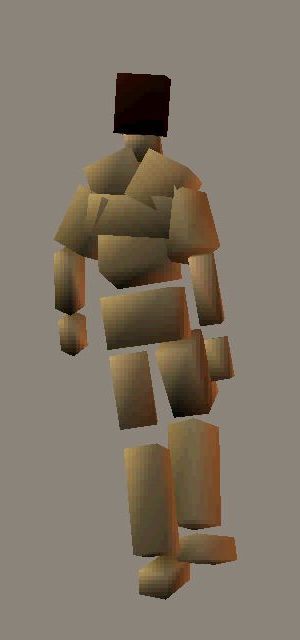
IEEE TRANSACTIONS ON PATTERN ANALYSIS AND MACHINE INTELLIGENCE. SUBMITTED FOR REVIEW. 3
0.25 0.25
0.2 0.2
0.15 0.15
0.1 0.1
0.05 0.05
0 0
−0.05 −0.05
−0.1 −0.1
−0.15 −0.15
−0.2 −0.2
−0.25 −0.25
−0.2 −0.1 0 0.1 0.2 −0.2 −0.1 0 0.1 0.2
Fig. 2. (Left) The first two principal components of the distribution of
all shape context vectors from a training data sequence, with the k-means
centres superimposed. The average-over-human-silhouettes like form arises
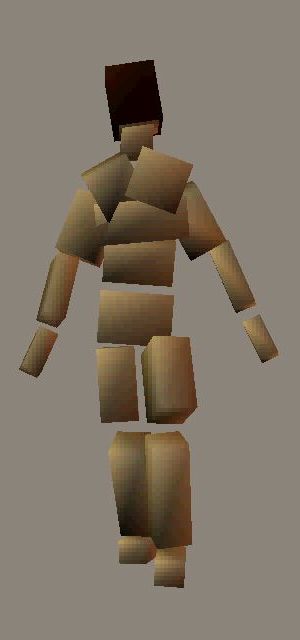
Fig. 1. Different 3D poses can have very similar image observations, causing because (besides finer distinctions) the context vectors encode approximate
the regression from image silhouettes to 3D pose to be inherently multi-valued. spatial position on the silhouette: a context at the bottom left of the silhouette
The legs are the arms are reversed in the first two images, for example. receives votes only in its upper right bins, etc. (Centre) The same projection
for the edge-points of a single silhouette (shown on the right).
problems with shadows are avoided; (ii) they are insensitive
to irrelevant surface attributes like clothing colour and texture; distribution (in fact, as a noisy multibranched curve, but we
(iii) they encode a great deal of useful information about 3D treat it as a distribution) in the 60-D shape context space. (In
pose without the need of any labelling information 1 . our implementation, shape contexts contain 12 angular × 5 ra-
Two factors limit the performance attainable from sil- dial bins, giving rise to 60 dimensional histograms.) Matching
houettes: (i) Artifacts such as shadow attachment and poor silhouettes is therefore reduced to matching these distributions
background segmentation tend to distort their local form. in shape context space. To implement this, a second level of
This often causes problems when global descriptors such as histogramming is performed: we reduce the distributions of
shape moments are used (as in [4,8]), as every local error all points on each silhouette to 100-D histograms by vector
pollutes each component of the descriptor: to be robust, shape quantizing the shape context space. Silhouette comparison is
descriptors need to have good locality. (ii) Silhouettes make thus finally reduced to a comparison of 100-D histograms.
several discrete and continuous degrees of freedom invisible The 100 centre codebook is learned once and for all by
or poorly visible (see fig. 1). It is difficult to tell frontal running k-means on the combined set of context vectors
views from back ones, whether a person seen from the side is of all of the training silhouettes. See fig. 2. (Other centre
stepping with the left leg or the right one, and what are the selection methods give similar results.) For a given silhouette,
exact poses of arms or hands that fall within (are “occluded” a 100-D histogram z is built by allowing each of its context
by) the torso’s silhouette. Including interior edge information vectors to vote softly into the few centre-classes nearest to
within the silhouette [22] is likely to provide a useful degree of it, and accumulating scores of all context vectors. This soft
disambiguation in such cases, but is difficult to disambiguate voting reduces the effects of spatial quantization, allowing
from, e.g. markings on clothing. us to compare histograms using simple Euclidean distance,
rather than, say, Earth Movers Distance [21]. (We have also
Shape Context Distributions: To improve resistance to seg- √ √
tested the normalized cellwise distance k p1 − p2 k2 , with
mentation errors and occlusions, we need a robust silhouette very similar results.) The histogram-of-shape-contexts scheme
representation. The first requirement for robustness is locality. gives us a reasonable degree of robustness to occlusions and
Histogramming edge information is a good way to encode local silhouette segmentation failures, and indeed captures a
local shape robustly [17,6], so we begin by computing local significant amount of pose information (see fig. 3).
descriptors at regularly spaced points on the edge of the
silhouette. We use shape contexts (histograms of local edge
pixels into log-polar bins [6]) to encode silhouette shape quasi- B. Body Pose as Joint Angles
locally over a range of scales, computing the contexts in local We recover 3D body pose (including orientation w.r.t. the
regions defined by diameter roughly equal to the size of a limb. camera) as a real 55-D vector x, including 3 joint angles for
In our application we assume that the vertical is preserved, each of the 18 major body joints. The subject’s overall azimuth
so to improve discrimination, we do not normalize contexts (compass heading angle) θ can wrap around through 360◦ . To
with respect to their dominant local orientations as originally maintain continuity, we actually regress (a, b) = (cos θ, sin θ)
proposed in [6]. The silhouette shape is thus encoded as a rather than θ, using atan2(b, a) to recover θ from the not-
necessarily-normalized vector returned by regression. So we
1 We do not believe that any representation (Fourier coefficients, etc.) have 3×18+1 = 55 parameters.
based on treating the silhouette shape as a continuous parametrized curve is We stress that our framework is inherently ‘model-free’ and
appropriate for this application: silhouettes frequently change topology (e.g.
when a hand’s silhouette touches the torso’s one), so parametric curve-based is independent of the choice of this pose representation. The
encodings necessarily have discontinuities w.r.t. shape. system itself has no explicit body model or rendering model,
IEEE TRANSACTIONS ON PATTERN ANALYSIS AND MACHINE INTELLIGENCE. SUBMITTED FOR REVIEW. 4
50 50 Here, {φk (x) | k = 1 . . . p} are the basis functions, ak
100 100 are Rm -valued weight vectors, and is a residual er-
150 150 ror vector. For compactness, we gather the weight vec-
200 200 tors into an m×p weight matrix A ≡ (a1 a2 · · · ap )
250 250 and the basis functions into a Rp -valued function f (x) =
>
300 300
(φ1 (x) φ2 (x) · · · φp (x)) . To allow for a constant offset
350 350
Af +b, we can include φ(x) ≡ 1 in f .
400 400
To train the model (estimate A), we are given a set of
450 450
training pairs {(yi , xi ) | i = 1 . . . n}. In this paper we will
50 100 150 200 250 300 350 400 450 50 100 150 200 250 300 350 400 450
usually use the Euclidean norm to measure y-space prediction
errors, so the estimation problem is of the form:
Fig. 3. Pairwise similarity matrices for (left) image silhouette descriptors ( n )
and (right) true 3D poses, for a 483-frame sequence of a person walking X
2
in a decreasing spiral. The light off-diagonal bands that are visible in both A := arg min kA f (xi ) − yi k + R(A) (2)
matrices denote regions of comparative similarity linking corresponding poses A
i=1
on different cycles of the spiral. This indicates that our silhouette descriptors
do indeed capture a significant amount of pose information. (The light SW- where R(−) is a regularizer on A. Gathering the training
NE ripples in the 3D pose matrix just indicate that the standing-like poses at points into an m×n output matrix Y ≡ (y1 y2 · · · yn ) and
the middle of each stride have mid-range joint values, and hence are closer
on average to other poses than the ‘stepping’ ones at the end of strides). a p×n feature matrix F ≡ (f (x1 ) f (x2 ) · · · f (xn )), the
estimation problem takes the form:
A := arg min kA F − Yk2 + R(A)
(3)
A
and no knowledge of the ‘meaning’ of the motion capture
parameters that it is regressing — it simply learns to predict Note that the dependence on {φk (−)} and {xi } is encoded
these from silhouette data. Similarly, we have not sought to entirely in the numerical matrix F.
learn a minimal representation of the true human pose degrees
of freedom, but simply to regress the original motion capture A. Ridge Regression
based training format, and our regression methods handle such Pose estimation is a high dimensional and intrinsically ill-
redundant output representations without problems. conditioned problem, so simple least squares estimation —
The motion capture data was taken from the public website setting R(A) ≡ 0 and solving for A in least squares —
www.ict.usc.edu/graphics/animWeb/ humanoid. Although we typically produces severe overfitting and hence poor general-
use real motion capture data for joint angles, we do not ization. To reduce this, we need to add a smoothness constraint
have access to the corresponding image silhouettes, so we on the learned mapping, for example by including a damping
currently use a graphics package, P OSER from Curious Labs, or regularization term R(A) that penalizes large values in the
to synthesize suitable training images, and also to visualize the coefficient matrix A. Consider the simplest choice, R(A) ≡
final reconstruction. This does unfortunately involve the use λ kAk2 , where λ is a regularization parameter. This gives
of a synthetic body model, but we stress that this model is not the ridge regressor, or damped least squares regressor, which
part of our system and would not be needed if real motion minimizes
capture data with silhouettes were available.
kA F̃ − Ỹk2 := kA F − Yk2 + λ kAk2 (4)
where F̃ ≡ (F λ I) and Ỹ ≡ (Y 0). The solution can be
III. R EGRESSION M ETHODS obtained by solving the linear system A F̃ = Ỹ (i.e. F̃> A> =
This section describes the regression methods that we have Ỹ> ) for A in least squares3 , using QR decomposition or the
evaluated for recovering 3D human body pose from the normal equations. Ridge solutions are not equivariant under
above image descriptors. Here we follow standard regression scaling of inputs, so we usually standardize the inputs (i.e.
notation, representing the output pose by real vectors y ∈ Rm scale them to have unit variance) before solving.
and the input shape as vectors x ∈ Rd . 2 λ must be set large enough to control ill-conditioning
For most of the paper, we assume that the relationship and overfitting, but not so large as to cause overdamping
between x and y — which a priori, given the ambiguities (forcing A towards 0 so that the regressor systematically
of pose recovery, might be multi-valued and hence relational underestimates the solution).
rather than functional — can be approximated functionally as
a linear combination as a prespecified set of basis functions: B. Relevance Vector Regression
Relevance Vector Machines (RVMs) [29, 30] are a sparse
p
X Bayesian approach to classification and regression. They in-
y = ak φk (x) + ≡ A f (x) + (1)
troduce Gaussian priors on each parameter or group of pa-
k=1
rameters, each prior being controlled by its own individual
2 However note that in subsequent sections, outputs (3D-pose vectors) will 3 In case a constant offset y = Ax + b is included, this vector b must
be denoted by x ∈ R55 and inputs will be instances from either the not be„damped « and hence the system takes the form (A b) F̃ = Ỹ where
observation space, z ∈ R100 , or the joint (predicted) state + observation F λI ` ´
space, (x> , z> )> ∈ R155 . F̃ ≡ and Ỹ ≡ Y 0 .
1 0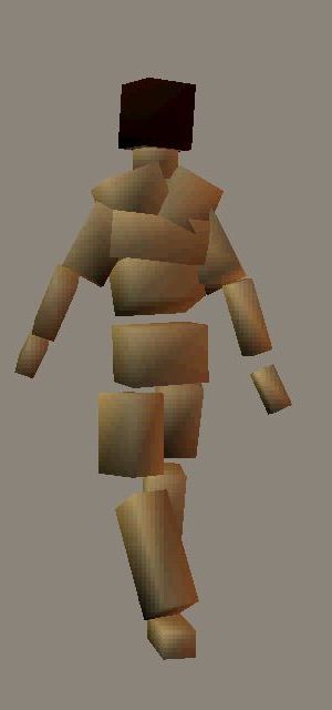
IEEE TRANSACTIONS ON PATTERN ANALYSIS AND MACHINE INTELLIGENCE. SUBMITTED FOR REVIEW.                                                           5

                                                                                                                         a

                     RVM Training Algorithm                                                                 0

     1)   Initialize A with ridge regression. Initialize the run-
          ning scale estimates ascale = kak for the components                                             –1

          or vectors a.
     2)   Approximate the ν log kak penalty terms with
                                                                                                           –2
          “quadratic bridges”, the gradients of which match
          at ascale . I.e. the penalty terms take the form
          ν             2
           2 (a/ascale ) + const.                                                                          –3
          (One can set const = ν(logkascale k − 12 ) to match the
          function values at ascale , but this value is irrelevant for
          the least squares minimization.)                                                                 –4

     3)   Solve the resulting linear least squares problem in A.         Fig. 5. “Quadratic bridge” approximations to the ν log kak regularizers.
     4)   Remove any components a that have become zero,                 These are introduced to prevent parameters from prematurely becoming
                                                                         trapped at zero. (See text.)
          update the scale estimates ascale = kak, and continue
          from 2 until convergence.
                                                                                                                     P
Fig. 4.   An outline of our RVM training algorithm.                      of y, and columnwise ones, R(A) = ν k log kak k where
                                                                         ak is the k th column of A, which select a common set of
                                                                         relevant basis functions for all components of y. Both priors
scale hyperparameter. Integrating out the hyperpriors (which             give similar results, but one of the main advantages of sparsity
can be done analytically) gives singular, highly nonconvex               is in reducing the number of basis functions (support features
total priors of the form p(a) ∼ kak−ν for each parameter or              or examples) that need to be evaluated, so in the experiments
parameter group a, where ν is a hyperprior parameter. Taking             shown we use columnwise priors. Hence, we minimize
log likelihoods gives an equivalent regularization penalty of
the form R(a) = ν log kak. Note the effect of this penalty.                                                     X
If kak is large, the ‘regularizing force’ dR/da ∼ ν/kak                                    kA F − Yk2 + ν            log kak k               (5)
is small so the prior has little effect on a. But the smaller                                                    k
kak becomes, the greater the regularizing force becomes.
At a certain point, the data term no longer suffices to hold
the parameter at a nonzero value against this force, and the             C. Choice of Basis
parameter rapidly converges to zero. Hence, the fitted model is             We tested two kinds of regression bases f (x). (i) Lin-
sparse — the RVM automatically selects a subset of ‘relevant’            ear bases, f (x) ≡ x, simply return the input vector, so
basis functions that suffices to describe the problem. The               the regressor is linear in x and the RVM selects rele-
regularizing effect is invariant to rescalings of f () or Y. (E.g.       vant features (components of x). (ii) Kernel bases, f (x) =
                                                                                                     >
scaling f → αf forces a rescaling A → A/α with no change                 (K(x, x1 ) · · · K(x, xn )) , are based on a kernel function
in residual error, so the regularization forces 1/kak ∝ α                K(x, xi ) instantiated at training examples xi , so the RVM
track the data-term gradient A F F> ∝ α correctly). ν serves             effectively selects relevant examples. Our experiments with
both as a sparsity parameter and as a scale-free regularization          various kernels and combinations of kernels and linear func-
parameter. The complete RVM model is highly nonconvex                    tions show that kernelization (of our already highly non linear
with many local minima and optimizing it can be problematic              features) gives a small but useful improvement in performance
because relevant parameters can easily become accidentally               — about 0.8◦ per body angle, out of a total mean error
‘trapped’ in the singularity at zero. However, in practice this          of around 7◦ . The form and parameters of the kernel have
does not prevent RVMs from giving useful results. Setting ν to           remarkably little influence. The experiments shown use a
                                                                                                                    2
optimize the estimation error on a validation set, one typically         Gaussian kernel K(x, xi ) = e−βkx−xi k with β estimated
finds that RVMs give sparse regressors with performance very             from the scatter matrix of the training data, but other β values
similar to the much denser ones from analogous methods with              within a factor of 2 from this value give very similar results.
milder priors.
   To train our RVMs, we do not use Tipping’s algorithm                                  IV. P OSE FROM S TATIC I MAGES
[29], but rather a continuation method based on succes-
sively approximating the ν log kak regularizers with quadratic              We conducted experiments using a database of motion
“bridges” ν (kak/ascale )2 chosen to match the prior gradient at         capture data for a 54 d.o.f. body model (3 angles for each
ascale , a running scale estimate for a (see fig. 5). The bridging       of 18 joints, including body orientation w.r.t the camera). We
changes the apparent curvature if the cost surfaces, allowing            report mean (over all 54 angles) RMS absolute difference
parameters to pass through zero if they need to, with less risk          errors between the true and estimated joint angle vectors, in
of premature trapping. The algorithm is sketched in figure 4.            degrees:
   We have tested both componentwise priors, R(A) =                                               1 X
                                                                                                      m
                                                                                    D(x, x0 ) =         |(xi − x0i ) mod ± 180◦ |
  P
ν jk log |Ajk |, which effectively allow a different set of                                                                                  (6)
                                                                                                  m i=1
relevant basis functions to be selected for each dimension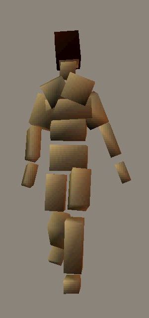
IEEE TRANSACTIONS ON PATTERN ANALYSIS AND MACHINE INTELLIGENCE. SUBMITTED FOR REVIEW.                                                                                                           6

                                 15
                                                                                   Complete Body
                                 14                                                Torso
                                                                                   Right Arm

           Mean error (in degrees)
                                 13                                                Left Leg

                                 12

                                 11

                                 10

                                     9

                                     8

                                     7

                                     6
                                      2         2.5   3     3.5     4      4.5     5     5.5       6
                                                                  log ν

Fig. 6. Mean test-set fitting error for different combinations of body parts,                                                                                   LSR     RVM      SVM
versus the linear RVM spareseness parameter ν. The minima indicate the                                                       Average error (in degrees)         5.95    6.02     5.91
optimal sparsity / regularization settings for each body part. Limb regressors                                               % of support vectors retained      100      6        53
are sparser than body or torso ones: the whole body regressor retains 23
features; torso, 31; right arm, 10; and the left leg, 7.
                                                                                                                   Fig. 8. (Top) A summary of our various regressors’ performance on different
                                                                                                                   combinations of body parts for the spiral walking test sequence. (Bottom) Error
                                                                                                                   measures for the full body using Gaussian kernel bases with the corresponding
                                                                                                                   number of support vectors retained.

                                                                                                                   flexible modelling of the relationship between x and z, but
                                                                                                                   reveals which of the original input features encode useful pose
                                                                                                                   information, as the RVM directly selects relevant components
     (a)                                  (b)             (c)             (d)           (e)            (f)         of z.
                                                                                                                      One might expect that, e.g. the pose of the arms was mainly
Fig. 7. Silhouette points whose shape context classes are retained by the                                          encoded by (shape-context classes receiving contributions
RVM for regression on (a) left arm angles, (b) right leg angles, shown on a                                        from) features on the arms, and so forth, so that the arms
sample silhouette. (c-f): Silhouette points encoding torso & neck parameter
values over different view points and poses. On average, about 10 features
                                                                                                                   could be regressed from fewer features than the whole body,
covering about 10% of the silhouette suffice to estimate the pose of each body                                     and could be regressed robustly even if the legs were occluded.
part.                                                                                                              To test this, we divided the body joints into five subsets —
                                                                                                                   torso & neck, the two arms, and the two legs — and trained
                                                                                                                   separate linear RVM regressors for each subset. Fig. 6 shows
The training silhouettes were created by using P OSER to render                                                    that similar validation-set errors are attained for each part, but
the motion captured poses, and reduced to 100-D histograms                                                         the optimal regularization level is significantly smaller (there
by vector quantizing their shape context distributions using                                                       is less sparsity) for the torso than for the other parts. Fig. 7
centres selected by k-means.                                                                                       shows the silhouette points whose contexts contribute to the
   We compare here results of regressing body pose x (after                                                        features (histogram classes) that were selected as relevant,
transforming from 54-D to 55-D as described in section II-B)                                                       for several parts and poses. The two main observations are
on the silhouette descriptors z using ridge, RVM and SVM                                                           that the regressors are indeed sparse — only about 10 of the
[32] based regression methods on linear and kernel bases with                                                      100 histogram bins were classed as relevant on average, and
the functional form given in section III:                                                                          the points contributing to these tend to be well localized in
                                                                        p
                                                                        X                                          important-looking regions of the silhouette — but that there
                         x = A f (z) +  ≡                                      ak φk (z) +                 (7)   is a good deal of non-locality between the points selected for
                                                                        k=1                                        making observations and the parts of the body being estimated.
Ridge regression and RVM regression use quadratic loss                                                             This nonlocality is somewhat surprising. It is perhaps only
functions to measure x-space prediction errors, as described                                                       due to the extent to which the motions of different body
in section III, while SVM regression uses the -insensitive                                                        segments are synchronized during natural walking motion, but
loss function [26] and a linear programming method for                                                             if it turns out to be true for larger training sets containing
training. The results shown here use the SVM-light [15] for                                                        less orchestrated motions, it may suggest that the localized
implementation.                                                                                                    calculations of model-based pose recovery actually miss a
                                                                                                                   good deal of the information most relevant for pose.
A. Implicit Feature Selection
  Kernel based RVM regression gives reliable pose estimates                                                        B. Performance Analysis
while retaining only about 6% of the training examples, but                                                          Fig. 8 summarizes the test-set performance of the various
working in kernel space hides information associated with                                                          regression methods studied — kernelized and linear basis
individual input features (components of z-vectors). Con-                                                          versions of damped least squares regression (LSR), RVM and
versely, linear-basis RVM regression (f (z) = z) provides less                                                     SVM regression, for the full body model and various subsets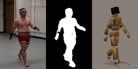
IEEE TRANSACTIONS ON PATTERN ANALYSIS AND MACHINE INTELLIGENCE. SUBMITTED FOR REVIEW.                                                              7

                                                                                  possible poses. As one diagnostic for this, recall that to allow
                                                                                  for the 360◦ wrap around of the heading angle θ, we actually
                                                                                  regress (a, b) = (cos θ, sin θ) rather than θ. In ambiguous
                                                                                  cases, the regressor tends to compromise between several
                                                                                  possible solutions, and hence returns an (a, b) vector whose
                                                                                  norm is significantly less than one. These events are strongly
                                                                                  correlated with large estimation errors in θ, as illustrated in
                                                                                  fig. 10.
                                                                                     Fig. 11 shows reconstruction results on some real images.
                                                                                  The reconstruction quality demonstrates the method’s robust-
                                                                                  ness to imperfect visual features, as a quite naive background
                                                                                  subtraction method was used to extract somewhat imperfect
                                                                                  body silhouettes from these images. The last example demon-
     (a)          (b)          (c)          (d)          (e)          (f)         strates the problem of silhouette ambiguity: the method returns
                                                                                  a pose with the left knee bent instead of the right one as the
Fig. 9. Some sample pose reconstructions for a spiral walking sequence            silhouette looks the same in the two cases, causing a glitch in
not included in the training data. The reconstructions were computed with a
Gaussian kernel RVM, using only 156 of the 2636 training examples. The
                                                                                  the output pose.
mean angular error per d.o.f. over the whole sequence is 6.0◦ . While (a-            Although numerically our results are already significantly
c) show accurate reconstructions, (d-f) are examples of misestimation: (d)        better than others presented in the literature (6◦ as compared
illustrates a label confusion (the left and right legs have been interchanged),
(e,f) are examples of compromised solutions where the regressor has averaged
                                                                                  to RMS errors of about 20◦ per d.o.f. reported in [22]), our
between two or more distinct possibilities. Using single images alone, we find    pose reconstructions do still contain a significant amount of
∼ 15% of our results are misestimated.                                            temporal jitter, and also occasional glitches. The jitter is to be
                                                                                  expected given that each image is processed independently.
                                                                                  It can be reduced by temporal filtering (simple smoothing or
of it — at optimal regularizer settings computed using 2-fold                     Kalman filtering), and also by adding a temporal dimension
cross validation. All output parameters are normalized to have                    to the regressor. The glitches occur when more than one
unit variance before regression and the tube width  in the                       solution is possible, causing the regressor to either ‘select’ the
SVM is set to correspond to an error of 1◦ for each joint                         wrong solution, or to output a compromised solution, different
angle. Kernelization brings only a small advantage (0.8◦ on an                    from each. One possible way to reduce such errors would be
average) over purely linear regression against our (highly non-                   to incorporate stronger features such as internal body edges
linear) descriptor set. The regressors are all found to give their                within the silhouette, however the problem is bound to persist
best results at similar optimal kernel parameters, which are                      as important internal body edges are often not visible and
more or less independent of the regularization prior strengths.                   useful body edges have to be distinguished from irrelevant
The RVM regression gives very slightly higher errors than the                     clothing texture edges. Furthermore, even without these limb
other two regressors, but much more sparsity. For example,                        labelling ambiguities, depth related ambiguities continue to
in our whole-body method, the final RVM selects just 156                          remain an issue. By relying on experimentally observed poses,
(about 6%) of the 2636 training points as basis kernels, to                       our single image method has already reduced this ambiguity
give a mean test-set error of 6.0◦ . We attribute the slightly                    significantly, but human beings often rely on very subtle cues
better performance of the SVM to the different form of its loss                   to disambiguate multiple solutions.
function. The overall similarity of the results obtained from                        In the absence of multiple simultaneous views, temporal
the 3 different regressors confirms that our representation and                   continuity is an important supplementary source of informa-
framework are insensitive to the exact method of regression                       tion for resolving these ambiguities. In the following two
used.                                                                             sections, we describe two different approaches that exploit
   Fig. 9 shows some sample pose estimation results, on                           continuity within our regression model.
silhouettes from a spiral-walking motion capture sequence that
was not included in the training set. The mean estimation                                        V. T RACKING AND R EGRESSION
error over all joints for the Gaussian RVM in this test is                           This section describes a novel ‘discriminative’ tracking
6.0◦ , but the error for individual joints varies depending on                    framework that fuses pose predictions from a learned dynam-
the range and discernibility of each joint angle. The RMS                         ical model into our single image regression framework, to
errors obtained for some key body angles are as follows (the                      correctly reconstruct the most likely 3D pose at each time step.
ranges of variation of these angles in the test set are given                     The 3D pose can only be observed indirectly via ambiguous
in parentheses): body heading angle: 17◦ (360◦ ), left shoulder                   and noisy image measurements, so it is appropriate to start
angle: 7.5◦ (50.8◦ ), and right hip angle: 4.2◦ (47.4◦ ). Fig. 10                 by considering the Bayesian tracking framework in which our
(top) plots the estimated and actual values of the overall body                   knowledge about the state (pose) xt given the observations
heading angle θ during the test sequence, showing that much                       up to time t is represented by a probability distribution, the
of the error is due to occasional large errors that we will refer                 posterior state density p(xt | zt , zt−1 , . . . , z0 ).
to as “glitches”. These are associated with ambiguous cases                          Given an image observation zt and a prior p(xt ) on the
where the silhouette might easily arise from any of several                       corresponding pose xt , the posterior likelihood for xt is usu-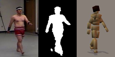
IEEE TRANSACTIONS ON PATTERN ANALYSIS AND MACHINE INTELLIGENCE. SUBMITTED FOR REVIEW. 8
250
200
Estimated angle where p(zt |xt ) is an explicit ‘generative’ observation model
Actual angle
that predicts zt and its uncertainty given xt . Unfortunately,
Torso angle (in degrees)
150
100 when tracking objects as complicated as the human body,
50 the observations depend on a great many factors that are
0 difficult to control, ranging from lighting and background to
−50 body shape and clothing style and texture, so any hand-built
−100 observation model is necessarily a gross oversimplification.
−150
One way around this would be to learn the generative model
−200
0 50 100 150 200 250 300 350 400 p(z|x) from examples, then to work backwards via its Jacobian
Time
100
to get a linearized state update, as in the extended Kalman
Torso angle error
filter. However, this approach is somewhat indirect, and it may
50
waste a considerable amount of effort modelling appearance
details that are irrelevant for predicting pose. Instead, we prefer
0 to learn a ‘diagnostic’ (discriminative or regressive) model
0 50 100 150 200 250 300 350 400
Time p(x|z) for the pose x given the observations z — c.f . the
Norm of angle vector
1
difference between generative and discriminative classifiers,
and the regression based trackers of [16, 33]. Similarly, in the
0.5 context of maximum likelihood pose estimation, we prefer to
learn a diagnostic regressor x = x(z), i.e. a point estimator
0
0 50 100 150 200
Time
250 300 350 400 for the most likely state x given the observations z, not a
generative predictor z = z(x). Unfortunately, this brings up
a second problem. As we have seen in the previous section,
Fig. 10. (Top): The estimated body heading (azimuth θ) over 418 frames of
the spiral walking test sequence, compared with its actual value from motion image projection suppresses most of the depth (camera-object
capture. (Middle, Bottom): Episodes of high estimation error are strongly distance) information and using silhouettes as image obser-
correlated with periods when the norm of the (cos θ, sin θ) vector that was vations induces further ambiguities owing to the lack of limb
regressed to estimate θ becomes small. These occur when similar silhouettes
arise from very different poses, so that the regressor is forced into outputing labelling. So the state-to-observation mapping is always many-
a compromise solution. to-one. These ambiguities make learning to regress x from z
difficult because the true mapping is actually multi-valued.
A single-valued least squares regressor tends to either zig-
zag erratically between different training poses, or (if highly
damped) to reproduce their arithmetic mean [7], neither of
which is desirable.
To reduce the ambiguity, we work incrementally from the
previous few states4 xt−1 , . . . (e.g. as was done in [10]). We
adopt the working hypothesis that given a dynamics based
estimate xt (xt−1 , . . .) — or any other rough initial estimate
x̌t for xt — it will usually be the case that only one of the
observation-based estimates is at all likely a posteriori. Thus,
we can use the x̌t value to “select the correct solution” for the
observation-based reconstruction xt (zt ). Formally this gives a
regressor xt = xt (zt , x̌t ), where x̌t serves mainly as a key
to select which branch of the pose-from-observation space to
use, not as a useful prediction of xt in its own right. To work
like this, the regressor must be well-localized in x̌t , and hence
nonlinear. Taking this one step further, if x̌t is actually a useful
estimate of xt (e.g. from a dynamical model), we can use a
single regressor of the same form, xt = xt (zt , x̌t ), but now
with a stronger dependence on x̌t , to capture the net effect of
implicitly reconstructing an observation-estimate xt (zt ) and
Fig. 11. 3D poses reconstructed from some real test images using a single
then fusing it with x̌t to get a better estimate of xt .
image for each reconstruction (the images are part of a sequence from
www.nada.kth.se/∼hedvig/data.html). The middle and lower rows respectively A. Learning the Regression Models
show the estimates from the original viewpoint and from a new one. The
first two columns show accurate reconstructions. In the third column, a noisy Our discriminative tracking framework now has two levels
silhouette causes slight misestimation of the lower right leg, while the final of regression. We formulate the models as follows and con-
column demonstrates a case of left-right ambiguity in the silhouette. tinue to use the methods described in section III:
4 As an alternative we tried regressing the pose x against a sequence of the
t
last few silhouettes (zt , zt−1 , . . .), but the ambiguities are found to persist
ally evaluated using Bayes’ rule, p(xt |zt ) ∝ p(zt |xt ) p(xt ), for several frames.
IEEE TRANSACTIONS ON PATTERN ANALYSIS AND MACHINE INTELLIGENCE. SUBMITTED FOR REVIEW.                                                                                                 9

                                                                                                                    30                      Tracking results for left hip angle
   1) Dynamical (Prediction) Model: Human body dynam-                                                                                       True value of this angle
                                                                                                                    20
ics can be modelled fairly accurately with a second order

                                                                                     Left hip angle (in degrees)
                                                                                                                    10
linear autoregressive process, xt = x̌t + , where x̌t ≡
                                                                                                                     0
à xt−1 + B̃ xt−2 is the second order dynamical estimate of
                                                                                                              −10
xt and  is a residual error vector (c.f . e.g. [3]). To ensure
                                                                                                              −20
dynamical stability and avoid over-fitting, we actually learn
                                                                                                              −30
the autoregression for x̌t in the following form:
                                                                                                              −40

           x̌t ≡ (I + A)(2xt−1 − xt−2 ) + B xt−1                   (8)                                        −50
                                                                                                                         0   50     100    150       200        250       300
where I is the m × m identity matrix. This form helps                                                                                      Time
                                                                                                                    0
to maintain stability by converging towards a default linear
prediction if A and B are overdamped. We estimate A and B                                                          20

by regularized least squares regression against xt , minimizing                                                    40

                                                                                     Kernel bases
kk22 + λ(kAk2Frob + kBk2Frob ) over the training set, with the
regularization parameter λ set by cross-validation to give a                                                       60

well-damped solution with good generalization.
                                                                                                                   80
    2) Likelihood (Correction) Model: Now consider the ob-
servation model. As discussed above, the underlying density                                                   100

p(xt | zt ) is highly multimodal owing to the pervasive am-                                                          0       50     100    150       200        250       300
biguities in reconstructing 3D pose from monocular images,                                                                                 Time

so no single-valued regression function xt = xt (zt ) can
give acceptable point estimates for xt . However much of the              Fig. 12. An example of mistracking caused by an over-narrow pose kernel
‘glitchiness’ and jitter observed in the static reconstructions of        Kx . The kernel width is set to 1/10 of the optimal value, causing the tracker
                                                                          to lose track from about t=120, after which the state estimate drifts away
section IV-B can be removed by feeding x̌t into the regression            from the training region and all kernels stop firing by about t=200. Left: the
model. The combined regressor can be formulated in several                variation of a left hip angle parameter for a test sequence of a person walking
different ways. The simplest is to linearly combine x̌t with              in a spiral. Right: The temporal activity of the 120 kernels (training examples)
                                                                          during this track. The banded pattern occurs because the kernels are samples
the estimate xt given by equation (7), but this only smooths              taken from along a similar 2.5 cycle spiral walking sequence, each circuit
the results, reducing jitter, while still continuing to give wrong        involving about 8 steps. The similarity between adjacent steps and between
solutions when (7) returns a wrong estimate. We thus include              different circuits is clearly visible, showing that the regressor can locally still
                                                                          generalize well.
a non-linear dependence on x̌t with zt in the observation-
based regressor, giving a state sensitive observation update.
                                                                                                                   5.5
Our full regression model also includes an explicit linear x̌t
term to represent the direct contribution of the dynamics to the
                                                                                     RMS error

                                                                                                                    5
overall state estimate, so the final model becomes xt ≡ x̂t +0
where 0 is a residual error to be minimized, and:                                                                 4.5
                  p
                X                                       x̌t                                                        4
  x̂t = C x̌t +      dk φk (x̌t , zt ) ≡ C D                        (9)                                             0.7      0.75    0.8    0.85        0.9       0.95            1
                                                     f (x̌t , zt )                                                                   Damping factor (s)
                k=1

Here, {φk (x, z) | k = 1 . . . p} is a set of scalar-valued non-
                                                                          Fig. 13. The variation of the RMS test-set tracking error with damping factor
linear basis functions for the regression, and dk are the                 s. See the text for discussion.
corresponding Rm -valued weight vectors. For compactness,
we gather these into an Rp -valued feature vector f (x, z) ≡
                              >
(φ1 (x, z), . . . , φp (x, z)) and an m×p weight matrix D ≡
                                                                          the method tends to average over (or zig-zag between) several
(d1 , . . . , dp ). In the experiments reported here, we used
                                                                          alternative pose-from-observation solutions, which defeats the
instantiated-kernel bases of the form
                                                                          purpose of including x̌ in the observation regression. On the
                φk (x, z) = Kx (x, xk ) · Kz (z, zk )             (10)    other hand, too much locality in x effectively ‘switches off’
                                                                          the observation-based state corrections whenever the estimated
where (xk , zk ) is a training example and Kx , Kz are (here,
                                                                          state happens to wander too far from the observed training
independent Gaussian) kernels on x-space and z-space,
                             2                               2            examples xk . So if the x-kernel is set too narrow, observation
Kx (x, xk ) = e−βx kx−xk k and Kz (z, zk ) = e−βz kz−zk k .
                                                                          information is only incorporated sporadically and mistracking
Building the basis from Gaussians based at training examples
                                                                          can easily occur. Fig. 12 illustrates this effect, for an x-kernel
in joint (x, z) space makes examples relevant only if they have
                                                                          a factor of 10 narrower than the optimum. The method initially
similar image silhouettes and similar underlying poses.
                                                                          seemed to be sensitive to the kernel width parameters, but after
Mistracking due to extinction. Kernelization in joint (x, z)              fixing good default values by cross-validation on an indepen-
space allows the relevant branch of the inverse solution to               dent motion sequence we observed accurate performance over
be chosen, but it is essential to choose the relative widths of           a sufficiently wide range for both the kernel widths: a tolerance
the kernels appropriately. If the x-kernel is chosen too wide,            factor of about 2 on βx and about 4 on βz .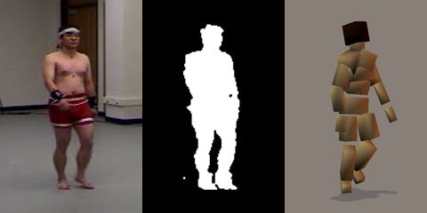
IEEE TRANSACTIONS ON PATTERN ANALYSIS AND MACHINE INTELLIGENCE. SUBMITTED FOR REVIEW.                                                          10

Neutral vs Damped Dynamics. The coefficient matrix C
in (9) plays an interesting role. Setting C ≡ I forces the
correction model to act as a differential update on x̌t (what
we refer to as having a ‘neutral’ dynamical model). On the
other extreme, C ≡ 0 gives largely observation-based state
estimates with only a latent dependence on the dynamics. An
intermediate setting, however, turns out to give the best overall
results. Damping the dynamics slightly ensures stability and
controls drift — in particular, preventing the observations from
disastrously ‘switching off’ because the state has drifted too far
from the training examples — while still allowing a reasonable
amount of dynamical smoothing. Usually we estimate the full
(regularized) matrix C from the training data, but to get an
                                                                            t=001       t=060      t=120       t=180       t=240      t=300
idea of the trade-offs involved, we also studied the effect of
explicitly setting C = sI for s ∈ [0, 1]. We find that a small
                                                                     Fig. 15. Sample pose reconstructions for the spiral walking sequence using
amount of damping, sopt ≈ .98 gives the best results overall,        the tracking method. This sequence was not included in the training data, and
maintaining a good lock on the observations without losing too       corresponds to figures 14(c) & (f). The reconstructions were computed with a
much dynamical smoothing (see fig. 13.) This simple heuristic        Gaussian kernel RVM, using only 18% training examples. The average RMS
                                                                     estimation error per d.o.f. over the whole sequence is 4.1◦ .
setting gives very similar results to the model obtained by
learning the full matrix C.
                                                                     a special case of (9) where C = 0 and Kx = 1. Panels
B. Tracking Results                                                  (c),(f) show that jointly regressing dynamics and observations
                                                                     gives a significant improvement in estimation quality, with
   We trained the new regression model (9) on our motion
                                                                     smoother and stabler tracking. There is still some residual
capture data as in section IV. For these experiments, we used
                                                                     misestimation of the hip angle in (c) at around t=140 and
8 different sequences totalling about 2000 instantaneous poses
                                                                     t=380. At these points, the subject is walking directly towards
for training, and another two sequences of about 400 points
                                                                     the camera (heading angle θ∼0◦ ), so the only cue for hip angle
each as validation and test sets. Errors are again reported as
                                                                     is the position of the corresponding foot, which is sometimes
described by (6).
                                                                     occluded by the opposite leg. Humans also find it difficult to
   The dynamical model is learned from the training data ex-
                                                                     estimate this angle from the silhouette at these points.
actly as described in §V-A.1, but when training the observation
                                                                        Fig. 15 shows some silhouettes and corresponding maxi-
model, we find that its coverage and capture radius can be
                                                                     mum likelihood pose reconstructions, for the same test se-
increased by including a wider selection of x̌t values than
                                                                     quence. The 3D poses for the first two time steps were set by
those produced by the dynamical predictions. Hence, we train
                                                                     hand to initialize the dynamical predictions. The average RMS
the model x = xt (x̌, z) using a combination of ‘observed’
                                                                     estimation error over all joints using the RVM regressor in this
samples (x̌t , zt ) (with x̌t computed from (8)) and artificial
                                                                     test is 4.1◦ . Well-regularized least squares regression over the
samples generated by Gaussian sampling N (xt , Σ) around the
                                                                     same basis gives similar errors, but has much higher storage
training state xt . The observation zt corresponding to xt is
                                                                     requirements. The Gaussian RVM gives a sparse regressor for
still used, forcing the observation based part of the regressor
                                                                     (9) involving only 348 of the 1927 (18%) training examples,
to rely mainly on the observations, i.e. on recovering xt (or
                                                                     thus allowing a significant reduction in the amount of training
at least an update to x̌t ) from zt , using x̌t mainly as a hint
                                                                     data that needs to be stored. The reconstruction results on two
about the inverse solution to choose. The covariance matrix Σ
                                                                     test video sequences are shown in figs 16 and 19.
is chosen to reflect the local scatter of the training examples,
                                                                        In terms of computation time, the final RVM regressor
with a larger variance along the tangent to the trajectory at
                                                                     already runs in real time in Matlab. Silhouette extraction
each point to ensure that phase lag between the state estimate
                                                                     and shape-context descriptor computations are currently done
and the true state is reliably detected and corrected.
                                                                     offline, but should be feasible online in real time. The offline
   Fig. 14 illustrates the relative contributions of the dynamics
                                                                     learning process takes about 2-3 min for the RVM with ∼2000
and observation terms in our model by plotting tracking results
                                                                     data points, and currently about 20 min for Shape Context ex-
for a motion capture test sequence in which the subject
                                                                     traction and clustering (this being highly unoptimized Matlab
walks in a decreasing spiral. This sequence was not included
                                                                     code).
in the training set, although similar ones were. The purely
dynamical model (8) provides good estimates for a few time           Automatic Initialization: The method is reasonably robust
steps, but gradually damps and drifts out of phase. Such             to initialization errors. Although the results shown in figs. 14
damped oscillations are characteristic of second order linear        and 15 were obtained by initializing from ground truth, we
autoregressive dynamics, trained with enough regularization to       also tested the effects of automatic (and hence potentially
ensure model stability. The results based on observations alone      incorrect) initialization. In an experiment in which the tracker
without any temporal information are included again here for         was automatically initialized at each time step in turn using
comparison. These are obtained from (7), which is actually           the pure observation model, then tracked forwards and back-
IEEE TRANSACTIONS ON PATTERN ANALYSIS AND MACHINE INTELLIGENCE. SUBMITTED FOR REVIEW. 11
(a) Pure dynamical model on test set (d) Pure dynamical model on test set
30 250
Tracking results for left hip angle Tracking results for torso angle
True value of this angle True value of this angle
Torso heading angle (in degrees)
200
20
Left hip angle (in degrees)
150
10
100
0 50
−10 0
−50
−20
−100
−30
−150
−40 −200
0 50 100 150 200 250 300 350 400 0 50 100 150 200 250 300 350 400
Time Time
(b) Pure observation model on test set (e) Pure observation model on test set
30 250
Tracking results for left hip angle Tracking results for torso angle
True value of this angle True value of this angle
Torso heading angle (in degrees)
200
20
Left hip angle (in degrees)
150
10
100
0 50
−10 0
−50
−20
−100
−30
−150
−40 −200
0 50 100 150 200 250 300 350 400 0 50 100 150 200 250 300 350 400
Time Time
(c) Joint regression model on test set (f) Joint regression model on test set
30 250
Tracking results for left hip angle Tracking results for torso angle
True value of this angle Torso heading angle (in degrees) 200 True value of this angle
20
Left hip angle (in degrees)
150
10
100
0 50
−10 0
−50
−20
−100
−30
−150
−40 −200
0 50 100 150 200 250 300 350 400 0 50 100 150 200 250 300 350 400
Time Time
Fig. 14. Sample tracking results on a spiral walking test sequence. (a) Variation of the left hip-angle parameter, as predicted by a pure dynamical model
initialized at t = {0, 1}, (b) Estimated values of this angle from regression on observations alone (i.e. no initialization or temporal information), (c) Results
from our novel joint regressor, obtained by combining dynamical and state+observation based regression models. (d,e,f) Similar plots for the overall body
rotation angle. Note that this angle wraps around at 360◦ , i.e. θ ' θ ± 360◦ .
wards using the dynamical tracker, the initialization lead to one type in nature. Firstly, there exist instances where any
successful tracking in 84% of the cases. The failures were 3D pose in a continuous range seems to explain the given
the ‘glitches’, where the observation model gave completely silhouette observation quite well, e.g. estimating out-of-plane
incorrect initializations. rotations where the limb length signal is not strong enough to
estimate the angle accurately. Here one would desire a broad
VI. R ESOLVING A MBIGUITIES USING A M IXTURE OF
distribution in 3D pose space as the output from a single
E XPERTS
silhouette. Other cases of ambiguity arise due to kinematic
In this section, we discuss an alternative approach to dealing flipping (c.f . [24]) or label-ambiguities (disambiguating the
with multiple possible solutions in the 3D pose estimation left and right arms/legs). In such cases, there is typically
problem. We extend our single image regression framework a finite discrete set of probable solutions — often only 2
from section IV to a mixture of regressors (often known as a or 4, but sometimes more. To deal with both of the above
mixture of experts [14]). Such a model enables the regressor to cases, we model the conditional density p(x|z) as a mixture
output more than one possible solution from a single silhouette of Gaussians:
— in general a multimodal probability density p(x|z). We
describe the formulation of our mixture model and show how
K
it can be used in a multiple hypothesis probabilistic tracking X
p(x|z) = πk N (x̄k , Λk ) (11)
framework to achieve smooth reconstruction tracks free from
k=1
glitches.
where x̄k is computed by learning a regressor x̄k = Ak f (z)+
A. Probabilistic pose from static images bk within each mixture component, and Λk (a diagonal
A close analysis of the nature of ambiguities in the covariance matrix in our case) is estimated from residual
silhouette-to-pose problem indicates that they are of more than errors. πk are the gating probabilities of the regressors. SettingYou can also read