Driver Glance Classification In-the-wild: Towards Generalization Across Domains and Subjects
←
→
Page content transcription
If your browser does not render page correctly, please read the page content below
Driver Glance Classification In-the-wild: Towards Generalization Across
                                                                        Domains and Subjects*

                                                       Sandipan Banerjee1 , Ajjen Joshi1 , Jay Turcot1 , Bryan Reimer2 , and Taniya Mishra*3
                                                                                                  1
                                                                                                   Affectiva, USA
                                                                                  2
                                                                                      Massachusetts Institute of Technology, USA
                                                                                                 3
                                                                                                   SureStart, USA
arXiv:2012.02906v2 [cs.CV] 20 Jan 2021

                                                                     {sandipan.banerjee, ajjen.joshi, jay.turcot}@affectiva.com
                                                                                          {reimer}@mit.edu
                                                                                      {taniya.mishra}@mysurestart.com

                                                                       Abstract
                                             Distracted drivers are dangerous drivers. Equipping ad-
                                         vanced driver assistance systems (ADAS) with the ability to
                                         detect driver distraction can help prevent accidents and im-
                                         prove driver safety. In order to detect driver distraction, an
                                         ADAS must be able to monitor their visual attention. We
                                         propose a model that takes as input a patch of the driver’s
                                         face along with a crop of the eye-region and classifies their
                                         glance into 6 coarse regions-of-interest (ROIs) in the ve-
                                         hicle. We demonstrate that an hourglass network, trained
                                         with an additional reconstruction loss, allows the model to
                                         learn stronger contextual feature representations than a tra-
                                         ditional encoder-only classification module. To make the
                                         system robust to subject-specific variations in appearance
                                         and behavior, we design a personalized hourglass model                Figure 1: Our model takes as input the driver’s face and eye patch and
                                                                                                               generates glance predictions over 6 coarse regions-of-interest (ROIs): 1.
                                         tuned with an auxiliary input representing the driver’s base-
                                                                                                               Instrument Cluster, 2. Rearview Mirror, 3. Right, 4. Left, 5. Centerstack,
                                         line glance behavior. Finally, we present a weakly super-             6. Road. While requiring little labeled data, it can jointly predict the glance
                                         vised multi-domain training regimen that enables the hour-            ROI on samples from different domains (e.g. car interior) that vary in cam-
                                         glass to jointly learn representations from different domains         era type, angle and lighting. In the figure, both subjects are looking at the
                                                                                                               road, but appear different due to mismatch in camera angle and lighting.
                                         (varying in camera type, angle), utilizing unlabeled samples
                                         and thereby reducing annotation cost.
                                                                                                               also monitor driver attention to manage and motivate im-
                                                                                                               proved awareness [11]. For example, the system can decide
                                         1. Introduction
                                                                                                               whether a driver’s attention needs to be cued back to the
                                            Driver distraction has been shown to be a leading cause
                                                                                                               road prior to safely handing them back the control.
                                         of vehicular accidents [14]. Anything that competes for a
                                                                                                                  A real-time system that can classify driver attention into
                                         driver’s attention, such as talking or texting on the phone,
                                                                                                               a set of ROIs can be used to infer their overall attentiveness
                                         using the car’s navigation system or eating, can be a cause
                                                                                                               and offer predictive indication of attention failures associ-
                                         of distraction. A distracted individual often directs their vi-
                                                                                                               ated with crashes and near-crashes [55]. Real-time tracking
                                         sual attention away from driving, which has been shown
                                                                                                               of driver gaze from video is attractive because of the low
                                         to increase accident risk [34]. Therefore, driver glance be-
                                                                                                               equipment cost but challenging due to variations in illumi-
                                         havior can be an important signal in determining their level
                                                                                                               nation, eye occlusions caused by eyeglasses/sunglasses and
                                         of distraction. A system that can accurately detect where
                                                                                                               poor video quality due to vehicular movements and sensor
                                         the driver is looking can then be used to alert drivers when
                                                                                                               noise. In this paper, we propose a model that can predict
                                         their attention shifts away from the road. Such systems can
                                                                                                               driver glance ROI, given a patch of the driver’s face along
                                           * Work   done while at Affectiva                                    with a crop of their eye-region (Figure 1). We show that an

                                                                                                           1
hourglass network [51, 45], composed of encoder-decoder              they typically require user or session-specific calibration to
modules, trained with a reconstruction loss on top of the            achieve good performance. Appearance-based, calibration-
classification task, performs better than a vanilla CNN. The         free gaze estimation has numerous applications in com-
reconstruction task serves as a regularizer [44], helping the        puter vision, from gaze-based human-computer interaction
model learn robust representations of the input by implicitly        to analysis of visual behavior. Researchers have utilized
leveraging useful information around its context[50, 47].            both real [75] and synthetic data [71, 70] to model gaze
    However, a model that makes predictions based on only            behavior, with generative approaches used to bridge the
a single static frame may struggle to deal with variations           gap between synthetic and real distributions, so that mod-
in subject characteristics not well represented in the train-        els trained on one domain work well on another [58, 29].
ing set (e.g. a shorter or taller-than average driver may have           Glance Classification: In the case of driver distraction,
different appearances for the default on-the-road driving be-        classifying where the driver is looking from an estimated
havior). To address this challenge, we add an auxiliary input        gaze vector involves finding the intersection between the
stream representing the subject’s baseline glance behavior,          gaze vector and the 3D car geometry. A simpler alternative
yielding improved performance over a rigid network.                  is to directly classify the driver image into a set of car ROIs
    Another challenge associated with an end-to-end glance           using head pose [26], as well as eye region appearance[16].
classification system is the variation in camera type                Rangesh et al. focused on estimating driver gaze in the pres-
(RGB/NIR) and placement (on the steering wheel or                    ence of eye-occluding glasses to synthetically remove eye-
rearview mirror). Due to variations in cabin configuration,          glasses from input images before feeding them to a classi-
it is impossible to place the camera in the same location            fication network [49]. Ghosh et al. recently introduced the
with a consistent view of the car interior and the driver.           Driver Gaze in the Wild (DGW) dataset to further encour-
Therefore, a model trained on driver head-poses associ-              age research in this area [20].
ated with a specific camera-view may not generalize. To                  Personalization: Personalized training has been applied
overcome this domain-mismatch challenge, we present a                to other domains (e.g. facial action unit [10] and gesture
framework to jointly train models in the presence of data            recognition [72, 27]) but not yet on vehicular glance clas-
from multiple domains (camera types and views). Leverag-             sification. In the context of eye tracking, personalization
ing our backbone hourglass’ reconstruction objective, this           is usually achieved through apriori user calibration. [32] re-
framework can utilize unlabeled samples from multiple do-            ported results for unconstrained (calibration-free) eye track-
mains along with weak supervision to jointly learn stronger          ing from mobile devices and showed calibration to signifi-
domain-invariant representations for improved glance clas-           cantly improve performance. For personalizing gaze mod-
sification while effectively reducing labeling cost.                 els latent representation for each eye has been used [35], for
    In summary, we make the following contributions: (1)             utilizing saliency information in visual content [6] or adapt-
we propose an hourglass architecture that can predict driver         ing a generic example using a few training samples [74].
glance ROI from static images, illustrating the utility of
                                                                         Domain Invariance: Domain adaptation has been used
adding a reconstruction loss to learn more robust represen-
                                                                     in a variety of applications, e.g. object recognition [53]. Re-
tations even for classification tasks; (2) we design a per-
                                                                     searchers have trained shared networks with samples from
sonalized version of our hourglass model, that addition-
                                                                     different domains, regularized via an adaptation loss be-
ally learns residuals in feature space from the driver’s de-
                                                                     tween their embeddings [19, 64], or trained models with
fault ‘eyes-on-the-road’ behavior, to better tune output map-
                                                                     domain confusion to learn domain-agnostic embeddings
pings with respect to the subject’s default; (3) we formulate
                                                                     [65], implemented by reducing distance between the do-
a weakly supervised multi-domain training approach that
                                                                     main embeddings [63, 46] or reversing the gradient spe-
utilizes unlabeled samples for classification and allows for
                                                                     cific to domain classification during backpropagation [18].
model adaptation to novel camera types and angles, while
                                                                     Another popular approach towards domain adaptation is to
reducing the associated labeling cost.
                                                                     selectively fine-tune task specific models from pre-trained
                                                                     weights [24, 31] by freezing pre-trained weights that are
2. Related Work                                                      tuned to specific tasks or domains [38, 39] or selectively
   Computer-vision based driver monitoring systems [8]               pruning weights [4] to prudently adapt to new domains
have been used to estimate a driver’s state of fatigue [28],         [43]. Specific to head pose, lighting and expression agnostic
cognitive load [17] or whether the driver’s eyes are off the         face recognition, approaches like feature normalization us-
road [67].                                                           ing class centers [69, 76] and class separation using angular
   Gaze estimation: The problem of tracking gaze from                margins [36, 68, 12] have been proposed. Such recognition
video has been studied extensively [21, 5]. Professional             tasks have also benefitted from mixing samples from differ-
gaze tracking systems do exist (e.g. Tobii1 ), however               ent domains, like real and synthetic [40, 2].
   1 https://www.tobii.com/                                              While most research on gaze estimation proposes models

                                                                 2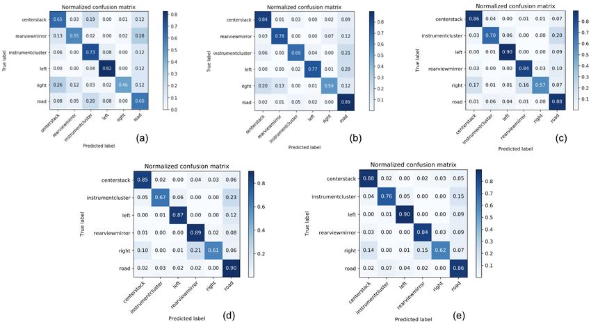
Figure 2: Sample frames from the datasets used in our experiments (MIT2013 (left), AVT (middle) and In-house (right). For each dataset, we present an
example raw frame captured by the camera, and an example each of a driver’s cropped face for each driver glance region-of-interest class.

that predict gaze vectors, our glance classification model di-               cle Technology (MIT-AVT) study was designed to collect
rectly predicts the actual ROI of the driver’s gaze inside the               large-scale naturalistic driving data for better understanding
vehicle. Unlike previous work, our multi-domain training                     of how drivers interact with modern cars to aid better design
approach tunes the model’s ROI prediction to jointly work                    and interfaces as vehicles transition into increasingly auto-
on multiple domains (e.g. car interiors), varying in camera                  mated systems. Each video in the AVT dataset was pro-
type, angle and lighting, while requiring very little labeled                cessed by a single coder with inter-rater reliability assess-
data. Our model can be personalized for continual tuning                     ments as detailed in [42].
based on the driver’s behavior and anatomy as well.                             In-house: This dataset was collected to train machine
                                                                             learning models to estimate gaze from the RGB and NIR
3. Dataset Description and Data Analysis                                     camera types and a challenging camera angle. A camera,
                                                                             with a wide-angle lens, was placed under the rear-view mir-
    MIT-2013: The dataset was extracted from a corpus of                     ror for this collection, the focus of which was to capture
driver-facing videos, which were collected as part of large                  data from a position where the entire cabin was visible.
driving study that took place on a local interstate high-                    Participants followed instructions from a protocol inside a
way [41]. For each participant in the study, videos of the                   static/parked car, where they glanced at various ROIs us-
drivers were collected either in a 2013 Chevrolet Equinox                    ing 3 behavior types: ‘owl’, ‘lizard’ and ‘natural’[16]. In
or a Volvo XC60. The participants performed a number of                      our experiments, we used samples from 85 participants - 50
tasks, such as using the voice interface to enter addresses or               for training, 18 for validation and 17 for testing. Videos of
combining it with manual controls to select phone numbers,                   each participant was manually annotated by 3 human label-
while driving. Frames with the frontal face of the drivers                   ers. Example frames from all three datasets are shown in
were then annotated to the following ROIs: ‘road’, ‘center                   Figure 2.
stack’, ‘instrument cluster’, ‘rearview mirror’, ‘left’, ‘right’,
‘left blindspot’, ‘right blindspot’, ‘passenger’, ‘uncodable’,               4. Proposed Models
and ‘other’. The data of interest was independently coded
by two evaluators and mediated according to standards de-                    4.1. Two-channel Hourglass
scribed by [60]. Following Fridman et al. [16], frames la-                       While a standalone classification (i.e. encoder with
beled ‘left’ and ‘left blindspot’ were given a single generic                prediction head) or reconstruction module (i.e. encoder-
‘left’ label and frames labeled ‘right’, ‘right blindspot’ and               decoder) can produce high performance numbers for recog-
‘passenger’ were given a generic ’right’ label, while frames                 nition or semantic segmentation or super-resolution tasks,
labeled ‘uncodable’, and ‘other’ were ignored. We used a                     combining them together has been shown to further boost
subset of the data with 97 unique subjects, which was split                  model performance [13, 37, 44, 22, 56]. The auxiliary
into 60 train, 17 validation and 20 test subjects.                           module’s (prediction or reconstruction) loss acts as a reg-
    AVT: This dataset contains driver-initiated, non-critical                ularizer [44] and boosts model performance on the primary
disengagement events of Tesla Autopilot in naturalistic                      task. For our specific task of driver glance classification,
driving [42] and was extracted from a large corpus of natu-                  adding a reconstruction element can tune the model weights
ralistic driving data, collected from an instrumented fleet of               to implicitly pay close attention to contextual pixels while
29 vehicles, each of which record the IMU, GPS, CAN mes-                     making a decision. Thus, instead of using a feed forward
sages, and video streams of the driver face, the vehicle cabin               neural network, as traditionally done for classification tasks
and the forward roadway [15]. The MIT Advanced Vehi-                         [33, 59, 23, 52], we use an hourglass structure consisting of

                                                                         3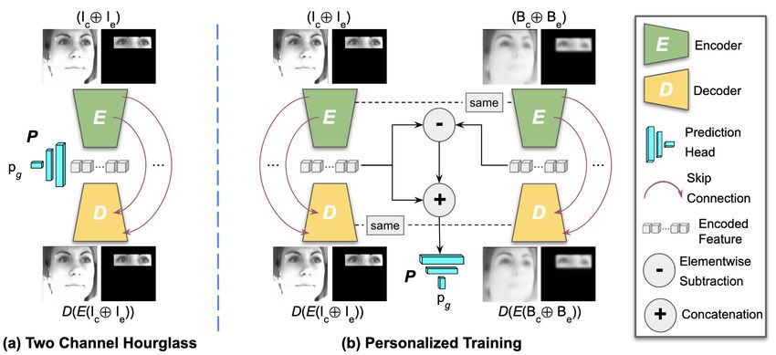
Figure 3: Illustration of our (a) two channel hourglass and (b) multi-stream personalization models described in Sections 4.1 and 4.2 respectively.

a pair of encoder (E) and decoder (D) modules [51].                              classes. The overall objective L is defined as:
   In our model, E takes as input the cropped face and
eye patch images Ic and Ie respectively, concatenated to-                                                  L = Lcls + λ1 Lrec                             (3)
gether as a two-channel tensor (Ic ⊕ Ie ) and produces a fea-
ture vector (i.e. E(Ic ⊕ Ie )) as its encoded representation.                    4.2. Personalized Training
This feature vector is then passed through a prediction head                         As mentioned earlier, introducing an auxiliary channel
P to extract the estimated glance vector pg , before being                       of baseline information can better tune the classification
sent to D to generate the face and eye patch reconstructions                     model to specific driver anatomy and behaviors. To this
D(E(Ic ⊕ Ie )), as shown in Figure 3.a. E is composed of a                       end, we also propose a personalized version of our hour-
dilated convolution layer [73] followed by a set of n down-                      glass framework, composed of the same encoder and de-
sampling residual blocks [23] and a dense layer for encod-                       coder modules, E and D respectively. For each driver (sub-
ing. D takes E(Ic ⊕ Ie ) and passes it through n upsampling                      ject) in the training dataset, we extract their mean
                                                                                                                                    Pmbaseline
                                                                                                                                  1
pixel shuffling blocks [57] followed by a convolution layer                      face crop PBe and eye patch Be , where Be = m         i=1 Ie and
                                                                                         1    m
with tanh activation for image reconstruction [48, 54]. For                      Bc = m       i=1  Ic , for all cases where the driver is looking
better signal propagation, we add skip connections [51] be-                      forward at the road. The baseline face crop and eye patch
tween corresponding layers in E and D [3]. The encoded                           images are calculated offline prior to training.
feature is also passed through the prediction head P , com-                          During training, we extract the representation of the cur-
posed of two densely connected layers followed by softmax                        rent frame E(Ic ⊕ Ie ) by passing the face crop Ic and eye
activation to produce the glance prediction vector pg 2 .                        patch Ie images through E. Additionally, the baseline rep-
   The hourglass model is trained using a categorical cross                      resentation of the driver E(Bc ⊕ Be ) is computed by utiliz-
entropy based classification loss Lcls between the ground                        ing the baseline images. The residual between these tensors
truth glance vector cg and the predicted glance vector                           is computed in the representation space using encoded fea-
P (E(Ic ⊕ Ie )) (i.e.pg ), and a pixelwise reconstruction loss                   tures as E(Ic ⊕ Ie ) − E(Bc ⊕ Be ). This residual acts as
Lrec between the input tensor (Ic ⊕ Ie ) and its reconstruc-                     a measure of variance of the driver’s glance behavior from
tion D(E(Ic ⊕ Ie )). For a given training batch N and the                        looking forward, and is concatenated with the current frame
ground truth classes C, they can be represented as:                              representation E(Ic ⊕ Ie ). This concatenated tensor is then
                     N     C                                                     passed through the prediction head P to get the glance pre-
                1 XX                                                             diction pg . Two streams each for E and D are deployed
     Lcls = −                (cg )i log(P (E(Ic ⊕ Ie ))i ) (1)
               |N | 1 i                                                          during training that share weights, as depicted in Figure 3.b.
                          N                                                          The classification loss Lpcls is then calculated as:
                    1 X
        Lrec =            |(Ic ⊕ Ie ) − D(E(Ic ⊕ Ie ))|               (2)
                   |N | 1                                                                              N     C
                                                                                                 1 XX
                                                                                    Lpcls = −            (cg )i log(P ((E(Ic ⊕ Ie )−
where N is the training set in a batch and C the ground truth                                   |N | 1 i
   2 Model   architecture details can be found in Section 8                                                      E(Bc ⊕ Be )) ⊕ E(Ic ⊕ Ie ))i ) (4)

                                                                            4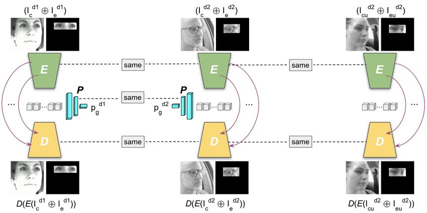
Figure 4: Our multi-domain training pipeline: For every iteration, the model is trained with mini-batches consisting of labeled input samples from d1
((Id1    d1               d2    d2                                        d2     d2
   c ⊕ Ie )) and d2 ((Ic ⊕ Ie )), and unlabeled input from d2 ((Icu ⊕ Ieu )). The model weights are updated based on the overall loss accumulated over
the mini-batches. It is to be noted that all three subjects in this figure are looking at the road, but appear very different due to different camera angles.

where N is training batch and C the ground truth classes.                            Our multi-domain training starts with three input tensors:
   The reconstruction loss Lprec is calculated for both the                       (1) (Id1    d1
                                                                                        c ⊕ Ie ) - the labeled face crop and eye patch images
current frame and baseline tensors as:                                            from the richly labeled domain d1,
                                                                                  (2) (Id2    d2
                                                                                        c ⊕ Ie ) - the labeled face crop and eye patch images
                    N                                                             from the sparsely labeled second domain d2,
              1 X
   Lprec =          |(Ic ⊕ Ie ) − D(E(Ic ⊕ Ie ))| +                               (3) (Id2    d2
                                                                                        cu ⊕ Ieu ) - the unlabeled face crop and eye patch im-
             |N | 1
                                                                                  ages from the second domain d2.
                        N
                  1 X
                        |(Bc ⊕ Be ) − D(E(Bc ⊕ Be ))| (5)                             Each tensor is passed through the encoder E to generate
                 |N | 1
                                                                                  their embedding, which are then passed through D to re-
The overall objective Lp is a weighted sum of these two                           construct the input. For the input tensors with glance labels
losses, calculated as:                                                            (i.e. (Id1   d1        d2    d2
                                                                                          c ⊕ Ie ) and (Ic ⊕ Ie )), the encoded feature is also
                                                                                  passed through the prediction head P to get the glance pre-
                        Lp = Lpcls + λ2 Lprec                          (6)        dictions pd1       d2
                                                                                             g and pg respectively. We set shareable weights
                                                                                  across the multi-streams of E, D and P during training, as
4.3. Domain Invariance                                                            shown in Figure 4.
    As can be seen in Figure 2, driver glance can look sig-
nificantly different when the camera type (RGB or NIR), its                           The classification loss Lmd
                                                                                                               cls for the multi-domain training
placement (steering wheel or rear-view mirror) and car in-                        is set as:
terior changes. Such a domain mismatch can result in con-
siderable decrease in performance when the classification
model is trained on one dataset and tested on another, as ex-                                      N  C       d1
                                                                                                 1 X X d1
perimentally shown in Section 5. To mitigate this domain                             Lmd
                                                                                      cls   = − d1      (c )i log(P (E(Id1   d1
                                                                                                                        c ⊕ Ie ))i )−
inconsistency problem, we propose a multi-domain training                                      |N | 1 i g
regime for our two-channel hourglass model. This regime                                              N  Cd2
                                                                                                1 X X d2
leverages a rich set of labeled training images from one do-                                              (c )i log(P (E(Id2   d2
                                                                                                                          c ⊕ Ie ))i ) (7)
main (e.g. MIT2013 dataset) to learn domain invariant fea-                                    |N d2 | 1 i g
tures for glance estimation from training samples from a
second domain (e.g. AVT or In-house dataset), only some
of which are labeled. The hourglass structure of our model
provides an advantage as the unlabeled samples from the                           where N d1 and N d2 are the labeled training batches, and
second domain can also be utilized during training using                          cd1     d2
                                                                                   g and cg are the ground truth glance labels from domains
D’s reconstruction error.                                                         d1 and d2 respectively.

                                                                             5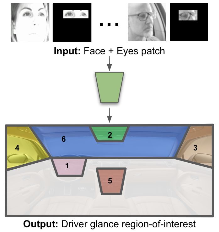
Table 1: Class-wise performance (ROC-AUC) of the different glance classification models on the MIT2013 dataset.

                                                                     Instrument                   Rearview                         Macro
                             Model                   Centerstack                       Left                    Right   Road
                                                                       Cluster                     Mirror                         Average
              Landmarks + MLP [16]                       0.907          0.892         0.960        0.919       0.886   0.835       0.900
                Baseline CNN [33]                        0.977          0.939         0.970        0.978       0.911   0.948       0.954
              One-Channel Hourglass                      0.979          0.945         0.976        0.983       0.927   0.946       0.960
         Two-Channel Hourglass (proposed)                0.983          0.956         0.978        0.980       0.930   0.961       0.965
         Personalized Hourglass (proposed)               0.983          0.953         0.981        0.982       0.941   0.959       0.967

     Table 2: Multi-domain performance (ROC-AUC) of our hourglass model, trained using different regimes, on the MIT2013 and AVT datasets.

                                                  Instrument                        Rearview                                            Macro
         Model                  Centerstack                         Left                               Right           Road
                                                    Cluster                          Mirror                                            Average
    Mixed Training              0.977, 0.969      0.956, 0.731   0.976, 0.961      0.980, 0.951     0.924, 0.977   0.944, 0.949      0.959, 0.923
    Fine-tuning[7]              0.891, 0.970      0.689, 0.732   0.938,0.963       0.930, 0.942     0.868, 0.953   0.880, 0.950      0.866, 0.918
 Gradient Reversal[18]          0.977, 0.964      0.946, 0.734   0.974, 0.945      0.979, 0.950     0.930, 0.976   0.944, 0.938      0.958, 0.918
         Ours                   0.974, 0.966      0.953, 0.793   0.972, 0.966      0.976, 0.955     0.934, 0.970   0.945, 0.935      0.959, 0.930

   Similarly, the reconstruction error Lmd
                                        rec is calculated as:                   generate the facial image and the eye patch was cropped out
                                                                                (also 96×96×1 in size) using the eye-landmarks extracted
                         d1
                  N
             1 X d1                                                             using the FAN network from [25], as can be seen in Figure
  Lmd
   rec   =           (Ic ⊕ Id1         d1   d1
                            e ) − D(E(Ic ⊕ Ie )) +                              1. Any frame with no detected faces was removed.
           |N d1 | 1
                   d2
                                                                                   During training, we use the Adam optimizer [30] with
              N
         1 X d2                                                                 the base learning rate set as 10−4 with a Dropout [61] layer
                 (Ic ⊕ Id2         d2   d2
                        e ) − D(E(Ic ⊕ Ie )) +
       |N d2 | 1                                                                (rate=0.7) between the dense layers of the prediction head
                        d2
                                                                                in the two-channel hourglass network (Section 4.1). The
                    Nu
               1 X                                                              weighing scalars λ1 , λ2 and λ3 are empirically set as 1 1
                       (Id2    d2          d2    d2
                         cu ⊕ Ieu ) − D(E(Icu ⊕ Ieu ))             (8)          and 10 respectively. We train all models using Tensorflow
             |Nud2 | 1
                                                                                [1] coupled with Keras [9] on a single NVIDIA Tesla V100
where Nud2 is the unlabeled training batch from domain d2.                      card with the batch size set as 8. For the personalized model
  The full multi-domain loss Lmd is calculated as:                              however, we find it optimal to train with a batch size of
                                                                                16 and learning rate of 10−3 . To reduce computation cost
                        Lmd = Lmd        md
                               cls + λ3 Lrec                       (9)          and further prevent overfitting, we stop model training once
                                                                                the validation loss plateaus across three epochs and save the
The weighing scalars λ1 (3), λ3 (6) and λ3 (9) are hyper-                       model snapshot for testing. We only use the trained encoder
parameters that are tuned experimentally.                                       and prediction head during inference.

5. Experiments                                                                     For training the personalization framework, we prepare
                                                                                multiple mini-batches for every iteration with the current
5.1. Training Details                                                           frame (Ic , Ie ) and baseline frame (Bc , Be ) inputs. For the
    To train our models we use ∼235K video frames from                          domain invariant regimen, the mini-batches are prepared
the MIT2013 dataset, and ∼153K and ∼163K for valida-                            with labeled d1 ((Id1    d1                 d2    d2
                                                                                                    c ⊕Ie )), labeled d2 ((Ic ⊕Ie )) and un-
                                                                                                      d2    d2
tion and testing respectively. The videos were split of-                        labeled d2 inputs ((Icu ⊕Ieu )). The overall loss is computed
fline to assign into training, validation and testing buckets.                  from the mini-batches before updating model weights.
Due to the large amount of labeled samples, we also use
                                                                                    Computation Overhead: In terms of model size, the
this dataset to represent the richly labeled domain (i.e. d1)
                                                                                encoder E and prediction head P together consist of 24M
for our domain invariant experiments, while using the AVT
                                                                                parameters while adding the decoder D for reconstruction
or In-house datasets as the second domain d2 (check Sec-
                                                                                increases the number to 54M. While D does add compu-
tion 4.3). We randomly sample ∼204K frames (Training:
                                                                                tational load during training, only E and P together are re-
162K, Validation: 22K, Testing: 20K) from the AVT and
                                                                                quired for inference. Thus, turning the typical classifier into
∼377K video frames (Training: 240K, Validation: 65K,
                                                                                an hourglass does not introduce additional overhead when
Testing: 72K) from the In-house datasets for these exper-
                                                                                deployed in production. The personalized version of the
iments3 . All frames were downsampled to 96×96×1 to
                                                                                model has the same number of trainable parameters but does
   3 Check   Section 9 for classwise breakdown.                                 require an additional stream of baseline driver information.

                                                                           6
Table 3: Multi-domain performance (ROC-AUC) of our hourglass model, trained using different regimes, on the MIT2013 and the In-house dataset.
Instrument Rearview Macro
Model Centerstack Left Right Road
Cluster Mirror Average
Mixed Training 0.977, 0.893 0.952, 0.779 0.978, 0.930 0.980, 0.933 0.933, 0.946 0.949, 0.838 0.962, 0.887
Fine-tuning[7] 0.706, 0.912 0.737, 0.799 0.877, 0.909 0.784, 0.915 0.727, 0.938 0.718, 0.835 0.758, 0.885
Gradient Reversal[18] 0.975, 0.888 0.931, 0.774 0.967, 0.894 0.978, 0.922 0.918, 0.929 0.932, 0.803 0.950, 0.868
Ours 0.975, 0.903 0.944, 0.810 0.974, 0.920 0.976, 0.926 0.925, 0.925 0.947, 0.835 0.957, 0.887
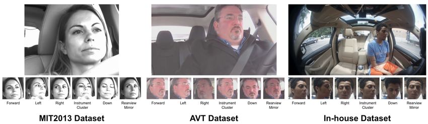
Figure 5: tSNE [66] visualization of the encoded features: Our multi-domain training more compactly packs together the feature samples from d1 (MIT2013)
and d2 (In-house dataset) than mixed-training, especially for the critical ‘Road’ class (in black).
5.2. Performance on the MIT2013 Dataset mation while requiring no extra stream of data.
Post training, we test our two-channel hourglass and per-
5.3. Domain Invariance
sonalization models for glance estimation on the test frames
For the domain invariance task, as described in Section
from the MIT2013 dataset[41]. To gauge of their effective-
4.3, we assign the MIT2013 dataset as the richly labeled
ness, we compare our model with the following:
domain d1 as it has a large number of video frames with
(1) Landmarks + MLP. Following [16], we train a baseline
human-annotated glance labels and use the AVT and our
MLP model with 3 dense layers on a flattened representa-
In-house datasets interchangeably as the new domain d2.
tion of facial landmarks extracted using [25].
To evaluate its effectiveness, we compare our multi-domain
(2) Baseline CNN. We also train a baseline CNN with 4
training approach with following regimes while keeping the
convolutional and max pooling layers followed by 3 dense
backbone network (two-channel hourglass) the same:
layers, similar to AlexNet [33]. The baseline CNN takes as
(1) Mixed Training. Only labeled data from d1 and d2 are
input the 96×96×1 cropped face image.
pooled together based on their glance labels for training.
(4) One-Channel Hourglass. This model only receives the
(2) Fine-tuning [7]. We train the model on labeled data
cropped face image Ic without the eye-patch channel Ie . The
from d1 and then fine-tune the saved snapshot on labeled
hyper-parameters and losses however remain the same.
data from d2, a strategy similar to [7].
As can be seen in Table 1, increasing the input quality (3) Gradient Reversal [18]. We add a domain classifica-
(e.g. landmarks vs. actual pixels) and model complexity tion block on top of the encoder output to predict the do-
(e.g. baseline CNN vs. residual encoder) also improves main of each input. However, its gradient is reversed during
classification performance, with both the personalization backpropagation to confuse the model and shift its repre-
multi-stream and hourglass models outperforming the other sentations towards a common manifold, similar to [18]4 .
approaches and the latter producing the best macro average Although our multi-domain training approach can utilize
ROC-AUC. This suggests providing the model with an ad- the unlabeled samples from d2, for our first experiment we
ditional stream of subject-specific information (i.e. person- use 100% of the annotated images from both d1 and d2 to
alization) can better tune the model with respect to move- level the playing field. The same model snapshot is used
ment of the driver head, as validated by the improved per- for testing on both the MIT2013 dataset (d1) and the AVT
formance on ’Instrument Cluster’, ’Left’ ’Right’ and ’Road’ or In-house datasets (d2). The results can be seen in Ta-
classes. Alternatively, adding an auxiliary reconstruction bles 2 and 3 respectively. In both cases, the fine-tuning ap-
task (i.e. adding decoder) can also boost the overall primary
classification accuracy by learning useful contextual infor- 4 We use the implementation from [62].
7Table 4: Performance (ROC-AUC) of our two-channel hourglass model with mixed training and our multi-domain regime, on the In-house dataset with
different amount of labeled samples. The utility of unlabeled samples paired with reconstruction loss is evident as the percentage of labeled data from the
second domain decreases.
Model (labeled data) Centerstack Instrument Cluster Left Rearview Mirror Right Road Macro Average
Mixed Training (50%) 0.876 0.785 0.920 0.936 0.922 0.828 0.877
Ours (50%) 0.897 0.818 0.944 0.943 0.938 0.842 0.897
Mixed Training (10%) 0.821 0.734 0.882 0.867 0.924 0.798 0.838
Ours (10%) 0.881 0.814 0.900 0.898 0.893 0.845 0.872
Mixed Training (1%) 0.776 0.704 0.859 0.775 0.854 0.696 0.777
Ours (1%) 0.830 0.790 0.904 0.847 0.852 0.777 0.833
Table 5: Performance (ROC-AUC) of our two-channel hourglass model with different components ablated on the MIT2013 dataset.
Model Centerstack Instrument Cluster Left Rearview Mirror Right Road Macro Average
w/ MSE 0.977 0.944 0.975 0.974 0.934 0.941 0.957
wo/ skip connections 0.980 0.942 0.974 0.981 0.935 0.943 0.959
wo/ Lrec 0.977 0.945 0.976 0.978 0.926 0.946 0.958
wo/ Lcls [7] 0.979 0.936 0.974 0.976 0.933 0.952 0.958
Full Model 0.983 0.956 0.978 0.980 0.930 0.961 0.965
proach fails to generalize to both domains, essentially “for- tions of our model:
getting” details of the initial task (i.e. d1). Adding the gra- (1) w/ MSE. Instead of mean absolute error, the reconstruc-
dient reversal head, does generate a boost over fine-tuning, tion loss is computed with mean squared error.
however it overfits slightly on the training set and takes al- (2) wo/ skip connections. We remove skip connections be-
most twice as the other approaches to converge. The mixed tween the encoder and decoder layers.
training and our multi-domain approaches perform compet- (3) wo/ Lrec . The reconstruction loss is removed, essen-
itively and generate the best ROC-AUC numbers on the tially making the model a traditional classification module
MIT2013-Inhouse and MIT2013-AVT respectively. with residual layers.
However, using all labeled data from the new domain (4) wo/ Lcls . Taking inspiration from [7], we first train the
does not fairly evaluate the full potential of our approach. hourglass solely with the reconstruction task (i.e. no Lcls )
Unlike the other approaches, our training regimen can uti- and then use the encoder module as a feature extractor to
lize the unlabeled data (i.e. (Id2 d2
cu ⊕ Ieu )) via the reconstruc-
train the prediction block. For all the model variations, we
tion loss, as proposed in Section 4.3. To put this functional- keep everything else the same for consistency.
ity into effect, we use different amount of labeled samples As presented in Table 5, ablating the different com-
(50%, 10% and 1%) from d2 during training the hourglass ponents generates slightly different results. Due to the
model with mixed training and multi-domain regimes. As pixel normalization between [−1, 1] before training, using
shown in Table 4, our approach significantly outperforms MSE based reconstruction slightly dampens the error due to
mixed training as the amount of labeled data in the new squaring. The skip connections help in propagating stronger
domain diminishes. Interestingly, our multi-domain hour- signals across the network [51], hence removing them neg-
glass trained with 50% labeled data generalizes better than atively affects model performance. Removing Lrec alto-
when trained with 100% labeled data suggesting more gen- gether deteriorates model performance as contextual infor-
eralizable global features are learned when an unsupervised mation gets overlooked. Surprisingly, unsupervised pre-
component is added to a classification task. This is further training performs quite well, suggesting the reconstruction
validated when visualizing the encoded features using tSNE task can teach the model features useful for classification.
[66], as depicted in Figure 5. Our multi-domain training This reconstruction element, present in our full model, helps
more compactly packs together the feature samples from it achieve the best overall performance.
d1 and d2 than mixed-training, especially for the critical
‘Road’ class. Thus, this technique can be used to gauge the 6. Conclusion
amount of labeling required when adapting models to new Advanced driver assistance systems that can detect
domains and consequently reduce annotation cost. whether a driver is distracted can help improve driver safety
but pose many research challenges. In this work, we pro-
5.4. Ablation Studies posed a model that takes as input a patch of the driver’s face
To check the contribution of each component of our two- along with a crop of the eye-region and provides a clas-
channel hourglass network, we train the following varia- sification into 6 coarse ROIs in the vehicle. We demon-
8strated that an hourglass network consisting of encoder- IEEE International Conference on Computer Vision Work-
decoder modules, trained with a secondary reconstruction shops, pages 0–0, 2019. 2
loss, allows the model to learn strong feature representa- [7] M. Chen, A. Radford, R. Child, J. Wu, H. Jun, D. Luan, and
tions and perform better in the primary glance classification I. Sutskever. Generative pretraining from pixels. In Interna-
task. In order to make the system more robust to subject- tional Conference on Machine Learning (ICML), 2020. 6, 7,
8
specific variations in appearance and driving behavior, we
[8] Rishu Chhabra, Seema Verma, and C Rama Krishna. A sur-
proposed a multi-stream model that takes a representation
vey on driver behavior detection techniques for intelligent
of a driver’s baseline glance behavior as an auxiliary input transportation systems. In 2017 7th International Confer-
for learning residuals. Results indicate such personalized ence on Cloud Computing, Data Science & Engineering-
training to improve model performance for multiple glance Confluence, pages 36–41. IEEE, 2017. 2
ROIs over rigid models. [9] F. Chollet et al. Keras. https : / / github . com /
Finally, we designed a multi-domain training regime to fchollet/keras, 2015. 6
jointly train our hourglass model on data collected from [10] Wen-Sheng Chu, Fernando De la Torre, and Jeffery F Cohn.
multiple camera views. Leveraging the hourglass’ auxil- Selective transfer machine for personalized facial action unit
iary reconstruction objective, this approach can learn do- detection. In Proceedings of the IEEE Conference on Com-
main invariant representations from very little labeled data puter Vision and Pattern Recognition, pages 3515–3522,
2013. 2
in a weakly supervised manner, and consequently reduce la-
[11] Joseph F Coughlin, Bryan Reimer, and Bruce Mehler. Mon-
beling cost. As a future work, we plan to use our hourglass
itoring, managing, and motivating driver safety and well-
model as a proxy for annotating unlabeled data from new being. IEEE Pervasive Computing, 10(3):14–21, 2011. 1
domains and actively learn from high confidence samples. [12] J. Deng, J. Guo, N. Xue, and S. Zafeiriou. Arcface: Ad-
ditive angular margin loss for deep face recognition. In
7. Acknowledgements IEEE Conference on Computer Vision and Pattern Recog-
nition (CVPR), 2019. 2
The AVT and MIT 2013 dataset used in this study were [13] X. Dong, S. Yu, X. Weng, S. Wei, Y. Yang, and Y. Sheikh.
drawn from work supported by the Advanced Vehicle Tech- Supervision-by-registration: An unsupervised approach to
nologies (AVT) Consortium at MIT (http://agelab. improve the precision of facial landmark detectors. In IEEE
mit.edu/avt) and the Insurance Institute for Highway Conference on Computer Vision and Pattern Recognition
Safety (IIHS) respectively. (CVPR), 2018. 3
[14] Gregory M Fitch, Susan A Soccolich, Feng Guo, Julie Mc-
Clafferty, Youjia Fang, Rebecca L Olson, Miguel A Perez,
References Richard J Hanowski, Jonathan M Hankey, and Thomas A
[1] M. Abadi, P. Barham, J. Chen, Z. Chen, A. Davis, J. Dean, Dingus. The impact of hand-held and hands-free cell phone
M. Devin, S. Ghemawat, G. Irving, M. Isard, M. Kudlur, J. use on driving performance and safety-critical event risk.
Levenberg, R. Monga, S. Moore, D.G. Murray, B. Steiner, Technical report, 2013. 1
P. Tucker, V. Vasudevan, P. Warden, M. Wicke, Y. Yu, and [15] Lex Fridman, Daniel E Brown, Michael Glazer, William An-
X. Zheng. Tensorflow: A system for large-scale machine gell, Spencer Dodd, Benedikt Jenik, Jack Terwilliger, Alek-
learning. In 12th USENIX Conference on Operating Systems sandr Patsekin, Julia Kindelsberger, Li Ding, et al. Mit ad-
Design and Implementation, pages 265–283, 2016. 6 vanced vehicle technology study: Large-scale naturalistic
driving study of driver behavior and interaction with automa-
[2] S. Banerjee, W. Scheirer, K. Bowyer, and P. Flynn. Fast face
tion. IEEE Access, 7:102021–102038, 2019. 3, 12, 13
image synthesis with minimal training. In IEEE Winter Con-
ference on Applications of Computer Vision, 2019. 2 [16] Lex Fridman, Joonbum Lee, Bryan Reimer, and Trent Vic-
tor. ‘owl’and ‘lizard’: Patterns of head pose and eye pose in
[3] S. Banerjee, W. Scheirer, K. Bowyer, and P. Flynn. On hal-
driver gaze classification. IET Computer Vision, 10(4):308–
lucinating context and background pixels from a face mask
314, 2016. 2, 3, 6, 7
using multi-scale gans. In IEEE Winter Conference on Ap-
[17] Lex Fridman, Bryan Reimer, Bruce Mehler, and William T
plications of Computer Vision (WACV), 2020. 4
Freeman. Cognitive load estimation in the wild. In Proceed-
[4] D. Blalock, J. J. Gonzalez Ortiz, J. Frankle, and J. Guttag. ings of the 2018 chi conference on human factors in comput-
What is the state of neural network pruning? In Machine ing systems, pages 1–9, 2018. 2
Learning and Systems (MLSys), 2020. 2 [18] Y. Ganin, E. Ustinova, H. Ajakan, P. Germain, H. Larochelle,
[5] Dario Cazzato, Marco Leo, Cosimo Distante, and Holger F. Laviolette, M. March, and V. Lempitsky. Domain-
Voos. When i look into your eyes: A survey on computer adversarial training of neural networks. Journal of Machine
vision contributions for human gaze estimation and tracking. Learning Research (JMLR), 17(59):1–35, 2016. 2, 6, 7
Sensors, 20(13):3739, 2020. 2 [19] T. Gebru, J. Hoffman, and F-F. Li. Fine-grained recognition
[6] Zhuoqing Chang, J Matias Di Martino, Qiang Qiu, Steven in the wild: A multi-task domain adaptation approach. In
Espinosa, and Guillermo Sapiro. Salgaze: Personalizing IEEE International Conference on Computer Vision (ICCV),
gaze estimation using visual saliency. In Proceedings of the 2017. 2
9[20] Shreya Ghosh, Abhinav Dhall, Garima Sharma, Sarthak crash risk from glance patterns in naturalistic driving. Hu-
Gupta, and Nicu Sebe. Speak2label: Using domain knowl- man Factors, 54(6):1104–1116, 2012. 1
edge for creating a large scale driver gaze zone estimation [35] Erik Lindén, Jonas Sjostrand, and Alexandre Proutiere.
dataset. arXiv preprint arXiv:2004.05973, 2020. 2 Learning to personalize in appearance-based gaze tracking.
[21] Dan Witzner Hansen and Qiang Ji. In the eye of the beholder: In Proceedings of the IEEE International Conference on
A survey of models for eyes and gaze. IEEE transactions on Computer Vision Workshops, pages 0–0, 2019. 2
pattern analysis and machine intelligence, 32(3):478–500, [36] W. Liu, Y. Wen, Z. Yu, M. Li, B. Raj, and S. Le. Sphereface:
2009. 2 Deep hypersphere embedding for face recognition. In IEEE
[22] M. Haris, G. Shakhnarovich, and N. Ukita. Task-driven super Conference on Computer Vision and Pattern Recognition
resolution: Object detection in low-resolution images. arXiv (CVPR), 2017. 2
preprint arXiv:1803.11316, 2018. 3
[37] Alireza Makhzani, Jonathon Shlens, Navdeep Jaitly, and Ian
[23] K. He, X. Zhang, S. Ren, and J. Sun. Deep residual learning
Goodfellow. Adversarial autoencoders. In International
for image recognition. In IEEE Conference on Computer
Conference on Learning Representations (ICLR), 2016. 3
Vision and Pattern Recognition (CVPR), 2016. 3, 4, 12
[38] A. Mallya, D. Davis, and S. Lazebnik. Piggyback: Adapt-
[24] M. Huh, P. Agarwal, and AA. Efros. What makes
ing a single network to multiple tasks by learning to mask
imagenet good for transfer learning? arXiv preprint
weights. In European Conference on Computer Vision
arXiv:1608.08614, 2016. 2
(ECCV), 2018. 2
[25] A. S. Jackson, A. Bulat, V. Argyriou, and G. Tzimiropoulos.
Large pose 3d face reconstruction from a single image via [39] A. Mallya and S. Lazebnik. Packnet: Adding multiple tasks
direct volumetric cnn regression. IEEE International Con- to a single network by iterative pruning. In IEEE Conference
ference on Computer Vision (ICCV), 2017. 6, 7 on Computer Vision and Pattern Recognition (CVPR), 2018.
[26] Sumit Jha and Carlos Busso. Probabilistic estimation of the 2
gaze region of the driver using dense classification. In 2018 [40] I. Masi, A. T. Tran, J. T. Leksut, T. Hassner, and G. Medioni.
21st International Conference on Intelligent Transportation Do we really need to collect millions of faces for effective
Systems (ITSC), pages 697–702. IEEE, 2018. 2 face recognition? In European Conference on Computer
[27] Ajjen Joshi, Soumya Ghosh, Margrit Betke, Stan Sclaroff, Vision, 2016. 2
and Hanspeter Pfister. Personalizing gesture recognition us- [41] Bruce Mehler, David Kidd, Bryan Reimer, Ian Reagan,
ing hierarchical bayesian neural networks. In Proceedings Jonathan Dobres, and Anne McCartt. Multi-modal assess-
of the IEEE Conference on Computer Vision and Pattern ment of on-road demand of voice and manual phone calling
Recognition, pages 6513–6522, 2017. 2 and voice navigation entry across two embedded vehicle sys-
[28] Ajjen Joshi, Survi Kyal, Sandipan Banerjee, and Taniya tems. Ergonomics, 59(3):344–367, 2016. 3, 7, 12, 13, 14
Mishra. In-the-wild drowsiness detection from facial expres- [42] Alberto Morando, Pnina Gershon, Bruce Mehler, and Bryan
sions. In Proceedings of the IEEE Intelligent Vehicles Sym- Reimer. Driver-initiated tesla autopilot disengagements in
posium Human Sensing and Intelligent Mobility Workshop, naturalistic driving. In 12th International Conference on Au-
2020. 2 tomotive User Interfaces and Interactive Vehicular Applica-
[29] Joohwan Kim, Michael Stengel, Alexander Majercik, Shalini tions, pages 57–65, 2020. 3
De Mello, David Dunn, Samuli Laine, Morgan McGuire, and [43] P. Morgado and N. Vasconcelos. Nettailor: Tuning the archi-
David Luebke. Nvgaze: An anatomically-informed dataset tecture, not just the weights. In IEEE Conference on Com-
for low-latency, near-eye gaze estimation. In Proceedings of puter Vision and Pattern Recognition (CVPR), 2019. 2
the 2019 CHI Conference on Human Factors in Computing
[44] M. Mostajabi, M. Maire, and G. Shakhnarovich. Regulariz-
Systems, pages 1–12, 2019. 2
ing deep networks by modeling and predicting label struc-
[30] D. Kingma and J. Ba. Adam: A method for stochastic op-
ture. In IEEE Conference on Computer Vision and Pattern
timization. In International Conference on Learning Repre-
Recognition (CVPR), 2018. 2, 3
sentations (ICLR), 2015. 6
[45] A. Newell, K. Yang, and J. Deng. Stacked hourglass net-
[31] S. Kornblith, J. Shlens, and QV. Le. Do better imagenet mod-
works for human pose estimation. In European Conference
els transfer better? In IEEE Conference on Computer Vision
on Computer Vision, 2016. 2
and Pattern Recognition (CVPR), 2019. 2
[32] Kyle Krafka, Aditya Khosla, Petr Kellnhofer, Harini Kan- [46] X. Peng, Z. Huang, X. Sun, and K. Saenko. Domain agnostic
nan, Suchendra Bhandarkar, Wojciech Matusik, and Anto- learning with disentangled representations. In International
nio Torralba. Eye tracking for everyone. In Proceedings of Conference on Machine Learning (ICML), 2019. 2
the IEEE conference on computer vision and pattern recog- [47] P.J. Phillips. A cross benchmark assessment of a deep convo-
nition, pages 2176–2184, 2016. 2 lutional neural network for face recognition. In IEEE Inter-
[33] A. Krizhevsky, I. Sutskever, and G. E. Hinton. Ima- national Conference on Automatic Face and Gesture Recog-
genet classification with deep convolutional neural networks. nition, 2017. 2
In Conference on Neural Information Processing Systems [48] A. Radford, L. Metz, and S. Chintala. Unsupervised rep-
(NeurIPS), 2012. 3, 6, 7, 14 resentation learning with deep convolutional generative ad-
[34] Yulan Liang, John D Lee, and Lora Yekhshatyan. How dan- versarial networks. In International Conference on Learning
gerous is looking away from the road? algorithms predict Representations (ICLR), 2016. 4, 12
10[49] Akshay Rangesh, Bowen Zhang, and Mohan M Trivedi. [62] M. Tonutti, E. Ruffaldi, A. Cattaneo, and CA. Avizzano. Ro-
Driver gaze estimation in the real world: Overcoming the bust and subject-independent driving manoeuvre anticipa-
eyeglass challenge. arXiv preprint arXiv:2002.02077, 2020. tion through domain-adversarial recurrent neural networks.
2 Robotics and Autonomous Systems, 115:162–173, 2019. 7
[50] A. Rice, P.J. Phillips, V. Natu, X. An, and A.J. O’Toole. Un- [63] E. Tzeng, J. Hoffman, T. Darrell, and K. Saenko. Simul-
aware person recognition from the body when face identi- taneous deep transfer across domains and tasks. In IEEE
fication fails. Psychological Science, 24:2235–2243, 2013. International Conference on Computer Vision (ICCV), 2015.
2 2
[51] O. Ronneberger, P. Fischer, and T. Brox. U-net: Convolu- [64] E. Tzeng, J. Hoffman, K. Saenko, and T. Darrell. Adversarial
tional networks for biomedical image segmentation. In In- discriminative domain adaptation. In IEEE Conference on
ternational Conference on Medical Image Computing and Computer Vision and Pattern Recognition (CVPR), 2017. 2
Computer Assisted Intervention (MICCAI), 2015. 2, 4, 8, [65] E. Tzeng, J. Hoffman, N. Zhang, K. Saenko, and T. Darrell.
12 Deep domain confusion: Maximizing for domain invariance.
[52] Olga Russakovsky, Jia Deng, Hao Su, Jonathan Krause, San- arXiv preprint arXiv:1412.3474, 2014. 2
jeev Satheesh, Sean Ma, Zhiheng Huang, Andrej Karpathy, [66] L.J.P. van der Maaten and G.E. Hinton. Visualizing high-
Aditya Khosla, Michael Bernstein, Alexander C. Berg, and dimensional data using t-sne. Journal of Machine Learning
Li Fei-Fei. ImageNet Large Scale Visual Recognition Chal- Research (JMLR), 9:2579–2605, 2008. 7, 8
lenge. International Journal of Computer Vision (IJCV), [67] Francisco Vicente, Zehua Huang, Xuehan Xiong, Fernando
115(3):211–252, 2015. 3 De la Torre, Wende Zhang, and Dan Levi. Driver gaze track-
[53] K. Saenko, B. Kulis, M. Fritz, , and T. Darrell. Adapting ing and eyes off the road detection system. IEEE Trans-
visual category models to new domains. In European Con- actions on Intelligent Transportation Systems, 16(4):2014–
ference on Computer Vision (ECCV), 2010. 2 2027, 2015. 2
[68] H. Wang, Y. Wang, Z. Zhou, X. Ji, D. Gong, J. Zhou, Z. Li,
[54] T. Salimans, I. Goodfellow, W. Zaremba, V. Cheung, A. Rad-
and W. Liu. Cosface: Large margin cosine loss for deep face
ford, and X. Chen. Improved techniques for training gans.
recognition. In IEEE Conference on Computer Vision and
In Conference on Neural Information Processing Systems
Pattern Recognition (CVPR), 2018. 2
(NeurIPS), 2016. 4, 12
[69] Y. Wen, K. Zhang, Z. Li, and Y. Qiao. A discriminative fea-
[55] Bobbie D Seppelt, Sean Seaman, Joonbum Lee, Linda S An-
ture learning approach for deep face recognition. In Euro-
gell, Bruce Mehler, and Bryan Reimer. Glass half-full: On-
pean Conference on Computer Vision (ECCV), 2016. 2
road glance metrics differentiate crashes from near-crashes
[70] Erroll Wood, Tadas Baltrušaitis, Louis-Philippe Morency,
in the 100-car data. Accident Analysis & Prevention, 107:48–
Peter Robinson, and Andreas Bulling. Learning an
62, 2017. 1
appearance-based gaze estimator from one million synthe-
[56] V. Sharma, A. Diba, D. Neven, MS. Brown, L. Van Gool,
sised images. In Proceedings of the Ninth Biennial ACM
and R. Stiefelhagen. Classification-driven dynamic image
Symposium on Eye Tracking Research & Applications, pages
enhancement. In IEEE Conference on Computer Vision and
131–138, 2016. 2
Pattern Recognition (CVPR), 2018. 3
[71] Erroll Wood, Tadas Baltrusaitis, Xucong Zhang, Yusuke
[57] W. Shi, J. Caballero, F. Huszar, J. Totz, A.P. Aitken, R. Sugano, Peter Robinson, and Andreas Bulling. Rendering of
Bishop, D. Rueckert, and Z. Wang. Real-time single image eyes for eye-shape registration and gaze estimation. In Pro-
and video super-resolution using an efficient sub-pixel con- ceedings of the IEEE International Conference on Computer
volutional neural network. In IEEE Conference on Computer Vision, pages 3756–3764, 2015. 2
Vision and Pattern Recognition (CVPR), 2016. 4, 12 [72] Angela Yao, Luc Van Gool, and Pushmeet Kohli. Gesture
[58] Ashish Shrivastava, Tomas Pfister, Oncel Tuzel, Joshua recognition portfolios for personalization. In Proceedings
Susskind, Wenda Wang, and Russell Webb. Learning of the IEEE Conference on Computer Vision and Pattern
from simulated and unsupervised images through adversarial Recognition, pages 1915–1922, 2014. 2
training. In Proceedings of the IEEE conference on computer [73] F. Yu and V. Koltun. Multi-scale context aggregation by di-
vision and pattern recognition, pages 2107–2116, 2017. 2 lated convolutions. In International Conference on Learning
[59] K. Simonyan and A. Zisserman. Very deep convolutional Representations (ICLR), 2016. 4, 12
networks for large-scale image recognition. In International [74] Yu Yu, Gang Liu, and Jean-Marc Odobez. Improving few-
Conference on Learning Representations (ICLR), 2015. 3 shot user-specific gaze adaptation via gaze redirection syn-
[60] David L Smith, James Chang, Richard Glassco, James Foley, thesis. In Proceedings of the IEEE Conference on Computer
and Daniel Cohen. Methodology for capturing driver eye Vision and Pattern Recognition, pages 11937–11946, 2019.
glance behavior during in-vehicle secondary tasks. Trans- 2
portation research record, 1937(1):61–65, 2005. 3 [75] Xucong Zhang, Yusuke Sugano, Mario Fritz, and Andreas
[61] Nitish Srivastava, Geoffrey Hinton, Alex Krizhevsky, Ilya Bulling. Mpiigaze: Real-world dataset and deep appearance-
Sutskever, and Ruslan Salakhutdinov. Dropout: A simple based gaze estimation. IEEE transactions on pattern analy-
way to prevent neural networks from overfitting. Journal sis and machine intelligence, 41(1):162–175, 2017. 2
of Machine Learning Research (JMLR), 15(56):1929–1958, [76] Y. Zheng, DK. Pal, and M. Savvides. Ring loss: Convex fea-
2014. 6, 12 ture normalization for face recognition. In IEEE Conference
11Table 6: Encoder E architecture (input size is 96×96×2) Table 7: Decoder D architecture (input size is (512,)
Layer Filter/Stride/Dilation # of filters Layer Filter/Stride/Dilation # of filters
conv1 3×3/1/2 128 fc2 3*3*1024 -
conv2 3×3/2/1 64 conv7 3×3/1/1 4*512
RB1 3×3/1/1 64 PS1 - -
conv3 3×3/2/1 128 conv8 3×3/1/1 4*256
RB2 3×3/1/1 128 PS2 - -
conv4 3×3/2/1 256 conv9 3×3/1/1 4*128
RB3 3×3/1/1 256 PS3 - -
conv5 3×3/2/1 512 conv10 3×3/1/1 4*64
RB4 3×3/1/1 512 PS4 - -
conv6 3×3/2/1 1,024 conv11 3×3/1/1 4*64
RB5 3×3/1/1 1,024 PS5 - -
fc1 512 - conv12 5×5/1/1 2
Table 8: Prediction head P architecture (input size is (512,)
on Computer Vision and Pattern Recognition (CVPR), 2018. Layer Filter/Stride/Dilation # of filters
2
fc3 256 -
fc4 6 -
9. Classwise Data Distribution
Here we present the class wise distribution of samples
for the MIT2013 [41], AVT [15] and our In-house collected
8. Detailed Model Architecture datasets in Figure 6. As can be seen, the pre-dominant class
(ROI) is the driver actually looking on the road (‘Road’),
Here we describe in detail the architecture of the en- especially for the MIT2013 and In-house datasets. This
coder E and decoder D modules, and the prediction head imbalance can cause the trained model’s representations to
P of our two-channel hourglass model. As discussed in be skewed towards the largely populated ROIs and perform
Section 4.1 of the main text, E takes as input a 96×96×2 poorly for the sparse classes. However, as presented in the
input and passes it through a dilated convolution layer [73] results from the main text our model does not exhibit such
before followed by 5 residual blocks [23] with stride = 2 bias and performs competitively for all the ROI classes.
for downsampling. This downsampled output is fed to a
densely connected layer with 512 neurons and linear acti- 10. Reconstruction Example
vation to generate the encoded feature representation of the
input. D is designed like a mirror image of E and takes We present a random set of face samples from our In-
this dense 512-D input and feeds it through 5 upsampling house dataset and their reconstructions generated by our
pixel shuffling layers [57]. We also add skip connections hourglass model in Figure 7. Except for some noise and
[51] between layers in E and D with the same feature map grid-like artifact in some cases, we find there to be little dif-
resolution for stronger signal propagation. The final upsam- ference between the input and reconstructed images.
pled output is passed through a convolution layer with tanh
activation to reconstruct the 96×96×2 input [48, 54]. P 11. Confusion Matrices
is composed of two dense layers with a dropout [61] layer In the main text, we utilize ROC-AUC as the metric
in between for regularization. We apply softmax activation to report performance of the different models. Since the
for the second dense layer to get the final glance prediction. ROC-AUC metric is threshold agnostic, it can be used to
Unless stated otherwise, all layers use a leaky ReLU activa- gauge model performance while sweeping through differ-
tion. ent thresholds. However, we also present the performance
The detailed layers of E, D and P are listed in Tables 6, of each of our candidate models on the MIT2013 [41] test
7, and 8 respectively. The convolution layers, dense layers, set in Figure 8 using confusion matrices normalized by total
residual blocks and pixel shuffling blocks are represented as samples for each class.
‘conv’, ‘fc’, ‘RB’, and ‘PS’ respectively in the tables.
12Figure 6: Class wise distribution of samples in the Train, Validation and Test splits in the MIT2013 [41], AVT [15] and our In-house datasets. The
‘Centerstack’, ‘Instrument Cluster’ and ‘Rearview Mirror’ are abbreviated as ‘CS’, ‘IC’ and ‘RVM’.
Figure 7: Randomly sampled cropped face images (input) and their reconstructions produced by our hourglass model. Subtle differences between the two
sets can be observed by zooming in. All images are 96×96×1 in resolution.
13Figure 8: Normalized confusion matrices across the different classes on the MIT2013 [41] test samples using - (a) Landmarks + MLP model, (b) Baseline
CNN [33], (c) One-Channel Hourglass, (d) Two-Channel Hourglass, and (e) Personalized Hourglass model.
14You can also read