Semi-supervised adversarial neural networks classification
←
→
Page content transcription
If your browser does not render page correctly, please read the page content below
Downloaded from genome.cshlp.org on April 17, 2021 - Published by Cold Spring Harbor Laboratory Press

Semi-supervised              adversarial             neural          networks             for       single-cell
classification

                   Jacob C. Kimmel                                        David R. Kelley
               Calico Life Sciences, LLC                             Calico Life Sciences, LLC
           South San Francisco, CA, 94080                         South San Francisco, CA, 94080
               jacob@calicolabs.com                                    drk@calicolabs.com
                                                                           * Lead Contact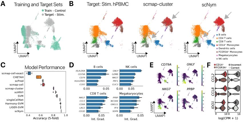
Downloaded from genome.cshlp.org on April 17, 2021 - Published by Cold Spring Harbor Laboratory Press

                                                             Abstract

 1            Annotating cell identities is a common bottleneck in the analysis of single cell genomics experiments.
 2            Here, we present scNym, a semi-supervised, adversarial neural network that learns to transfer cell
 3            identity annotations from one experiment to another. scNym takes advantage of information in
 4            both labeled datasets and new, unlabeled datasets to learn rich representations of cell identity that
 5            enable effective annotation transfer. We show that scNym effectively transfers annotations across
 6            experiments despite biological and technical differences, achieving performance superior to existing
 7            methods. We also show that scNym models can synthesize information from multiple training and
 8            target datasets to improve performance. In addition to high accuracy, we show that scNym models
 9            are well-calibrated and interpretable with saliency methods.

10   Keywords single cell · neural network · cell type classification · semi-supervised learning · adversarial learning

11   Introduction

12   Single cell genomics allows for simultaneous molecular profiling of thousands of diverse cells and has advanced our
13   understanding of development [Trapnell, 2015], aging [Angelidis et al., 2019, Kimmel et al., 2019, Ma et al., 2020],
14   and disease [Tanay and Regev, 2017]. To derive biological insight from these data, each single cell molecular profile
15   must be annotated with a cell identity, such as a cell type or state label. Traditionally, this task has been performed
16   manually by domain expert biologists. Manual annotation is time consuming, somewhat subjective, and error prone.
17   Annotations influence the results of nearly all downstream analyses, motivating more robust algorithmic approaches for
18   cell type annotation.

19   Automated classification tools have been proposed to transfer annotations across datasets [Kiselev et al., 2018,
20   Alquicira-Hernandez et al., 2019,           Tan and Cahan, 2019,       Abdelaal et al., 2019,       de Kanter et al., 2019,
21   Pliner et al., 2019, Zhang et al., 2019].      These existing tools learn relationships between cell identity and
22   molecular features from a training set with existing labels without considering the unlabeled target dataset in
23   the learning process. However, results from the field of semi-supervised representation learning suggest that
24   incorporating information from the target data during training can improve the performance of prediction models
25   [Kingma et al., 2014, Oliver et al., 2018, Verma et al., 2019, Berthelot et al., 2019].     This approach is especially
26   beneficial when there are systematic differences – a domain shift – between the training and target datasets. Domain
27   shifts are commonly introduced between single cell genomics experiments when cells are profiled in different
28   experimental conditions or using different sequencing technologies.

29   A growing family of representation learning techniques encourage classification models to provide consistent
30   interpolations between data points as an auxiliary training task to improve performance [Verma et al., 2019,
31   Berthelot et al., 2019]. In the semi-supervised setting, the MixMatch approach implements this idea by “mixing”

                                                                 2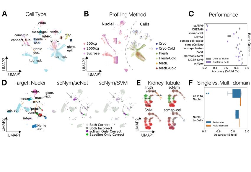
Downloaded from genome.cshlp.org on April 17, 2021 - Published by Cold Spring Harbor Laboratory Press

32   observations and their labels with simple weighted averages. Mixed observations from the training and target datasets
33   form a bridge in feature space, encouraging the model to learn a smooth interpolation across the domains. Another
34   family of techniques seek to improve classification performance in the presence of domain shifts by encouraging
35   the model to learn a representation in which observations from different domains are embedded nearby, rather than
36   occupying distinct regions of a latent space [Wilson and Cook, 2020]. One successful approach uses a “domain ad-
37   versary” to encourage the classification model to learn a representation that is invariant to dataset-specific features
38   [Ganin et al., 2016]. Both interpolation consistency and domain invariance are desirable in the single cell genomics
39   setting, where domain shifts are common and complex gene expression boundaries separate cell types.

40   Here, we introduce a cell type classification model that uses semi-supervised and adversarial machine learning
41   techniques to take advantage of both labeled and unlabeled single cell datasets. We demonstrate that this model offers
42   superior performance to existing methods and effectively transfers annotations across different animal ages, perturbation
43   conditions, and sequencing technologies. Additionally, we show that our model learns biologically interpretable
44   representations and offers well-calibrated metrics of annotation confidence that can be used to make new cell type
45   discoveries.

46   Results

47   scNym

48   In the typical supervised learning framework, the model touches the target unlabeled dataset to predict labels only
49   after training has concluded. By contrast, our semi-supervised learning framework trains the model parameters on
50   both the labeled and unlabeled data in order to leverage the structure in the target dataset, whose measurements may
51   have been influenced by myriad sources of biological and technical bias and batch effects. While our model uses
52   observed cell profiles from the unlabeled target dataset, at no point does the model access ground truth labels for the
53   target data. Ground truth labels on the target dataset are used exclusively to evaluate model performance. Some single
54   cell classification methods require manual marker gene specification prior to model training. scNym requires no prior
55   manual specification of marker genes, but rather learns relevant gene expression features from the data.

56   scNym uses the unlabeled target data through a combination of MixMatch semi-supervision [Berthelot et al., 2019] and
57   by training a domain adversary [Ganin et al., 2016] in an iterative learning process (Fig. 1A, Methods). The MixMatch
58   semi-supervision approach combines MixUp data augmentations [Zhang et al., 2018, Thulasidasan et al., 2019] with
59   pseudolabeling of the target data [Lee, 2013, Verma et al., 2019] to improve generalization across the training and
60   target domains. At each training iteration, we “pseudolabel” unlabeled cells using predictions from the classification
61   model, then augment each cell profile using a biased weighted average of gene expression and labels with another
62   randomly chosen cell (Fig. 1B). The resulting mixed profiles are dominated by a single cell, adjusted modestly to more
63   closely resemble another. As part of MixMatch, we mix profiles across the training and unlabeled data, so that some of
64   the resulting mixed profiles are interpolations between the two datasets. We fit the model parameters to minimize cell

                                                                 3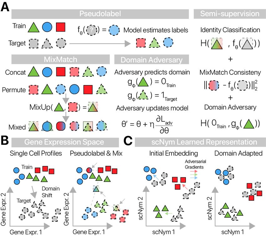
Downloaded from genome.cshlp.org on April 17, 2021 - Published by Cold Spring Harbor Laboratory Press
65 type classification error on these mixed profiles, encouraging the model to learn a general representation that allows for
66 interpolation between observed cell states.
67 The scNym classifier learns a representation of cell identity in the hidden neural network layers where cell types are
68 linearly separable. Alongside, we train an adversarial model to predict the domain-of-origin for each cell (e.g. training
69 set, target set) from this learned embedding. We train the scNym classifier to compete with this adversary, updating the
70 classifier’s embedding to make domain prediction more difficult. At each iteration, the adversary’s gradients highlight
71 features in the embedding that discriminate the different domains. We update the scNym classifier using the inverse of
72 the adversarial gradients, reducing the amount of domain-specific information in the embedding as training progresses.
73 This adversarial training procedure encourages the classification model to learn a domain-adapted embedding of the
74 training and target datasets that improves classification performance (Fig. 1C). In inference mode, scNym predictions
75 provide a probability distribution across all cell types in the training set for each target cell.
76 scNym transfers cell annotations across biological conditions
77 We evaluated the performance of scNym transferring cell identity annotations in eleven distinct tasks. These tasks were
78 chosen to capture diverse kinds of technological and biological variation that complicate annotation transfer. Each task
79 represents a true cell type transfer across different experiments, in contrast to some efforts that report within-experiment
80 hold-out accuracy.
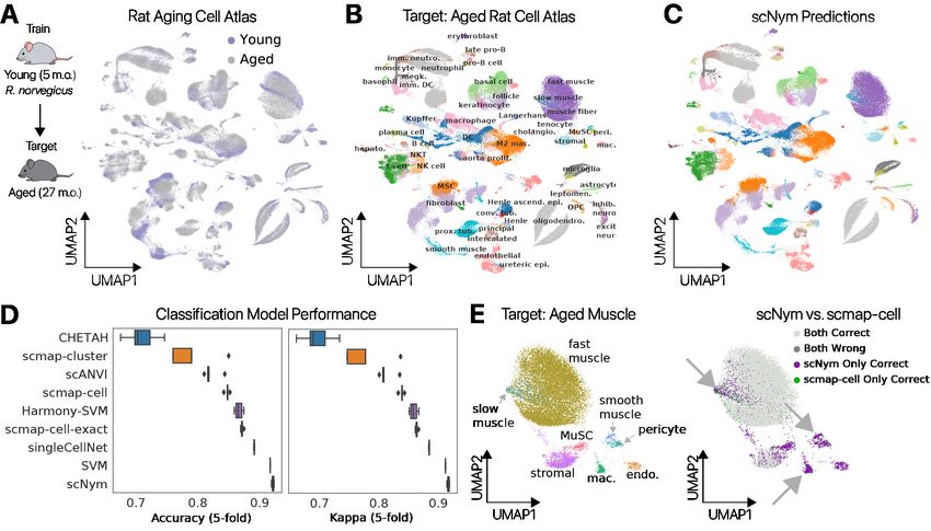
81 We first evaluated cell type annotation transfer between animals of different ages. We trained scNym models on cells
82 from young rats (5 months old) from the Rat Aging Cell Atlas [Ma et al., 2020] and predicted on cells from aged rats
83 (27 months old, Fig. 2A, Methods). We found that predictions from our scNym model trained on young cells largely
84 matched the ground truth annotations (92.2% accurate) on aged cells (Fig. 2B, C).
85 We compared scNym performance on this task to state of the art single cell identity annotation meth-
86 ods [Kiselev et al., 2018, Alquicira-Hernandez et al., 2019, Tan and Cahan, 2019, Abdelaal et al., 2019,
87 de Kanter et al., 2019]. We also compared scNym to state of the art unsupervised data harmonization meth-
88 ods [Korsunsky et al., 2019, Stuart et al., 2019, Xu et al., 2019, Tran et al., 2020] followed by supervised classification
89 with a support vector machine, for a total of ten baseline approaches (Methods). scNym produced significantly
90 improved labels over these methods, some of which could not complete this large task on our hardware (256GB RAM)
91 (Wilcoxon Rank Sums on accuracy or -scores, p < 0.01, Fig. 2D, Table 1). scNym runtimes were competitive
92 with baseline methods (Fig. S1). We found that some of the largest differences in accuracy between scNym and the
93 commonly used scmap-cell method were in the skeletal muscle. scNym models accurately classified multiple cell
94 types in the muscle that were confused by scmap-cell (Fig. 2E), demonstrating that the increased accuracy of scNym is
95 meaningful for downstream analyses.
96 We next tested the ability of scNym to classify cell identities after perturbation. We trained on unstimulated
97 human peripheral blood mononuclear cells (PBMCs) and predicted on PBMCs after stimulation with IFNB1
4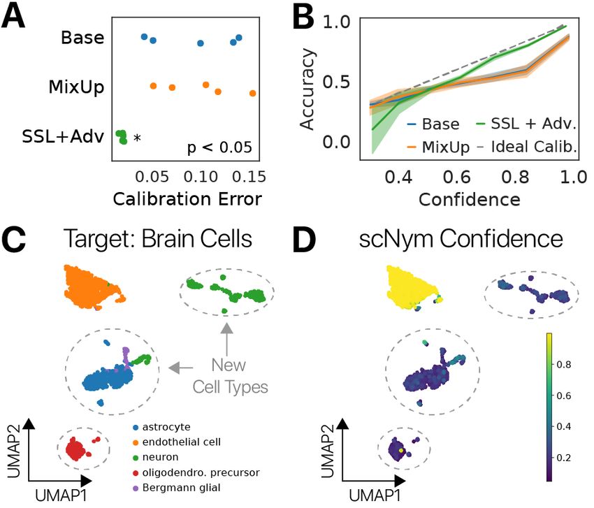
Downloaded from genome.cshlp.org on April 17, 2021 - Published by Cold Spring Harbor Laboratory Press

98    (Fig. 3A)[Kang et al., 2017]. scNym achieved high accuracy (> 91%), superior to baseline methods (Fig. 3C, Table 1).
99    The common scmap-cluster method frequently confused monocyte subtypes, while scNym did not (Fig. 3B).

100   Cross-species annotation transfer is another context where distinct biology creates a domain shift across training and
101   target domains. To evaluate if scNym could transfer labels across species, we trained on mouse cells with either rat or
102   human cells as target data and observed high performance (Fig. S2).

103   scNym models learn biologically meaningful cell type representations

104   To interpret the classification decisions of our scNym models, we developed integrated gradient analysis tools to identify
105   genes that influence model decisions (Methods)[Sundararajan et al., 2017]. The integrated gradient method attributes
106   the prediction of a deep network to its input features, while satisfying desirable axioms of interpretability that simpler
107   methods like raw gradients do not. For the PBMC cross-stimulation task, we found that salient genes included known
108   markers of specific cell types such as CD79A for B cells and GNLY for NK cells. Integrated gradient analysis also
109   revealed specific cell type marker genes that may not have been selected a priori, such as NCOA4 for megakaryocytes
110   (Fig. 3D, E, Fig. S3). We also performed integrated gradient analysis for a cross-technology mouse cell atlas experiment
111   (described below) and found that marker genes chosen using scNym integrated gradients were superior to markers
112   chosen using SVM feature importance scores based on Gene Ontology enrichment (Fig. S4). These results suggest
113   that our models learned biologically meaningful representations that are more generalizable to unseen cell profiles,
114   regardless of condition or technology.

115   We also used integrated gradient analysis to understand why the scNym model misclassified some FCGR3A+ monocytes
116   as CD14+ monocytes in the PBMC cross-stimulation task (Methods). This analysis revealed genes driving these
117   incorrect classifications, including some CD14+ monocyte marker genes that are elevated in a subset of FCGR3A+
118   monocytes (Fig. 3F). Domain experts may use integrated gradient analysis to understand and review model decisions
119   for ambiguous cells.

120   scNym transfers annotations across single cell sequencing technologies

121   To evaluate the ability of scNym to transfer labels across different experimental technologies, we trained on single
122   cell profiles from ten mouse tissues in the Tabula Muris captured using the 10x Chromium technology and predicted
123   labels for cells from the same compendium captured using Smart-seq2 [Tabula Muris Consortium, 2018]. We found
124   that scNym predictions were highly accurate (> 90%) and superior to baseline methods (Fig. S5A, B, C). scNym
125   models accurately classified monocyte subtypes, while baseline methods frequently confused these cells (Fig. S5D, E).

126   In a second cross-technology task, we trained scNym on mouse lung data from the Tabula Muris and predicted on lung
127   data from the Mouse Cell Atlas, a separate experimental effort that used the Microwell-seq technology [Han et al., 2018].
128   We found that scNym yielded high classification accuracy (> 90%), superior to baseline methods, despite experimental
129   batch effects and differences in the sequencing technologies (Fig. S6). We also trained scNym models to transfer

                                                                  5
Downloaded from genome.cshlp.org on April 17, 2021 - Published by Cold Spring Harbor Laboratory Press
130 regional identity annotations in spatial transcriptomics data and found performance competitive with baseline methods
131 (Fig. S7). Together, these results demonstrate that scNym models can effectively transfer cell type annotations across
132 technologies and experimental environments.
133 Multi-domain training allows integration of multiple reference datasets
134 The number of public single cell datasets is increasing rapidly [Svensson et al., 2018]. Integrating information across
135 multiple reference datasets may improve annotation transfer performance on challenging tasks. The domain adversarial
136 training framework in scNym naturally extends to training across multiple reference datasets. We hypothesized that
137 a multi-domain training approach would allow for more general representations that improve annotation transfer.
138 To test this hypothesis, we evaluated the performance of scNym to transfer annotations between single cell and
139 single nucleus RNA-seq experiments in the mouse kidney. These data contained six different single cell preparation
140 methods and three different single nucleus methods, capturing a range of technical variation in nine distinct domains
141 [Denisenko et al., 2020](Fig. 4A, B).
142 scNym achieved significantly greater accuracy than baseline methods transferring labels from single nucleus to single
143 cell experiments using multi-domain training. This result was also achieved for the inverse transfer task, transferring
144 annotations from single cell to single nucleus experiments (tied with best baseline, Fig. 4C, Table 1). We found
145 that scNym delivered more accurate annotations for multiple cell types in the cell to nucleus transfer task, including
146 mesangial cells and tubule cell types (Fig. 4D, E). These improved annotations highlight that the performance advantages
147 of scNym are meaningful for downstream analysis and biological interpretation. We found that multi-domain scNym
148 models achieved greater accuracy than any single domain model on both tasks and effectively synthesized information
149 from single domain training sets of varying quality (Fig. 4F, Fig. S8). We performed a similar experiment using data
150 from mouse cortex nuclei profiled with four distinct single cell sequencing methods, training on three methods at a time
151 and predicting annotations for the held-out fourth method for a total of four unique tasks. scNym was the top ranked
152 method across tasks (Fig. S9).
153 scNym confidence scores enable expert review and allow new cell type discoveries
154 Calibrated predictions, in which the classification probability returned by the model precisely reflects the probability it
155 is correct, enable more effective interaction of the human researcher with the model output. We investigated scNym
156 calibration by comparing the prediction confidence scores to prediction accuracy (Methods). We found that semi-
157 supervised adversarial training improved model calibration, such that high confidence predictions are more likely to be
158 correct (Fig. 5A, B; Fig. S10A, B; Fig. S11). scNym confidence scores can therefore be used to highlight cells that
159 may benefit from manual review (Fig. S10C, Fig. S11B), further improving the annotation exercise when it contains a
160 domain expert in the loop.
161 scNym confidence scores can also highlight new, unseen cell types in the target dataset using an optional pseudolabel
162 thresholding procedure during training, inspired by FixMatch [Sohn et al., 2020] (Methods). The semi-supervised
6Downloaded from genome.cshlp.org on April 17, 2021 - Published by Cold Spring Harbor Laboratory Press
163 and adversarial components of scNym encourage the model to find a matching identity for cells in the target dataset.
164 Pseudolabel thresholding allows scNym to exclude cells with low confidence pseudolabels from the semi-supervised
165 and adversarial components of training, stopping these components from mismatching unseen cell types and resulting
166 in correctly uncertain predictions.
167 To test this approach, we simulated two experiments where we “discover” multiple cell types by predicting annotations
168 on the Tabula Muris brain cell data using models trained on non-brain tissues (Fig. 5A, B; Methods). We first used
169 pre-trained scNym models to predict labels for new cell types not present in the original training or target sets, and
170 scNym correctly marked these cells with low confidence scores (Fig. S12). In the second experiment, we included
171 new cell types in the target set during training and found that scNym models with pseudolabel thresholding correctly
172 provided low confidence scores to new cell types, highlighting these cells as potential cell type discoveries for manual
173 inspection (Fig. 5C, D; Fig. S13).
174 We found that scNym embeddings capture cell type differences even within the low confidence cell population, such
175 that clustering these cells in the scNym embedding can provide a hypothesis for how many new cell types might be
176 present (Fig. S14). We also found that putative new cell types could be discriminated from other low confidence cells,
177 like prediction errors on a cell type boundary (Fig. S15). These results demonstrate that scNym confidence scores can
178 highlight target cell types that were absent in the training data, potentially enabling new cell type discoveries.
179 Semi-supervised and adversarial training components improve annotation transfer
180 We ablated different components of scNym to determine which features were responsible for high performance. We
181 found that semi-supervision with MixMatch and training with a domain adversary improved model performance across
182 multiple tasks (Fig. 6B, Fig. S16). We hypothesized that scNym models might benefit from domain adaptation through
183 the adversarial model by integrating the cells into a latent space more effectively. Supporting this hypothesis, we found
184 that training and target domains were significantly more mixed in scNym embeddings (Fig. S17). These results suggest
185 that semi-supervision and adversarial training improve the accuracy of cell type classifications.
186 scNym is robust to hyperparameter selection
187 Hyperparameter selection can be an important determinant of classification model performance. In all tasks presented
188 here, we have used the same set of default scNym parameters derived from past recommendations in the representation
189 learning literature (Methods). To determine how sensitive scNym performance is to these hyperparameter choices, we
190 trained scNym models on the hPBMC cross-stimulation task across a grid of hyperparameter values. We found that
191 scNym is robust to hyperparameter changes within an order of magnitude of the default values, demonstrating that
192 our defaults are not “overfit” to the benchmark tasks presented here (Fig. S18). We also performed hyperparameter
193 optimization using reverse 5-fold cross-validation for the top three baseline methods (SVM, singleCellNet, scmap-cell-
194 exact) to determine if an optimized baseline was superior to scNym across four benchmarking tasks (Methods). We
7Downloaded from genome.cshlp.org on April 17, 2021 - Published by Cold Spring Harbor Laboratory Press
195 found that scNym performance using default parameters was superior to the performance of baseline methods after
196 hyperparameter tuning (Table S3, Fig. S19).
197 Discussion
198 Single cell genomics experiments have become more accessible due to commercial technologies, enabling a rapid
199 increase in the use of these methods [Svensson et al., 2020]. Cell identity annotation is an essential step in the analysis
200 of these experiments, motivating the development of high performance, automated annotation methods that can take
201 advantage of diverse datasets. Here, we introduced a semi-supervised adversarial neural network model that learns to
202 transfer annotations from one experiment to another, taking advantage of information in both labeled training sets and
203 an unlabeled target dataset.
204 Our benchmark experiments demonstrate that scNym models provide high performance across a range of cell identity
205 classification tasks, including cross-age, cross-perturbation, and cross-technology scenarios. scNym performs better
206 in these varied conditions than ten state of the art baseline methods, including three unsupervised data integration
207 approaches paired with supervised classifiers (Fig. 6A, Table 1). The superiority of scNym is consistent across
208 diverse performance metrics, including accuracy, Cohen’s -score, and the multi-class receiver operating characteristic
209 (MCROC; Fig. S20, Table S1, Table S2).
210 The key idea that differentiates scNym from previous cell classification approaches is the use of semi-supervised
211 [Berthelot et al., 2019] and adversarial training [Ganin et al., 2016] to extract information from the unlabeled, target
212 experiment we wish to annotate. Through ablation experiments, we showed that these training strategies improve the
213 performance of our models. Performance improvements were most pronounced when there were large, systematic
214 differences between the training and target datasets (Fig. 3). Semi-supervision and adversarial training also allow scNym
215 to integrate information across multiple training and target datasets, improving performance (Fig. 4). As large scale
216 single cell perturbation experiments become more common [Dixit et al., 2016, Srivatsan et al., 2019] and multiple cell
217 atlases are released for common model systems, our method’s ability to adapt across distinct biological and technical
218 conditions will only increase in value.
219 Most downstream biological analyses rely upon cell identity annotations, so it is important that researchers are able to
220 interpret the molecular features that drive model decisions. We showed that backpropagation-based saliency analysis
221 methods are able to recover specific cell type markers, confirming that scNym models learn interpretable, biologically
222 relevant features of cell type. In future work, we hope to extend upon these interpretability methods to infer perturbations
223 that alter cell identity programs using the informative representations learned by scNym.
8Downloaded from genome.cshlp.org on April 17, 2021 - Published by Cold Spring Harbor Laboratory Press
224 Methods
225 scNym Model
226 Our scNym model f✓ consists of a neural network with an input layer, two hidden layers, each with 256 nodes, and an out-
227 put layer with a node for each class. The first three layers are paired with batch normalization [Ioffe and Szegedy, 2015],
228 rectified linear unit activation, and dropout [Srivastava et al., 2014]. The final layer is paired with a softmax activation
229 to transform real number outputs of the neural network into a vector of class probabilities. The model maps cell profile
230 vectors x to probability distributions p(y|x) over cell identity classes y.
p(y|x) = f✓ (x)
231 We train scNym to map cell profiles in a gene expression matrix x 2 XCells⇥Genes to paired cell identity annotations
232 y 2 y. Transcript counts in the gene expression matrix are normalized to counts per million (CPM) and log-transformed
233 after addition of a pseudocount (log(CPM + 1)). During training, we randomly mask 10% of genes in each cell with 0
234 values, then renormalize to obtain an augmented profile.
235 We use the Adadelta adaptive stochastic gradient descent method [Zeiler, 2012] with an initial learning rate of ⌘ = 1.0 to
236 update model parameters on minibatches of cells, with batch sizes of 256. We apply a weight decay term of WD = 10 4
237 for regularization. We train scNym models to minimize a standard cross-entropy loss function for supervised training.
" K
#
X
LCE (X, f✓ ) = E(x,y)⇠(X,y) y(k) log(f✓ (x))k
k=1
238 where y(k) is an indicator variable for the membership of x in class k, and k 2 K represent class indicators.
239 We fit all scNym models for a maximum of 400 epochs and selected the optimal set of weights using early stopping on
240 a validation set consisting of 10% of the training data. We initiate early stopping after training has completed at least
241 5% of the total epochs to avoid premature termination.
242 Prior to passing each minibatch to the network, we perform dynamic data augmentation with the “MixUp” operation
243 [Zhang et al., 2018]. MixUp computes a weighted average of two samples x and x0 where the weights are randomly
244 sampled from a Beta distribution with a symmetric shape parameter ↵.
Mix (x, x0 ) = x + (1 )x0 ; ⇠ Beta(↵, ↵)
245 For all experiments here, we set ↵ = 0.3 based on performance in the natural image domain [Zhang et al., 2018].
246 Forcing models to interpolate predictions smoothly between samples shifts the decision boundary away from high-
247 density regions of the input distribution, improving generalization. This procedure has been shown to improve classifier
9Downloaded from genome.cshlp.org on April 17, 2021 - Published by Cold Spring Harbor Laboratory Press
248 performance on multiple tasks [Zhang et al., 2018]. Model calibration – the correctness of a model’s confidence scores
249 for each class – is generally also improved by this augmentation scheme [Thulasidasan et al., 2019].
250 Semi-supervision with MixMatch
251 We train semi-supervised scNym models using the MixMatch framework [Berthelot et al., 2019], treating the target
252 dataset as unlabeled data U . At each iteration, MixMatch samples minibatches from both the labeled dataset (X, y) ⇠ D
253 and unlabeled dataset U ⇠ U. We generate “pseudolabels” [Lee, 2013] using model predictions for each observation in
254 the unlabeled minibatch (Supplemental Methods).
ui ⇠ U; zi = f✓ (ui )
255 We next “sharpen” the pseudolabels using a “temperature scaling” procedure [Hinton et al., 2015, Guo et al., 2017]
256 with the temperature parameter T = 0.5 as a form of entropy minimization (Supplemental Methods). This entropy
257 minimization encourages unlabeled examples to belong to one of the described classes.
258 We then randomly mix each observation and label/pseudolabel pair in both the labeled and unlabeled minibatches with
259 another observation using MixUp [Zhang et al., 2018]. We allow labeled and unlabeled observations to mix together
260 during this procedure (Supplemental Methods).
⇠ Beta(↵, ↵)
261
wm = Mix (wi , wj ); qm = Mix (qi , qj )
262 where (wi , qi ) is either a labeled observation and ground truth label (xi , yi ) or an unlabeled observation and the
263 pseudolabel (ui , zi ). This procedure yields a minibatch X0 of mixed labeled observations and a minibatch U0 of mixed
264 unlabeled observations.
265 We introduce a semi-supervised interpolation consistency penalty during training in addition to the standard supervised
266 loss. For observations and pseudolabels in the mixed unlabeled minibatch U 0 , we penalize the mean squared error
267 (MSE) between the mixed pseudolabels and the model prediction for the mixed observation (Supplemental Methods).
LSSL (U0 , f✓ ) = Eum ,zm ⇠U0 kf✓ (um ) zm k22
268 This encourages the model to provide smooth interpolations between observations and their ground truth or pseudolabels,
269 generalizing the decision boundary of the model. We weight this unsupervised loss relative to the supervised cross-
270 entropy loss using a weighting function SSL (t) ! [0, 1]. We initialize this coefficient to SSL = 0 and increase the
271 weight to a final value of SSL = 1 over 100 epochs using a sigmoid schedule (Supplemental Methods).
10Downloaded from genome.cshlp.org on April 17, 2021 - Published by Cold Spring Harbor Laboratory Press
L(X0 , U0 , f✓ , t) = LCE (X0 , f✓ ) + SSL (t)LSSL (U
0
, f✓ )
272 Domain Adaptation with Domain Adversarial Networks
273 We use domain adversarial networks (DAN) as an additional approach to incorporate information from the target
274 dataset during training [Ganin et al., 2016]. The DAN method encourages the classification model to embed cells from
275 the training and target dataset with similar coordinates, such that training and target datasets are well-mixed in the
276 embedding. By encouraging the training and target dataset to be well-mixed, we take advantage of the inductive bias that
277 cell identity classes in each dataset are similar, despite technical variation or differences in conditions (Supplemental
278 Methods).
279 We introduce this technique into scNym by adding an adversarial domain classification network g . We implement g
280 as a two-layer neural network with a single hidden layer of 256 units and a rectified linear unit activation, followed by a
281 classification layer with two outputs and a softmax activation. This adversary attempts to predict the domain of origin d
282 from the penultimate classifier embedding v of each observation. For each forward pass, it outputs a probability vector
283 dˆ estimating the likelihood the observation came from the training or target domain.
284 We assign a one-hot encoded domain label d to each molecular profile based on the experiment of origin (Supplemental
285 Methods). During training, we pass a minibatch of labeled observations x 2 X and unlabeled observations u 2 U
286 through the domain adversary to predict domain labels.
dˆ = g (v) = g (f✓ (x)(l 1)
)
287 where dˆ is the domain probability vector and v = f✓ (x)(l 1)
denotes the embedding of x from the penultimate layer of
288 the classification model f✓ . We fit the adversary using a multi-class cross-entropy loss, as described above for the main
289 classification loss (Supplemental Methods).
290 To make use of the adversary for training the classification model, we use the “gradient reversal” trick at each backward
291 pass. We update the parameters of the adversary using standard gradient descent on the loss Ladv . At each backward
292 pass, this optimization improves the adversarial domain classifier (Supplemental Methods). We update the parameters ✓
293 of the classification model using the inverse of the gradients computed during a backward pass from Ladv . Using the
294 inverse gradients encourages the classification model f✓ to generate an embedding where it is difficult for the adversary
295 to predict the domain (Supplemental Methods). Our update rule for the classification model parameters therefore
296 becomes:
✓ ◆
@LCE @LSSL @Ladv
✓t = ✓t 1 ⌘ + SSL (t) adv (t)
@✓ @✓ @✓
11Downloaded from genome.cshlp.org on April 17, 2021 - Published by Cold Spring Harbor Laboratory Press
297 We increase the weight of the adversary gradients from adv ! [0, 0.1] over the course of 20 epochs during training
298 using a sigmoid schedule. We scale the adversarial gradients flowing to ✓, rather than the adversarial loss term, so that
299 full magnitude gradients are used to train a robust adversary g (Supplemental Methods). Incorporating both MixMatch
300 and the domain adversary, our full loss function becomes:
L(X, U, X0 , U0 , f✓ , g , t) = LCE (X0 , f✓ ) + SSL (t)LSSL (U
0
, f✓ ) + Ladv (X, U, f✓ , g , t)
301 Pseudolabel Thresholding for New Cell Type Discovery
302 Entropy minimization and domain adversarial training enforce an inductive bias that all cells in the target dataset belong
303 to a class in the training dataset. For many cell type classification tasks, this assumption is valid and useful. However, it
304 is violated in the case where new, unseen cell types are present in the target dataset. We introduce an alternative training
305 configuration to allow for quantitative identification of new cell types in these instances.
306 We have observed that new cell types will receive low confidence pseudolabels, as they do not closely resemble any
307 of the classes in the training set (Fig. S12). We wish to exclude these low confidence pseudolabels from our entropy
308 minimization and domain adversarial training procedures, as these methods both incorrectly encourage these new cell
309 types to receive high confidence predictions and embeddings for a known cell type. We therefore adopt a notion of
310 “pseudolabel confidence thresholding” introduced in the FixMatch method [Sohn et al., 2020]. To identify confident
311 pseudolabels to use during training, we set a minimum pseudolabel confidence ⌧ = 0.9 and assign all pseudolabels a
312 binary confidence indicator ci 2 {0, 1} (Supplemental Methods).
313 We make two modifications to the training procedure to prevent low confidence pseudolabels from contributing to
314 any component of the loss function. First, we use only high confidence pseudolabels in the MixUp operation of the
315 MixMatch procedure. This prevents low confidence pseudolabels from contributing to the supervised classification
316 or interpolation consistency losses (Supplemental Methods). Second, we use only unlabeled examples with high
317 confidence pseudolabels to train the domain adversary. These low confidence unlabeled examples can therefore occupy
318 a unique region in the model embedding, even if they are easily discriminated from training examples. Our adversarial
319 loss is slightly modified to penalize domain predictions only on confident samples in the pseudolabeled minibatch
320 (Supplemental Methods).
321 We found that this pseudolabel thresholding configuration option was essential to provide accurate, quantitative
322 information about the presence of new cell types in the target dataset (Fig. S13). However, this option does modestly
323 decrease performance when new cell types are not present. We therefore enable this option when the possibility of new
324 cell types violates the assumption that the training and target data share the same set of cell types. We have provided a
325 simple toggle in our software implementation to allow users to enable or disable this feature.
12Downloaded from genome.cshlp.org on April 17, 2021 - Published by Cold Spring Harbor Laboratory Press
326 scNym Model Embeddings
327 We generate gene expression embeddings from our scNym model by extracting the activations of the penultimate neural
328 network layer for each cell. We visualize these embeddings using UMAP [McInnes et al., 2020, Becht et al., 2018] by
329 constructing a nearest neighbor graph (k = 30) in principal component space derived from the penultimate activations.
330 We set min_dist = 0.3 for the UMAP minimum distance parameter.
331 We present single cell experiments using a 2-dimensional representation fit using the UMAP alogrithm
332 [Becht et al., 2018]. For each experiment, we compute a PCA projection on a set of highly variable genes after
333 log(CPM + 1) normalization. We construct a nearest neighbor graph using first 50 principal components and fit a
334 UMAP projection from this nearest neighbor graph.
335 Entropy of Mixing
336 We compute the “entropy of mixing” to determine the degree of domain adaptation between training and target datasets
337 in an embedding X. The entropy of mixing is defined as the entropy of a vector of class membership in a local
338 neighborhood of the embedding:
K
X
Local
H(p )= pLocal
k log pLocal
k
k=1
339 where pLocal is a vector of class proportions in a local neighborhood and k 2 K are class indices. We compute the
340 entropy of mixing for an embedding X by randomly sampling n = 1000 cells, and computing the entropy of mixing on
341 a vector of class proportions for the 100 nearest neighbors to each point.
342 Integrated Gradient Analysis
343 We interpreted the predictions of our scNym models by performing integrated gradient analysis
344 [Sundararajan et al., 2017]. Given a trained model f✓ and a target class k, we computed an integrated gradi-
345 ent score IG as the sum of gradients on a class probability f✓ (x)k with respect to an input gene expression vector x at
346 M = 100 points along a linear path between the zero vector and the input x. We then multiplied the sum of gradients
347 for each gene by the expression values in the input x. Stated formally, we computed:
M
1 X @f✓ ( M
m
x)k
IG(x, k, f✓ ) = x ·
M m=1 @x
348 In the original integrated gradient formalism, this is equivalent to using the zero vector as a baseline. We average the
349 integrated gradients across ns cell input vectors x to obtain class-level maps IGk , where ns = min(300, nk ) and nk is
350 the number of cells in the target class. To identify genes that drive incorrect classifications, we computed integrated
351 gradients with respect to some class k for cells with true class k 0 that were incorrectly classified as class k.
13Downloaded from genome.cshlp.org on April 17, 2021 - Published by Cold Spring Harbor Laboratory Press
352 Interpretability Comparison
353 We compared the biological relevance of features selected by scNym and SVM as a baseline by computing cell type
354 specific Gene Ontology enrichments. We trained both scNym and an SVM to transfer labels from the Tabula Muris
355 10x Genomics dataset to the Tabula Muris Smart-seq2 dataset. We then extracted feature importance scores from the
356 scNym model using integrated gradients and from the SVM model based on coefficient weights. We selected cell type
357 markers for each model as the top k = 100 genes with the highest integrated gradient values or SVM coefficients.
358 For 19 cell types with corresponding Gene Ontology terms, we computed the enrichment of the relevant cell type specific
359 Gene Ontology terms in scNym-derived and SVM-derived cell type markers using Fischer’s exact test (Supplemental
360 Methods). We present a sample of the gene sets used (Table S4). We compared the mean Odds-Ratio from Fischer’s
361 exact test across relevant Gene Ontology terms between scNym-derived markers and SVM-derived markers. To
362 determine statistical significance of a difference in these mean Odds-Ratios, we performed a paired t-test across cell
363 types. We performed the procedure above using k 2 {50, 100, 150} to determine the sensitivity of our results to this
364 parameter. We found that scNym integrated gradients had consistently stronger enrichments for relevant Gene Ontology
365 terms across cell types for all values of k.
366 Model Calibration Analysis
367 We evaluated scNym calibration by binning all cells in a query set based on the softmax probability of their assigned
368 class – maxk (softmax(f✓ (x)k )) – which we term the “confidence score”. We grouped cells into M = 10 bins Bm of
369 equal width from [0, 1] and computed the mean accuracy of predictions within each bin.
acc(Bm ) = h (ŷ ⌘ y)i
conf(Bm ) = hmax p̂i i
370 where (a ⌘ b) denotes a binary equivalency operation that yields 1 if a and b are equivalent and 0 otherwise and h·i
371 denotes the arithmetic average.
372 We computed the “expected calibration error” as previously proposed [Thulasidasan et al., 2019].
XM
|Bm |
ECE = |acc(Bm ) conf(Bm )|
m=1
N
373 We also computed the “overconfidence error”, which specifically focuses on high confidence but incorrect predictions.
oe(Bm ) = conf(Bm ) max ((conf(Bm ) acc(Bm )), 0)
14Downloaded from genome.cshlp.org on April 17, 2021 - Published by Cold Spring Harbor Laboratory Press
374
XM
|Bm |
OE = oe(Bm )
m=1
N
375 where N is the total number of samples, and |Bm | is the number of samples in bin Bm .
376 We performed this analysis for each model trained in a 5-fold cross-validation split to estimate calibration for a given
377 model configuration. We evaluated calibrations for baseline neural network models, models with MixUp but not
378 MixMatch, and models with the full MixMatch procedure.
379 Baseline Methods
380 As baseline methods, we used ten cell identity classifiers: scmap-cell, scmap-cluster [Kiselev et al., 2018,
381 Andrews and Hemberg, 2018], scmap-cell-exact (scmap-cell with exact k-NN search), a linear SVM
382 [Abdelaal et al., 2019], scPred [Alquicira-Hernandez et al., 2019], singleCellNet [Tan and Cahan, 2019], CHETAH
383 [de Kanter et al., 2019], Harmony followed by an SVM [Korsunsky et al., 2019], LIGER followed by an SVM
384 [Stuart et al., 2019], and scANVI [Lopez et al., 2018, Xu et al., 2019]. For model training, we split data into 5-folds
385 and trained five separate models, each using 4 folds for training and validation data. This allowed us to assess variation
386 in model performance as a function of changes in the training data. No class balancing was performed prior to training,
387 though some methods perform class balancing internally. All models, including scNym, were trained on the same
388 5-fold splits to ensure equitable access to information. All methods were run with the best hyperparameters suggested
389 by the authors unless otherwise stated for our hyperparameter optimization comparisons (full details in Supplemental
390 Methods).
391 We applied all baseline methods to all benchmarking tasks. If a method could not complete the task given 256 GB
392 of RAM and 8 CPU cores, we reported the accuracy for that method as “Undetermined.” Only scNym and scANVI
393 models required GPU resources. We trained models on Nvidia K80, GTX1080ti, Titan RTX, or RTX 8000 GPUs, using
394 only a single GPU per model.
395 Performance Benchmarking
396 For all benchmarks, we computed the mean accuracy across cells (“Accuracy”), Cohen’s -score, and the multiclass
397 recevier operating characteristic (MCROC). We computed the MCROC as the mean of ROC scores across cell types,
398 treating each cell type as a binary classification problem. We performed quality control filtering and pre-processing on
399 each dataset before training (Supplemental Methods).
400 For the Rat Aging Cell Atlas [Ma et al., 2020] benchmark, we trained scNym models on single cell RNA-seq from
401 young, ad libitum fed rats (5 months old) and predicted on cells from aged rats (ad libitum fed or calorically-restricted).
402 For the human PBMC stimulation benchmark, we trained models on unstimulated PBMCs collected from multiple
403 human donors and predicted on IFNB1 stimulated PBMCs collected in the same experiment [Kang et al., 2017].
15Downloaded from genome.cshlp.org on April 17, 2021 - Published by Cold Spring Harbor Laboratory Press
404 For the Tabula Muris cross-technology benchmark, we trained models on Tabula Muris 10x Genomics Chromium
405 platform and predicted on data generated using Smart-seq2. For the Mouse Cell Atlas (MCA) [Han et al., 2018]
406 benchmark, we trained models on single cell RNA-seq from lung tissue in the Tabula Muris 10x Chromium data
407 [Tabula Muris Consortium, 2018] and predicted on MCA lung data. For the spatial transcriptomics benchmark, we
408 trained models on spatial transcriptomics from a mouse sagittal-posterior brain section and predicted labels for another
409 brain section (data downloaded from https://www.10xgenomics.com/resources/datasets/.
410 For the single cell to single nucleus benchmark in the mouse kidney, we trained scNym models on all single
411 cell data from six unique sequencing protocols and predicted labels for single nuclei from three unique protocols
412 [Denisenko et al., 2020]. For the single nucleus to single cell benchmark, we inverted the training and target datasets
413 above to train on the nuclei datasets and predict on the single cell datasets. We set unique domain labels for each
414 protocol during training in both benchmark experiments. To evaluate the impact of multi-domain training, we also
415 trained models on only one single cell or single nucleus protocol using the domains from the opposite technology as
416 target data.
417 For the multi-domain cross-technology benchmark in mouse cortex nuclei, we generated four distinct subtasks from
418 data generated using four distinct technologies to profile the same samples [Ding et al., 2020]. We trained scNym and
419 baseline methods to predict labels on one technology given the remaining three technologies as training data for all
420 possible combinations. We used each technology as a unique domain label for scNym.
421 For the cross-species mouse to rat demonstration, we selected a set of cell types with comparable annotations in the
422 Tabula Muris and Rat Aging Cell Atlas [Ma et al., 2020] to allow for quantitative evaluation. We trained scNym with
423 mouse data as the source domain and rat data as the target domain. We used the new identity discovery configuration
424 to account for the potential for new cell types in a cross-species experiment. For the cross-species mouse to human
425 demonstration, we similarly selected a set of cell types with comparable cell annotation ontologies in the Tabula Muris
426 l0x lung data and human lung cells from the IPF Cell Atlas [Habermann et al., 2020]. We trained an scNym model
427 using mouse data as the source domain and human data as the target, as for the mouse to rat demonstration.
428 Runtime Benchmarking
429 We measured the runtime of scNym and each baseline classification method using subsamples from the multi-domain
430 kidney single cell and single nuclei dataset [Denisenko et al., 2020]. We measured runtimes for annotation transfer
431 from single cells to single nuclei labels using subsamples of size n 2 {1250, 2500, 5000, 10000, 20000, 40000} for
432 each of the training and target datasets. All methods were run on four cores of a 2.1 GHz Intel Xeon Gold 6130 CPU
433 and 64 GB of CPU memory. GPU capable methods (scNym, scANVI) were provided with one Nvidia Titan RTX GPU
434 (consumer grade CUDA compute device).
16Downloaded from genome.cshlp.org on April 17, 2021 - Published by Cold Spring Harbor Laboratory Press
435 Hyperparameter Optimization Experiments
436 We performed hyperparameter optimization across four tasks for the top three baseline methods, the SVM, singleCellNet,
437 and scmap-cell-exact. For the SVM, we optimized the regularization strength parameter C at 12 values (C 2 10k 8k 2
438 [ 6, 5]) with and without class weighting. For class weighting, we set class weights as either uniform or inversely
439 proportional to the number of cells in each class to enforce class balancing (wk = 1/nk , where wk is the weight for class
440 k and nk is the number of cells for that class). For scmap-cell-exact, we optimized (1) the number of nearest neighbors
441 (k 2 {5, 10, 30, 50, 100}), (2) the distance metric (d(·, ·) 2 {cosine, euclidean}), and (3) the number of features to
442 select with M3Drop (nf 2 {500, 1000, 2000, 5000}). For singleCellNet, we optimized with nTopGenes 2 {10, 20},
443 nRand 2 {35, 70, 140}, nTrees 2 {100, 1000, 2000}, and nTopGenePairs 2 {12, 25}.
444 We optimized scNym for two of the four tasks, due to computational expense and superiority of default parameters
445 relative to baseline methods. For scNym, we optimized (1) weight decay ( w 2 10 5
, 10 4
, 10 3
), (2) batch
446 size (M 2 {128, 256}), (3) the number of hidden units (h 2 {256, 512}), (4) the maximum MixMatch weight
447 ( SSL 2 {0.01, 0.1, 1.0}), and (5) the maximum DAN weight ( Adv 2 {0.01, 0.1, 0.2}). We did not optimize weight
448 decay for the PBMC cross-stimulation task. We performed a grid search for all methods.
449 Hyperparameter optimization is non-trivial in the context of a domain shift between the training and test set. Traditional
450 optimization using cross-validation on the training set alone may overfit parameters to the training domain, leading to
451 suboptimal outcomes. This failure mode is especially problematic for domain adaptation models, where decreasing the
452 strength of domain adaptation regularizers may improve performance within the training data, while actually decreasing
453 performance on the target data.
454 In light of these concerns, we adopted a procedure known as reverse cross-validation to evaluate each hyperparameter
455 set [Zhong et al., 2010]. Reverse cross-validation uses both the training and target datasets during training to account
456 for the effect of hyperparameters on the effectiveness of transferring labels across domains. Formally, we first split
457 the labeled training data D into a training set, validation set, and held-out test set D0 , Dv , D⇤ . We use 10% of the
458 training dataset for the validation set and 10% for the held-out test set. We then train a model f✓ : x ! ŷ to transfer
459 labels from the training set D0 to the target data U . We use the validation set Dv for early stopping with scNym and
460 concatenate it into the training set for other methods that do not use a validation set. We treat the predictions ŷ = f✓ (u)
461 as pseudolabels for the unlabeled dataset and subsequently train a second model f : u ! ỹ to transfer annotations
462 from the “pseudolabeled” dataset U back to the labeled dataset D. We then evaluate the “reverse accuracy” as the
463 accuracy of the labels ỹ for the held-out test portion of the labeled dataset, D⇤ .
464 We performed this procedure using a standard 5-fold split for each parameter set. We computed the mean reverse
465 cross-validation accuracy as the performance metric for robustness. For each method that we optimized, we selected the
466 optimal set of hyperparameters as the set with the top reverse cross-validation accuracy.
17Downloaded from genome.cshlp.org on April 17, 2021 - Published by Cold Spring Harbor Laboratory Press
467 New Cell Type Discovery Experiments
468 New Cell Type Discovery with Pre-trained Models
469 We evaluated the ability of scNym to highlight new cell types, unseen in the training data by predicting cell type
470 annotations in the Tabula Muris brain data (Smart-seq2) using models trained on the 10x Genomics data from the ten
471 tissues noted above with the Smart-seq2 data as corresponding target dataset. No neurons or glia were present in the
472 training or target set for this experiment. This experiment simulates the scenario where a pre-trained model has been fit
473 to transfer across technologies (10x to Smart-seq2) and is later used to predict cell types in a new tissue, unseen in the
474 original training or target data.
475 We computed scNym confidence scores for each cell as ci = max pi , where pi is the model prediction probability vector
476 for cell i as noted above. To highlight potential cell type discoveries, we set a simple threshold on these confidence
477 scores di = ci 0.5, where di 2 {0, 1} is a binary indicator variable. We found that scNym assigned low confidence
478 to the majority of cells from newly “discovered” types unseen in the training set using this method.
479 New Cell Type Discovery with Semi-supervised Training
480 We also evaluated the ability of scNym to discover new cell types in a scenario where new cell types are present in
481 the target data used for semi-supervised training. We used the same training data and target data as the experiment
482 above, but we now introduce the Tabula Muris brain data (Smart-seq2) into the target dataset during semi-supervised
483 training. We performed this experiment using our default scNym training procedure, as well as the modified new cell
484 type discovery procedure described above.
485 As above, we computed confidence scores for each cell and set a threshold of di = ci 0.5 to identify potential new
486 cell type discoveries. We found that scNym models trained with the new cell type discovery procedure provided low
487 confidence scores to the new cell types, suitable for identification of these new cells. We considered all new cell type
488 predictions to be incorrect when computing accuracy for the new cell type discovery task.
489 Clustering Candidate New Cell Types
490 We employed a community detection procedure in the scNym embedding to suggest the number of distinct cell
491 states represented by low confidence cells. First, we identify cells with a confidence score lower than a threshold
492 tconf to highlight putative cell type discoveries, di = ci < tconf . We then extract the scNym penultimate embedding
493 activations for these low confidence cells and construct a nearest neighbor graph using the k = 15 nearest neighbors
494 for each cell. We compute a Leiden community detection partition for a range of different resolution parameters
495 r 2 {0.1, 0.2, 0.3, 0.5, 1.0} and compute the Calinski-Harabasz score for each partition [Calinski and Harabasz, 1974].
496 We select the optimal partition in the scNym embedding as the partition generated with the maximum Calinski-Harabasz
497 score and suggest that communities in this partition may each represent a distinct cell state.
18Downloaded from genome.cshlp.org on April 17, 2021 - Published by Cold Spring Harbor Laboratory Press
498 Discriminating Candidate New Cell Types from Other Low Confidence Predictions
499 Cells may receive low confidence predictions for multiple reasons, including: (1) a cell is on the boundary between two
500 cell types, (2) a cell has very little training data for the predicted class, and (3) the cell represents a new cell type unseen
501 in the training dataset. To discriminate between these possibilities, we employ a heuristic similar to the one we use for
502 proposing a number of new cell types that might be present. First, we extract the scNym embedding coordinates from
503 the penultimate layer activations for all cells and build a nearest neighbor graph. We then optimize a Leiden cluster
504 partition by scanning different resolution parameters to maximize the Calinksi-Harabasz score. We then compute the
505 average prediction confidence across all cells in each of the resulting clusters. We also visualize the number of cells
506 present in the training data for each predicted cell type.
507 We consider cells with low prediction scores within an otherwise high confidence cluster to be on the boundary between
508 cell types. These cells may benefit from domain expert review of the specific criteria to use when discriminating
509 between very similar cell identities. We consider low confidence cell clusters with few training examples for the
510 predicted class to warrant further domain expert review. Low confidence clusters that are predicted to be a class with
511 ample training data may represent new cell types and also warrant further review.
512 Software Availability
513 Open source code for our software and pre-processed reference datasets analyzed in this study are available in the
514 scNym repository (https://github.com/calico/scnym) and as Supplemental Code.
515 Competing Interests
516 JCK and DRK are paid employees of Calico Life Sciences, LLC.
517 Acknowledgements
518 JCK conceived the study, implemented software, conducted experiments, and wrote the paper. DRK conceived the
519 study and wrote the paper. We thank Zhenghao Chen, Amoolya H. Singh, and Han Yuan for helpful discussions and
520 comments. Funding for this study was provided by Calico Life Sciences, LLC.
19You can also read