Neural control of computer cursor velocity by decoding motor cortical spiking activity in humans with tetraplegia
←
→
Page content transcription
If your browser does not render page correctly, please read the page content below
1

Neural control of computer cursor velocity by decoding motor

cortical spiking activity in humans with tetraplegia

Sung-Phil Kim1,6 , John D Simeral2,3, Leigh R Hochberg2,3,4, John P Donoghue2,3,5 and Michael
J Black1,6
1
 Department of Computer Science, Brown University, Providence, RI 02911 USA
2
    The Center for Restorative and Regenerative Medicine, Rehabilitation R&D Service, Dept. of Veterans
Affairs, Providence, RI 02912 USA
3
    Department of Neuroscience, Brown University, Providence, RI 02912 USA
4
    Dept. of Neurology, Massachusetts General, Brigham and Women’s, and Spaulding Rehab. Hospitals,
Harvard Medical School, Boston, MA, 02114 USA
5
    Cyberkinetics Neurotechnology Systems, Inc., Foxborough, MA, 02035 USA

E-mail: {spkim, black}@cs.brown.edu

Abstract. Computer-mediated connections between human motor cortical neurons and assistive devices
promise to improve or restore lost function in people with paralysis. Recently, a pilot clinical study of an
intracortical neural interface system demonstrated that a tetraplegic human was able to obtain continuous two-
dimensional control of a computer cursor using neural activity recorded from his motor cortex. This control,
however, was not sufficiently accurate for reliable use in many common computer control tasks.       Here we
studied several central design choices for such a system including the kinematic representation for cursor
movement, the decoding method that translates neuronal ensemble spiking activity into a control signal and
the cursor control task used during training for optimizing the parameters of the decoding method. In two

6
    Address for correspondence: Department of Computer Science, Brown University, Box 1910, 115
Waterman St., Providence, RI 02912, USA

JPD is the Chief Scientific Officer and a director of Cyberkinetics Neurotechnology Systems (CYKN); he
holds stocks and receives compensation. JDS has been a consultant for CYKN. LRH receives clinical trial
support from CYKN.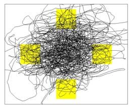
2

tetraplegic participants, we found that controlling a cursor’s velocity resulted in more accurate closed-loop
control than controlling its position directly and that cursor velocity control was achieved more rapidly than
position control.   Control quality was further improved over conventional linear filters by using a
probabilistic method, the Kalman filter, to decode human motor cortical activity.    Performance assessment
based on standard metrics used for evaluation of a wide range of pointing devices demonstrated significantly
improved cursor control with velocity rather than position decoding.

1. Introduction
Injury or disease affecting subcortical, brainstem, spinal, or neuromuscular motor pathways, can
result in paralysis while leaving cerebral function intact.        A neural interface system (NIS) is a
brain-computer interface that provides alternative connections between neurons and assistive
devices and thus has the potential to restore lost function.           Several studies in able-bodied non-
human primates have demonstrated that extracellular neural activity from a population of neurons in
the motor areas of cerebral cortex can be converted into a continuous control signal for the
operation of computers or robotic devices [1-8] (see [9-12] for review). Central to the function of an
NIS is an algorithm for decoding neural activity into a stable, reliable control signal.         In a recent
study, Hochberg et al. [13] demonstrated that paralyzed humans could operate an NIS that
translated motor cortical neural activity into a two-dimensional (2D) computer cursor position.
That report found that neural signals related to movement remained in the arm area of human motor
cortex years after spinal cord injury and that these signals could be activated by imagined or
attempted movement, essential requirements for the operation of an NIS.             Two-dimensional (2D)
cursor control, along with prosthetic hand and robotic arm control, was derived using a linear filter
decoding method that computed 2D cursor position from a linear combination of neural population
firing rates over a short time history [14].
  While demonstrating the ability for a tetraplegic human to control a neural cursor well enough to
operate a simplified computer interface, the quality of cursor control reported in the Hochberg et al.
study [13] was typically not at the level achieved by able-bodied users of standard computer
pointing devices.     In particular, the cursor trajectories were longer and more curved than the
typical straight-line movements of able-bodied users.        Further, it was difficult for the user to stop
the cursor at a target location and to maintain a fixed position. Our goal is to improve NIS function
while shedding light on key issues in the design of any NIS including: 1) the features of intended
movement (e.g. kinematic representation) that are most natural for cursor control; 2) how training of
the neural decoding algorithm affects cursor control accuracy; 3) the statistical stationarity of neural
3

tuning properties between training and testing; 4) quantification of the control accuracy obtained
using different features and decoding algorithms (in terms of cursor trajectory accuracy and target
acquisition rate); and 5) the effect of the choice of decoding algorithm on performance.   For two
participants in our ongoing pilot clinical trial, investigation of each of these issues is described
below.   A central question addressed here is whether cursor position or velocity provides a more
natural movement “feature” for accurate neural cursor control.         Specifically we address this
question in the context of closed-loop neural cursor control using the motor cortical population
activity generated by the intended (as opposed to “performed”) actions of humans with tetraplegia.
  Numerous studies have shown that neuronal spiking activity in the primary motor cortex (MI) is
correlated with arm kinematic and dynamic parameters including limb forces, joint torques, hand
direction, hand speed and hand position [14-22]. Hand position and velocity have both been used
(together and separately) for closed-loop neural cursor control in able-bodied non-human primates
using a variety of decoding algorithms including the population vector method [5], linear filtering
[1-4, 23], and Kalman filtering [24-25]. Whether cursor position or velocity is more appropriate for
neural control by a tetraplegic human has not been firmly established (see [26] for a recent offline
analysis). Understanding the implications of this choice of kinematic representation on cursor
control performance is critical for the development of a useful NIS.
  Many previous closed-loop cursor control experiments in monkeys relied on training data
containing simultaneously recorded hand movements and neural activity to train neural decoding
algorithms. In a human with tetraplegia, training of the NIS must be achieved in the absence of
physical movement. Hochberg et al. [13] proposed a combination of open-loop and closed-loop
filter training that enabled subjects to gain control of cursor position. We extended this training
procedure to enable the control of cursor velocity.
  In the present study, in two tetraplegic humans, we compared the neural cursor control
performance of two decoding approaches based on position or velocity control with two different
decoding algorithms. We first quantified the position and velocity tuning of motor cortical neurons
during imagined cursor movement.        We then quantified closed-loop neural cursor control with
both position and velocity decoding using metrics defined in the ISO 9241-9 standard for evaluating
pointing device performance [27].      Additionally we measured other relevant aspects of cursor
control and movement including deviation from the desired trajectory, movement direction changes
and movement variability [28] in order to provide a comprehensive set of measures by which
control can be compared across studies, across clinical disorders and across decoding approaches.
Finally, we evaluated two decoding algorithms to test the relative importance of the kinematic
4

representation versus the specific decoder.    Here we compared the linear filter [29] which was used
in Hochberg et al. [13] and the Kalman filter [30] which showed good performance in previous non-
human primate studies [24-25].
    It is also worth noting that the experiments reported here show the feasibility of neural cursor
control by a paralyzed human using an intracortical NIS more than one year post implant.

2. Methods

2.1 Participants
Clinical trial sessions 7 of the BrainGate NIS (Cyberkinetics Neurotechnology Systems, Inc.
(CYKN)) were conducted by Cyberkinetics technicians with two participants with tetraplegia
(paralysis of both arms and both legs). Participant S3 is a 54 year old woman who had thrombosis
of the basilar artery and extensive pontine infarction nine years prior to trial recruitment. Participant
A1 was a 37 year old man with amyotrophic lateral sclerosis (ALS, motor neuron disease), recruited
to the trial six years after being diagnosed with ALS. Both participants were right hand dominant,
and the intracortical array was placed in the left precentral gyrus in the region of the arm
representation [13].

2.2 Recording
During the sessions, neural signals were recorded from the motor cortex of the participants using a
chronically-implanted 96-channel Cyberkinetics microelectrode array and the BrainGate NIS. After
digitization (30 kHz per channel) real-time, amplitude-thresholding software (see Suner et al. [31]
for details) was utilized to discriminate different waveshapes on each channel. Putative single
neurons and apparent multi-neuron activity with consistent waveforms [31] (both referred to here as
‘units’) were accepted or rejected for inclusion in the study at the beginning of each session based
on visual inspection of the isolated waveforms with no further criteria applied to identify single
neurons. We did not analyze the nature of these units in detail but some were clearly defined single
units, some contained multiple cells with waveforms that could not be confidently segregated from
each other and some were low-amplitude intermixed signals that modulated with the task. During

7
    A pilot clinical study of the BrainGate Neural Interface System was initiated by Cyberkinetics
Neurotechnology Systems, Inc under a Food and Drug Administration (FDA) Investigational Device
Exemption (IDE) and with Institutional Review Board (IRB) approvals; the studies began in May, 2004.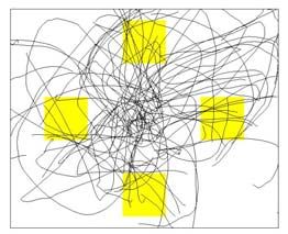
5

recording, subjects viewed a computer monitor that displayed task information related to various
cursor control tasks as described below.
  We refer to each session with the notation: -; for example S3-
40 is the session for participant S3 on day 40 after implantation.    Sessions analyzed in the present
study fell into one of three categories based on the type of training task and the decoding algorithm,
referred to as . PLP sessions tested Position decoding
using a Linear filter trained with a Pursuit tracking task; VKC sessions tested Velocity decoding
using a Kalman filter trained with the Center out task; and VLKC sessions tested Velocity decoding
using Linear and Kalman filters trained on the same day with the Center out task. The various tasks
are described in detail below. The analyses here are based on all complete sessions between 40 and
418 days after implant in S3 and 85 to 224 days after implant in A1 for which the decoding and
cursor control evaluation methods studied here were used.

  Table 1. Categorization of the recording sessions based on decoding algorithms and training task.
   Session group label:
                                    Session index                Decoding
     kinematic model,                                                               Training task
                                     (unit count)                algorithm
  decoding method, task
                              S3-40 (179), S3-48 (159),
Position, Linear filter,                                    Position-based        Random pursuit-
                              S3-54 (147); A1-85 (103),
pursuit tracking (PLP)                                      linear filter         tracking task
                              A1-91 (117)
                              S3-254 (46), S3-261 (80),
                              S3-280 (13), S3-282 (20),
Velocity, Kalman filter,                                    Velocity-based        Center-out-back
                              S3-285 (15), S3-287 (33),
Center out (VKC)                                            Kalman filter         task
                              A1-197 (102), A1-216
                              (70), A1-224 (85)
                                                            Velocity-based
Velocity, Linear/Kalman,      S3-408 (25), S3-412 (28),                           Center-out-back
                                                            linear and Kalman
Center out (VLKC)             S3-418 (21)                                         task
                                                            filters

2.3. Training

2.3.1. Training procedure. A main purpose of “training” in our clinical study was to set the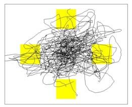
6

parameters of the decoding algorithms such that they define an optimal mapping between neural
activity and cursor control signals. A training procedure was developed previously (see Hochberg et
al. [13]) to simultaneously obtain neural activity patterns and cursor kinematics to enable the
estimation of the decoding algorithm parameters without accompanying limb movements. In this
procedure, a training cursor (TC) was displayed on a computer monitor and moved to generate
cursor trajectories (details below).   During this presentation, the participants were instructed to
imagine moving their arm or hand as if they were controlling the TC.        Neural signals recorded
during this imagined movement together with the TC kinematics (position or velocity) were used to
train the decoding algorithms.
  The overall training procedure was composed of a series of short recording periods, called
“blocks,” each of which lasted 1-1.5 min. We devised two types of training blocks: open-loop (OL)
and closed-loop (CL) blocks. In OL blocks, the TC and the target were shown together on the
monitor. The number of OL blocks varied over session groups: four 1-min OL blocks for PLP
sessions, two (mean 2, s.d. ±1) 1.2-min blocks for VKC sessions and three 1.5-min blocks for
VLKC sessions. We used the data from the OL blocks to train an initial decoding algorithm.
  The OL blocks were followed by several closed-loop (CL) blocks in which a feedback cursor
(FC) was simultaneously displayed on the monitor with the TC.       The FC motion was determined
using the decoding algorithm trained from the OL trials.      The presentation of the FC provided
additional information through visual feedback to the subjects about how well their intended actions
were being decoded. FC presentation was motivated by an assumption that the participants might
adjust their neural activity to improve cursor control by seeing the error between the FC and TC.
The decoding algorithm was re-trained at the end of every other CL block to incrementally update
the parameters. Four 1-min CL blocks were used in PLP sessions, six (mean 6, s.d. ±2) 1.2-min
blocks in VKC sessions and four 1.5-min blocks in VLKC sessions. See Figure 1a for an illustration
of the procedure of OL and CL training.
  In PLP recording sessions, the TC was moved manually by the technician. In VKC and VLKC
sessions, the TC was moved by a computer-generated bell-shaped velocity profile (Figure 1b) to
provide the participants with well-defined velocity training patterns. The participants rested
between blocks for a short period (~ 1 min on average).
2.3.2. Cursor movement tasks for training decoding algorithms. Two different training tasks were
used depending on the representation of cursor kinematics (position or velocity): position-based
decoders were trained using a random target pursuit-tracking task [13-14] while velocity-based
7

decoders were trained using a center-out-and-back (to center) task [32-33]. Note that during training
a TC was always present on the screen. This made these training tasks more similar to pursuit
tracking than step tracking. However, during testing, only the NC was present under closed loop
control and the tasks can be seen as step-tracking tasks.
  In the random pursuit-tracking task, the TC moved from a starting location towards a target that
was randomly placed on the screen. When the TC intersected the target, an audio feedback cue was
provided and the next target immediately appeared at another random location, keeping only one
target at a time on the monitor. This task had the important property of spanning much of the space
of screen positions, which provided the decoder learning method with a wide range of cursor
position samples (see Figure 1c for example of TC positions). The target and the TC occupied
90×90 pixels (visual angle: 3.8º) and 60×60 pixels (2.5º) of the screen, respectively, where the total
screen size was 800×600 pixels (17” monitor). The distance from the participants’ eyes to the center
of the monitor was approximately 59cm and the visual angle of the workspace on the screen was
approximately 34.08º. The size of the FC during CL blocks occupied 102×126 pixels (4.3º×5.3º).
  In the center-out-back task, four peripheral targets (0º, 90º, 180º and 270º) and one center target
were displayed on the screen. The TC started at the center target, holding there for 1.2s, and then
began moving to one of four peripheral targets which was highlighted. When the TC reached the
target it remained there for 0.5s before tracing its path back to the center target. The point-to-point
TC movement followed a bell-shaped computer-generated speed profile (Figure 1b) that spanned T
seconds. The reaching time, T, varied across the session in the range [1.5s, 4.5s]. A single center-
out-back TC trial took (1.7 + 2T) seconds. The target location was pseudo-randomly selected by a
predetermined program. We used the center-out-back task instead of the standard center-out task
with re-centering. In this latter task, a cursor moves smoothly from the center to peripheral targets
but then jumps automatically back to the center target. This procedure causes cursor position and
velocity to be highly correlated with each other. In contrast, the center-out-back task enables us to
sample two opposite cursor velocities for each cursor position. This makes it easier to uncover
whether a modulated neural activity is related to position and/or velocity. In the earlier sessions
including S3-{254, 261, 280, 282} and A1-{197, 216}, the target, the TC and the FC occupied
90×90 (3.8º), 60×60 (2.5º) and 60×60 (2.5º) pixels, respectively. The distance from the center to the
target was 210 pixels (8.9º). In the later sessions including S3-{285, 287, 408, 412, 418} and A1-
224, the sizes of the target, the TC and the FC were reduced to 48×48 (2.0º), 40×40 (1.3º) and
40×40 (1.3º) pixels, respectively. The distance from center was increased to 255 pixels (10.8º) for
vertical targets and 300 (12.7º) for horizontal targets to more completely cover the screen space.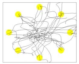
8

2.4. Neural cursor control testing tasks
A closed-loop center-out-back task was used to evaluate neural cursor control performance. This
testing task shared a basic structure with the center-out-back training task, however differed in
several respects (see below). The NC was not automatically re-centered, making this task closer to
normal continuous computer mouse activities than the standard, re-centering, center-out task [34].
  The center-out-back testing task used in PLP and VKC sessions was the same as the one used in
Hochberg et al. [13]. A target (120×120 pixels; visual angle: 5.1º) was positioned at one of four
fixed locations (0°, 90°, 180°, 270°) with the distance of 210 pixels (8.9º) from the center and the
participant was asked to control the NC (60x60 pixels; 2.5°) to acquire the target. If the NC reached
the target and dwelled on it longer than a preset period (500ms), the target was deemed to be
acquired and audio and visual feedback was given for 1s. If a timeout period (7s) elapsed before
target acquisition, another audio feedback cue was provided indicating failed target acquisition
(with no change of the target icon). After target acquisition or failure due to timeout, the target was
relocated to the screen center and the participant had to move the NC to acquire it before starting
the next target acquisition trial. There was no time limit for this center target acquisition. Data
collected during center-target acquisition is not analyzed in this study.
  In VLKC sessions, a more challenging center-out-back testing task was used. There were eight
peripheral targets and one center target presented on the screen. Smaller targets were located further
from the center: the sizes of the targets and the NC were 48×48 (2.0º) and 40×40 (1.7º) pixels,
respectively, and the distances from center to the targets were 255 pixels (10.8º) for vertical
direction and 300 (12.7º) for horizontal direction, respectively. A trial could end without success not
only when the timeout period was exceeded but also when a false target was acquired. The timeout
period was 10s for this task. Compared to the above four-target testing task, this task increased the
index of task difficulty (ID) [27] by 2.5 times, increased the number of targets, and added another
failure condition by allowing the potential selection of false targets.
9
(a)
OL training block CL training block Testing blocks
... ...
time
Training cursor Feedback cursor Neural cursor Target
(b) (c)
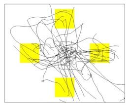
Figure 1. Training paradigm. (a) Illustrations of a series of open-loop (OL) training (left), closed-loop (CL)
training (middle) and testing blocks (right). In the OL block (1-1.5 min period of recording), the training
cursor (TC) was moved by a technician or a computer program to reach a target. After one to four OL blocks,
CL training blocks included a feedback cursor (FC), controlled by decoded neural signals in real time, that
was also displayed on the monitor to provide visual feedback to the participants. In testing blocks, the
participants volitionally controlled a neural cursor (NC) to reach and dwell (for 500ms) on targets. (b) An
example of the computer-generated speed profile for the TC. Here, a speed value of 0.1/sec represents moving
10% of the screen height per second. Across all the sessions included in this study, the speed profile duration
varied from 1.5s to 4.5s. (c) An example of the TC positions collected for 8 min during the random pursuit-
tracking task used for training the position-based decoding algorithm (from the session S3-40). The screen
space was normalized to [-0.6 0.6] in the horizontal axis (denoted X here) and [-0.5 0.5] in the vertical axis
(Y).
2.5. Decoding algorithms
Decoding is the process of converting recorded neural signals (e.g. firing rates) into cursor
movement. In this study, we compared two decoding algorithms: linear filtering versus Kalman
10

filtering.
  Let xt be a D×1 vector of cursor kinematics such as position [px, py]T or velocity [vx, vy]T in the x
(horizontal) or y (vertical) direction sampled at a discrete time instant t. D = 2 in this study as we
decode the 2D cursor kinematics, yet the decoding algorithms presented here can be extended for
the cases with D > 2. Note that decoding velocity (i.e. xt = [vx vy]T) is equivalent to decoding
direction and speed in the polar space. Let zt be an N×1 vector of firing rates of N units observed at t.
Firing rates for each unit were approximated using spike counts computed in fixed, non-overlapping,
time bins. The bin size was set as either 50ms for PLP sessions or 100ms for the remainder of the
sessions. Decoding algorithms establish a causal relationship between these neural firing rates and
the cursor kinematics such as position or velocity.

2.5.1. Linear Filter. Using the linear filter, each dimension d of the current kinematic vector xt was
predicted separately using a linear combination of the current and past firing rates, zt, zt-1, …, zt-L+1:
                                                   L −1
                                 x td = bd + ∑ w Ti ,d z t −i + ε t , for d = 1,…, D,                                  (1)
                                                    i =0

where L denotes the length of the firing history, εt is a random variable assumed to be white
Gaussian noise with zero mean, bd is a scalar bias term for dimension d and wi,d is an N×1 vector of
filter coefficients for dimension d and zt-i. Motivated by previous intracortical brain-computer
interface (BCI) studies that took L to be approximately a one-second history of firing rates [1-4],
here L was chosen to be 20 (bins) when 50-ms bins were used or 10 (bins) when 100-ms bins were
used. The optimal linear weights ŵd = [ŵ0,dT,…, ŵL-1,dT]T were obtained using least squares
regression to minimize the mean squared error between estimated and training cursor kinematics.

2.5.2. Kalman Filter. The Kalman filter [35] is a Bayesian inference algorithm that recursively
infers the cursor kinematics from the history of firing rates. In this formulation, inference of
kinematic signals xt conditioned on the whole observation of firing rates with a possible time offset
j, z1:t-j = {z1, z2, …, zt-j}, is performed through recursive Bayesian estimation [25]:
                                            1
                    p(x t | z 1:t − j ) =       p(z t − j | x t ) ∫ p(x t | x t −1 ) p(x t −1 | z 1:t −1− j )dx t −1   (2)
                                            κ
where κ is a normalization constant. In this estimation, the a posteriori probability p(xt | z1:t-j) at
time t is inferred by updating the previous estimate p(xt-1 | z1:t-1-j) at t-1 using a system model p(xt |
xt-1) and an observation model p(zt-j | xt) with neural data zt-j. The observation model describes how
the observed firing rates at t-j (with a possibly non-zero lag offset j) are generated from kinematics
11
xt and the system model describes how the cursor kinematics evolve from t-1 to t. In the Kalman
filtering algorithm, the observation model and the system model are approximated as linear
Gaussian models
z t − j = Hx t + q t , q t ~ G (0, Q)
(3)
x t = Ax t −1 + ω t , ω t ~ G (0, Ω)
where H and A are time-invariant linear coefficient matrices for each model and qt and ωt are
random vectors distributed with zero mean Gaussian noise with covariance matrices Q and Ω,
respectively. G(·) here denotes a multi-variate Gaussian distribution. Note that zt and xt are centered
to be zero mean vectors. The parameters H, A, Q and Ω are estimated from training data using a
least squares method. Given the learned model, decoded kinematics can be inferred at every time
instance using a closed-form recursion. Details of the model training and use of the Kalman filter
for neural decoding can be found in Wu et al. [24-25].
It is worth noting that both the linear filter and the Kalman filter integrate the neural signals over
time. The linear filter achieves this by explicitly building a finite impulse response (FIR) filter with
a 1s memory of the firing rate history where the FIR filter tends to pass the low frequency signal.
The Kalman filter does this by the recursive equations, integrating the information from the history
of neural signals (see [25] for comparison between two filters). A fundamental difference between
the filters is that the Kalman filter is a Bayesian model that, in addition to modeling the relationship
between the neural and movement signals, also incorporates a prior model of the cursor movement.
2.6. Correlation analysis during open-loop training
To evaluate the relationship between the firing rates and the TC kinematic parameters independent
of a specific decoding method, we computed the Pearson correlation coefficient (CC) [36] between
the firing rate for each unit and the TC kinematic parameters during the OL training blocks
collected from multiple sessions where either the random pursuit-tracking or the center-out-back
task was used. In our analysis, each unit’s firing rate was smoothed by a low-pass filter with a unit
gain and a cutoff frequency at 0.2*fs. Here, fs represents a sampling frequency for the firing rate and
is set to 10Hz (corresponding to the 100ms bin width). To account for latency between the TC
movement and motor cortical activity, we computed the CC for each unit at time lags from j = 0s,
0.1s, …2s where the lag j means the firing rate leads the kinematic signals by j seconds. We
empirically searched for the optimal lag at which the CC was maximized. Note that we only
explored non-negative lags to maintain a causal relationship between firing and movement. This is
necessary as neural activity must precede action for effective closed-loop cursor control.12
Specifically, let zit-j be the smoothed firing rate of unit i at the time instant t-j and xdt be the dth
dimension of the kinematic parameter vector xt. The CC between zit-j and xdt was estimated from
data using:
E [( z ti− j − z i )( xtd − x d )]
CC (i, d ) = , (4)
s z sd
where z and sz (respectively, x and sd) are the mean and standard deviation of zit-j (or xdt ), and
E[·] represents the expectation. Further, we used the absolute value such that |CC(i,d)| = 0 represents
no correlation and |CC(i,d)| = 1 corresponds to perfect correlation (including perfect inverse
correlation). The significance of the correlation for each unit was evaluated using a t-test (with
significance determined at the 1% level). If a unit showed significant correlation with this test for
the at least one dimension of xt at any lag j, then the unit was considered to be significantly
correlated with xt.
2.7. Decoding accuracy during closed-loop training
To evaluate cursor decoding performance during CL training blocks we computed the CC between
the TC and the FC kinematics in each block. Since the number of CL blocks varied across sessions,
we evaluated only the first four CL blocks collected from each session. After finding an optimal lag
as above, the CCs for each of the vertical and horizontal kinematic parameters were averaged. We
used Fisher’s transform [37] to estimate a 95% confidence interval for the CC estimated in each
block.
2.8. Evolution of directional tuning
Velocity-based decoding specifically exploits the directional tuning of motor cortical units that
persists in humans with tetraplegia [13, 26]. To investigate the consistency of this directional tuning
we analyzed whether the directional tuning of individual units changed between training and testing
epochs. This analysis was applied to the recording sessions where velocity-based decoding was
performed (6 sessions for S3 and 3 sessions for A1). In this analysis, we used a cosine tuning
function [17] to fit the firing rates as a function of cursor direction. This approach has been widely
used for studying neural tuning to arm/hand direction in non-human primates. For training epochs,
we computed the tuning function using the TC direction. For testing epochs, where the TC was not
present, we computed the tuning function with the intended direction that was defined as a direction
from the current position of the NC to the designated target (see [26] for introduction of the
intended direction). Using the cosine tuning function fit to the firing rates of individual units, we13
computed the preferred direction (PD) and the tuning depth (TD) for each unit. The PD is a
direction at which the fitted firing rate is maximal and the TD is the difference between the
maximum and minimum values of the fitted firing rate. The confidence intervals of the estimated
PD and TD were obtained with a bootstrap algorithm (bias corrected percentile method, 103
bootstrap re-samples) [38]. The PD (or TD) of each unit was considered to have changed
significantly between training and testing epochs if the 95% confidence interval of the PD (or TD)
estimated during testing did not overlap the 95% interval estimated during training.
2.9. Performance evaluation measures
To quantify NC control performance, we applied performance measures used in the field of human
computer interaction (HCI) to evaluate pointing devices. The measures are composed of two
categories, including gross measures that evaluate the overall performance of a given task as
defined in the ISO9241-9 standard [27], and more detailed measures that evaluate the spatio-
temporal properties of continuous point-to-point movements [28].
Of the gross measures, we evaluated speed and accuracy of cursor control by computing mean
movement time (MT) and error rate (ER) in target acquisition. MT was measured as the average
time it took to reach and dwell on the target from a starting point. Here we measured MT for the
trials only when the target was acquired. ER was defined as a percentage of the trials in which a
designated target was not acquired. Note that in this study we do not report an information-theoretic
throughput measure standardized by ISO9241-9 since it requires tasks with a range of task
difficulties not present in our tests.
We also computed four fine performance measures adopted from MacKenzie et al. [28],
including orthogonal direction change (ODC), movement direction change (MDC), movement error
(ME) and movement variability (MV); these are illustrated in Figure 2. Given a task axis defined as
a straight line connecting the starting position to the target position, ODC measures how
consistently the cursor moves towards a target by counting direction changes orthogonal to the task
axis and MDC measures the straightness of the NC path by counting direction changes parallel to
the task axis. ME measures how much the NC path deviates from the ideal straight line (i.e. task
axis) by computing the average deviation of NC positions from the task axis:
1 m
ME = ∑ yi (5)
m i =1
where yi is a distance (positive or negative, see Figure 2) from the i-th sample point on the NC path
to the task axis and m is the number of the NC samples from the starting point to the target. MV14
measures the variability of the NC path by computing the standard deviation of yi:
m
2
∑ ( yi − y )
i =1
MV = . (6)
m −1
(a) MDC (b) ODC
start target
task axis
(c) Large ME, Large MV (d) Large ME, Small MV
yi
Figure 2. Illustration of the NC path performance measures. (a) MDC counts the number of movement
direction changes parallel to the task axis (for instance, MDC = 2 in this example). (b) ODC counts the
number of direction change orthogonal to the task axis (ODC = 2). (c-d) ME measures movement deviation
by computing the average of the absolute deviations |yi| from the task axis, and MV measures the standard
deviation of yi. Two cases are illustrated in which both ME and MV are large (c) or ME is large but MV is
small (d). (Illustration derived from MacKenzie et al. [28].)
2.10. Chance performance
We further evaluated neural cursor control performance in terms of decoding accuracy and target
acquisition rates relative to chance as described below. These evaluations use estimates of chance
performance and are dependent upon details of the task configuration and the decoding algorithm.
Here we present methods of estimating two different chance performance measures: chance
decoding accuracy during training and chance target acquisition rate during testing.
The chance decoding accuracy during training was estimated by training and testing a decoder
with shuffled data in which neural signals and the TC kinematics were shuffled to be uncorrelated.
To create surrogate data, we first randomly selected K (> 2) training (OL or CL) blocks from a15 single recording session. Then, we replaced the TC data of the first K-1 blocks with different TC data that were randomly selected from different recording sessions in which the same training task was used. A decoder was trained using the data in these K-1 blocks. The trained decoder was then used to decode the TC kinematics from neural signals for the Kth block. The CC between the estimated and the true TC kinematics in this testing block was measured. This procedure was repeated 103 times to obtain an average chance level for the CC. We estimated the chance level for each pair of the decoder and the associated training task (i.e. the position-based linear filter with random pursuit-tracking or the velocity-based Kalman filter with center-out-back). We also estimated chance performance for the closed-loop center-out-back target acquisition task (4 or 8 peripheral targets). In an off-line analysis we characterized the chance target acquisition rate by estimating the probability that the target would have been acquired by accident if the participant were not aware of the actual target location but only knew that it should be one of four (or eight) possible target locations. Again, target selection was determined by whether the NC dwelled on a specific target for 500ms or more. If the NC were perfectly controlled, the baseline chance rate would be 25% for four targets (12.5% for eight). Depending on the characteristics of the NC decoding method, however, this baseline chance rate may not reflect the “true” rate of selecting a target by accident. If neural control produced straight but not perfect trajectories, the chance rate would likely be lower by an amount proportional to the target acquisition performance; for instance, if NC control with some decoding algorithm resulted in acquisition of 80% targets, the baseline chance rate would be adjusted to 20%. If, instead, the decoding algorithm yielded “unsteady” NC movements that could span a wide range of the computer screen, the NC could intersect and dwell on any of the target locations accidently. This could increase the chance rate for a particular decoder above the baseline; this rate can be computed by simulation. Any decoder- specific changes to the baseline chance rate result in what we call the adjusted chance rate. In this case, the difference likely reflects the effect of unsteady NC behavior on target acquisition performance. Below “chance rate” is used to mean the adjusted chance rate. In this post-hoc analysis, we ran a computer simulation using the data recorded during performance of the target acquisition task. For each “simulated” trial, we used a true NC trajectory with a randomly placed target at one of four or eight possible locations; in this way we decoupled the observed NC trajectory from the original goal. The chance rate was computed as the percentage of the trials when the NC moved to the random target and dwelled on it for 500ms within the timeout period. For each decoder, we repeated this procedure 103 times to obtain the average chance rate. The simulated data were collected from specific session datasets for different decoders (see
16

Table 1): five PLP sessions for the position-based linear filter with 4 targets (total 400 target
acquisition trials); nine VKC sessions for the velocity-based Kalman filter with 4 targets (521
trials); and three VLKC sessions for the velocity-based linear and Kalman filters with 8 targets (90
trials with the linear filter and 102 with the Kalman filter, respectively).
  The method defined above results in a chance rate that is generally higher than that used in
Hochberg et al. [13].   For consistency and comparison with that earlier study we also measured the
control chance rate (control rate) for the 4-target tasks (see [13] for details).     In this off-line
analysis, both the correct target and a single false target (randomly selected from the three other
targets) were placed on screen during each post-hoc trial. We measured the percentage of the trials
in which the NC passed through (and dwelled on) the false target by accident before it reached the
correct target. Note that we did not have to perform this off-line analysis for VLKC sessions since,
for these sessions, all eight targets were shown simultaneously and a false target could be selected
on-line if the NC dwelled on it; thus, this is already included in the error rate.
  Finally, we define a significant target acquisition rate (STAR) as the difference between the
observed target acquisition rate and the control rate. This STAR quantifies what portion of the
observed target acquisition rate is indeed achieved by intentionally moving the NC to the target.
STAR is useful to compare cursor control performance when the control rate varies across different
decoders on identical tasks.

3. RESULTS
We investigated the impact of several NIS design choices on neural cursor control by two
participants with tetraplegia (S3 and A1). Both participants obtained neural control of a computer
cursor during the performance of a four-direction radial target acquisition task and results are
reported for 17 sessions ranging from 40 to 418 days after implantation of the array in which the
center-out-back task was used to assess the performance (with variations as described in Methods).
Neural activity was observed in all these sessions and the number of spiking units detected per
session varied from 13 to 179 (mean 63.8, SD 61.9, 12 sessions) for S3 and from 85 to 117 (mean
95.4, SD 18.2, 5 sessions) for A1, respectively. The units were isolated by utilizing signal
processing and spike sorting methods applied previously in this ongoing trial [13].
  In several experiments below we explored five important issues relevant to developing an NIS: 1)
Tuning of neuronal units to cursor position and velocity during OL training; 2) The effects of OL
and CL training on acquisition of cursor control with position or velocity; 3) The stability of
directional tuning between training and testing; 4) The closed-loop performance of position-based
17

cursor decoding using the linear filter versus velocity-based decoding using the Kalman filter; 5)
The importance of the kinematic representation versus the decoding algorithm for cursor control.

3.1. Kinematic correlation analysis
The CC between the firing rate and the kinematic parameters was measured for every unit recorded
during the OL training blocks where the participants imagined arm/hand movements following the
TC motion. During OL training neural activity should be related to the properties of any imagined
movement (or, perhaps, the observed visual stimulus) and is independent of any particular decoding
algorithm since no NC is presented. The analysis was performed with 1226 units recorded in both
participants recorded over 17 recording sessions.
      We first computed the optimal lag for each unit at which the CC was maximized. The
distribution of the optimal lag over the neural population is shown in Figure 3a and reveals that for
most units the CC was maximized at zero lag for both position and velocity. Based on this analysis
we assume zero lag for all the Kalman filter decoders used in this study (namely, j = 0 in equation
2).
  From the statistics of the CC measures, we found that the firing rates of the majority of units in
both participants were more strongly correlated with cursor velocity than with position (Figure 3b-
d). The statistical test (see Methods 2.6) showed that 65.3% of units were significantly correlated (t-
test; p < 0.01) with both position and velocity, 5.7% with position alone and 24.7% with velocity
alone. This result indicated that 95.7% of all the units detected by the microelectrode array in
human motor cortex were significantly correlated with at least one of the TC kinematic parameters.
The CC values for velocity were overall larger than those for position (p
18 (a) (b) (c) (d)
19

Figure 3. Analysis of kinematic tuning during training. (a) Histograms showing the percentage of units
with optimal lags ranging from 0 to 2s (1126 neuronal units from 17 recording sessions in two participants
(S3 and A1)). (b) The correlation coefficients (CC) between individual firing rates and kinematic parameters –
position (white) vs. velocity (gray) - during open-loop training blocks. The median of the CC values is
represented by bars and 25% and 75% percentiles by vertical lines. (c) The percentage of units significantly
correlated (Methods) with either position or velocity (p < 0.01; t-test). The number of units (N) recorded in
each session is denoted in parentheses. (d) The percentage of units that showed stronger (and significant)
correlation with one of position or velocity compared to the other.

3.2. Effect of training procedures on cursor control
We evaluated how cursor control was achieved through the training procedures presented in this
study for different decoding algorithms. Two decoding algorithms were considered here including
the position-based linear filter trained with the random pursuit-tracking task and the velocity-based
Kalman filter trained with the center-out-back task. In particular, we studied how much OL training
alone enabled cursor control for each decoding algorithm and how much CL training improved that
performance. To quantify this, we computed the CC between the TC and the feedback cursor (FC)
kinematic parameter (position or velocity depending on the algorithm used). We obtained the
average CC (averaged over the horizontal and vertical axes at the optimal lag for each block, see
Methods) for each of the first 4 CL blocks from 14 recording sessions (PLP and VKC) in both S3
and A1. The optimal lag averaged over 14 sessions at which the CC was maximized was 0.47s (s.d.
0.4s) which means that the TC led the FC by 0.47s.
  Figure 4 shows the comparison of the CC for the two decoding algorithms. In both participants
the CC obtained with the position-based linear filter registered a much lower value in the first CL
block and improved considerably during the remaining blocks. On the other hand, the CC obtained
with the velocity-based Kalman filter reached over 0.5 in the first CL block and improved only
slightly afterwards. Note that, in addition to having higher CC’s, the velocity-based decoding results
in S3 were all obtained with fewer units than the position-based results (see Table 1). In our
experiments, an average of 2.4-min of data (2 OL blocks) were required to train the velocity-based
Kalman filter to achieve the CC > 0.5 and 8-min of data (4 OL + 4 CL blocks) were required to train
the position-based linear filter to achieve similar accuracy.
  This result suggests that training the velocity-based Kalman filter with the (4-target) center-out-
back task required less training time compared to training the position-based linear filter with the
random pursuit-tracking task. We did not investigate whether such rapid training was made possible
20

due to decoding velocity, which was more correlated with neural activity (Section 3.1), or using a
relatively simpler center-out task, or both.           For practical NIS development however, we can
conclude that less training time is required using the velocity-based Kalman filter with the center-
out-back task.

 (a)                                                    (b)

               position-based linear filter decoding          velocity-based Kalman filter decoding

Figure 4. Decoding performance improvement with training. Evolution of the average CC between the TC
and the FC trajectories of position or velocity during closed-loop (CL) training blocks for S3 (a) and A1 (b).
CC = 1 represents perfect correlation between the TC and the FC. The CC was measured for the two groups
of CL blocks separated based on the decoding method used: the position-based linear filter (white) and the
velocity-based Kalman filter (gray). The bars to the left side of a vertical dashed line illustrate the chance
level for decoding accuracy (Methods) for each decoding method. The bars and the vertical lines to the right
side represent the average CC and the 95% confidence interval during each of the 1st to the 4th CL blocks.

3.3. Evaluation of changes in directional tuning from training to testing
Previous animal studies have sometimes shown significant changes in directional tuning of cells
between open-loop and closed-loop neural control [4-5]. Consequently we sought to establish
whether the directional tuning of cells was stable or changed between training and testing in
tetraplegic humans using an NIS over a series of training and testing periods (total 30-60 min).
Since here we focused on directional tuning change we analyze data from VKC sessions that
explicitly decoded velocity (207 units in S3 from six sessions: S3-{254, 261, 280, 285, 286 and
288} and 257 units in A1 from three sessions: A1-{197, 216 and 224}). A statistical analysis of
21 tuning change revealed one class of units that was consistent and another class that changed over time. Figure 5 illustrates three example units that were consistently tuned to the TC direction across training and testing (recorded from S3-261). From the last two CL training blocks of S3-261, we sampled the spike trains of three units within a 1s time window from the onset of the target appearance in one of four directions (0º, 90º, 180º, 270º). Nine spike trains per unit, per direction are shown in the left column of Figure 5. The arrows in the circle represent the estimated preferred direction (PD) of each unit. The right column of Figure 5 shows the directional tuning of these units during testing where the four-target center-out-back task was performed. Since the NC could move to any point on the 2D task space (i.e. computer screen), the intended direction was continuously distributed from 0º to 360º. Therefore, we divided the space of the intended direction into eight equally spaced angular bins centered at (0º, 45º, 90º, 135º, 180º, 225º, 270º, 315º). Nine 1s spike trains for each angular bin are presented here. Visual comparison of the spike raster plots between the left and the right columns of Figure 5 suggests that directional tuning of these units did not change substantially from training to testing. This also illustrates that even when trained using only four directional movements, spiking activities of these units were broadly tuned over a wider range of directions, thus enabling the NC to move in any direction after training. In contrast, Figure 6 illustrates two examples of the units (from A1-197) that changed their directional tuning between the training (left) and testing (right) periods. These units showed statistically significant changes in the PD from training to testing, although the tuning depth of these units in A1 (Figure 6) was not as large as those in S3 (Figure 5). We remark here that these results do not conclusively demonstrate that human motor cortical neurons exhibit rapid PD changes. Rather, Figures 5 and 6 show examples of the neuronal units that sustained or changed their preferred directions within a 2 h recording period. We preformed a statistical analysis of the tuning change for all 464 units (207 units in S3 and 257 in A1) to find how many units changed or sustained directional tuning and how much their preferred directions and tuning depths were changed. First, the percentage of units that were significantly tuned to direction (F-test, p < 0.01) increased from 69.6% (144 units) during training to 80.2% (166 units) during testing in S3 and from 35.0% (90 units) to 63.4% (163 units) in A1. Of those units that had been tuned during training (144 units in S3 and 90 in A1), 4.9% (7 units) in S3 and 24.4% (22 units) in A1 lost directional tuning during testing. Of those units that were not tuned during training (63 units in S3 and 167 units in A1), 46.0% (29 units) in S3 and 56.9% in A1 (95 units) gained directional tuning during testing. Of those units that were tuned during training, 95.1% (137 units)
22

in S3 and 75.6% in A1 (68 units) remained directionally tuned from training to testing.
  Second, among those units that remained directionally tuned from training to testing, we
evaluated how much their PD changed. Note that the PD was deemed to be significantly changed if
the two 95% confidence intervals computed in training and testing respectively did not overlap (see
Methods 2.8). We found that 72.9% (100 out of 137 units) in S3 and 42.7% (29 out of 68 units) in
A1 showed no significant change in PD (95% confidence). For the other units in which the PD
significantly changed, the average change in angle was 34.1º (s.d. 20.4º) for S3 and 99.7º (s.d.
56.6º) for A1, respectively. Figure 7 summarizes these results.
  Finally, we evaluated the change of the tuning depth of those units that remained directionally
tuned (137 units in S3 and 68 in A1) between training and testing. We found that 24.8% (34 units)
in S3 and 33.8% (23 units) in A1 changed their tuning depths significantly (95% confidence).
Among these units, 82.4% (28 units) in S3 and 82.6% (19 units) in A1 increased the tuning depth
and 17.6% (6 units) in S3 and 17.4% (4 units) in A1 decreased the tuning depth. On average, the
tuning depth increased by 61.9% (s.d. 68.2%) from training to testing (over 34 units) in S3 and by
130.8% (s.d. 122.1%, over 23 units) in A1, respectively; this increase in the tuning depth was
statistically significant (paired t-test, p ≈ 7.8 × 10⁻⁶ for S3 and p ≈ 3.8 × 10⁻⁵ for A1). The increases
in the tuning depth and in the number of tuned units during testing suggests that directional tuning
in MI firing activity became stronger between training, where the participants imagined following
the visually guided cursor movements, to testing, where they volitionally moved the cursor.
   Although we did not perform an extended study of the relationship between consistency in
tuning and cursor control performance, we posit that the larger number of tuning changes in the
neuronal population of A1 might partially explain A1’s poorer cursor control performance relative
to S3 (see the following section).
23

(a) Channel 1, unit 1
                    Training   Testing

(b) Channel 33, unit 1

(c) Channel 86, unit 2
24
Figure 5. Consistent directional tuning between training and testing. Sample spike trains are shown for
three example units in one session (S3-261), in which S3 performed the center-out-back task during training
(left) and testing (right). Black tics in the raster plots show the times when neuronal spikes occurred after
target onset. Spike raster plots are arrayed according to the direction of movement (4 directions during
training and 8 during testing). The arrows indicate the preferred directions estimated for each unit. The bars
below the spike raster plots show the histogram of spikes for 1s in 100ms non-overlapping windows.
(a) Channel 82, unit 1, A1-197
Training Testing
(b) Channel 27, unit 1, A1-224
Figure 6. Changes in directional tuning between training and testing. The spike trains of two sample
units from A1-197 (a) and A1-224 (b) are shown. The left and right columns illustrate tuning during training
and testing, respectively. The arrows indicate the estimated preferred direction (PD).25
(a) Tuning statistics of neural population (b) Degree of change in PD for those units
whose PD changed
S3
Not tuned Tuned (training) Tuned (testing)
Always tuned PD unchanged PD changed
A1
Figure 7. Statistics of directional tuning change. (a) The statistics of tuning across training and testing is
illustrated in terms of the percentage of subsets of units with particular properties in S3 (over 6 sessions) and
in A1 (over 3 sessions). The neural population was divided into four subsets including: units showing no
directional tuning across the session, units directionally tuned only during training, units tuned only during
testing, and units tuned during both training and testing. The last subset is further divided into smaller groups
including: one showing significant PD changes and the other showing no PD change. (b) For units that
changed PD, the bars indicate the percentage of units that changed by the indicated number of degrees (0-30,
30-60, etc.) for S3 (blue) and A1 (red).
3.4 The velocity-based Kalman filter versus the position-based linear filter
Based on the tuning analysis above we compared on-line cursor control in tetraplegic humans using
the velocity-based Kalman filter with the position-based linear filter adopted from Hochberg et al.
[13]. We found that cursor control performance was significantly improved with the velocity-
based Kalman filter for both participants. We evaluated performance in the four-target acquisition
task across those recording sessions in which the identical task configuration was used (9 sessions
for S3, 5 for A1). The number of target acquisition assessment trials was 80 per session except S3-
285 (44 trials), S3-287 (73), A1-197 (30), A1-216 (12) and A1-224 (43). In each trial, the
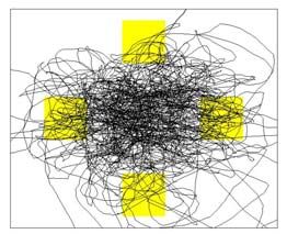
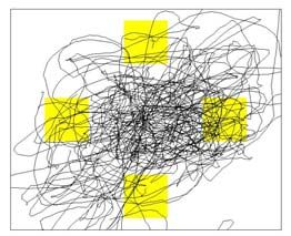
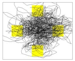
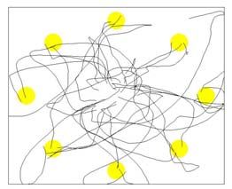
participants had to acquire the target before a 7s timeout.26 Figures 8-11 illustrate the performance of the two decoding methods. The figures present the decoded NC paths starting from the center and moving to each of four peripheral targets for all 14 recording sessions, along with the mean NC paths. These figures show that the NC paths decoded with the velocity-based Kalman filter were much straighter and smoother than those produced by the position-based linear filter in both participants. Note that the NC movements using the velocity- based Kalman filter were achieved with fewer units: the ratios of the average unit counts for the position-based linear filter sessions compared with the later velocity-based Kalman filter sessions were 162:35 for S3 and 110:86 for A1. Using pointing device performance measures based on the ISO 9241-9 standard as well as other cursor control measures (see Methods), we quantified the performance of closed-loop neural cursor control for each participant, as summarized in Table 2. The control chance rate was 9.8% for the position-based linear filter, which was on a par with previously reported results in a different participant [13]. For the velocity-based Kalman filter, the control rate was 3.9%. This lower control rate suggests that the better controlled NC trajectories produced by the velocity-based Kalman filter reduced the chance of selecting an incorrect target; this is a significant advantage in a real task where many targets are simultaneously placed and false targets could be selected (see Methods for the estimation of the control rate). For S3, target acquisition accuracy improved using the velocity-based Kalman filter over using the position-based linear filter. S3 failed to acquire 52 out of 240 targets before the timeout (ER = 21.7%) using the position-based linear filter over 3 sessions versus 60 out of 436 targets (ER = 13.8%) using the velocity-based Kalman filter over 6 sessions, reducing the absolute value of ER by 7.9%. For the observed target acquisition rate (78.3%) using the position-based linear filter, the baseline chance rate for the 4-target center-out task was 19.6% (i.e. a quarter of the target acquisition rate). However, the adjusted chance rate obtained from simulation was 25.9%, higher than the baseline chance rate by 6.3%. This implies that there was a 6.3% chance that an incorrect target was selected by accident due to unsteady NC behavior. The baseline chance rate for the velocity-based Kalman filter (target acquisition rate = 86.2%) was 21.6%. The adjusted chance rate was 23.9%, 2.3% higher than the baseline chance rate. So, the chance of selecting an incorrect target was reduced with the velocity-based Kalman filter (see Methods for the estimation procedure of the chance rate). The significant target acquisition rate (STAR), which was obtained by subtracting the control rate from the target acquisition rate, was 68.5% (= 78.3 - 9.8) for the position-based linear filter versus 82.3% (= 86.2 – 3.9) for the velocity-based Kalman filter. Cursor movement was slightly slower when the velocity-based Kalman filter was used; overall mean
You can also read