Sample-to-Sample Correspondence for Unsupervised Domain Adaptation
←
→
Page content transcription
If your browser does not render page correctly, please read the page content below
Sample-to-Sample Correspondence for Unsupervised
                                                        Domain Adaptation
                                                                     Debasmit Das, C.S. George Lee
                                        School of Electrical and Computer Engineering, Purdue University, West Lafayette, Indiana, USA
arXiv:1805.00355v1 [cs.LG] 1 May 2018

                                        Abstract
                                        The assumption that training and testing samples are generated from the same dis-
                                        tribution does not always hold for real-world machine-learning applications. The
                                        procedure of tackling this discrepancy between the training (source) and testing
                                        (target) domains is known as domain adaptation. We propose an unsupervised
                                        version of domain adaptation that considers the presence of only unlabelled data
                                        in the target domain. Our approach centers on finding correspondences between
                                        samples of each domain. The correspondences are obtained by treating the source
                                        and target samples as graphs and using a convex criterion to match them. The
                                        criteria used are first-order and second-order similarities between the graphs as
                                        well as a class-based regularization. We have also developed a computationally
                                        efficient routine for the convex optimization, thus allowing the proposed method
                                        to be used widely. To verify the effectiveness of the proposed method, computer
                                        simulations were conducted on synthetic, image classification and sentiment clas-
                                        sification datasets. Results validated that the proposed local sample-to-sample
                                        matching method out-performs traditional moment-matching methods and is com-
                                        petitive with respect to current local domain-adaptation methods.
                                        Keywords: Unsupervised Domain Adaptation, Correspondence, Convex
                                        Optimization, Image Classification, Sentiment Classification

                                        1. Introduction
                                           In traditional machine-learning problems, we assume that the test data is drawn
                                        from the same distribution as the training data. However, such an assumption is

                                           Email addresses: debasmit.das@gmail.com (Debasmit Das),
                                        csglee@purdue.edu (C.S. George Lee)

                                        Preprint submitted to EAAI                                                    March 26, 2018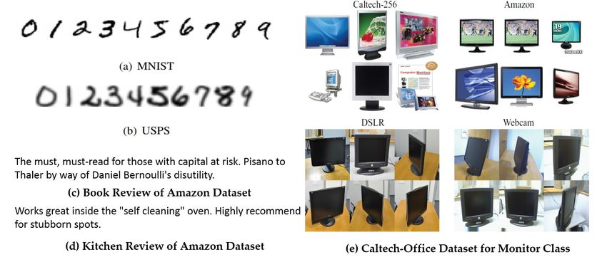
rarely encountered in real-world situations. For example, consider a recognition
system that distinguishes between a cat and a dog, given labelled training samples
of the type shown in Fig. 1(a). These training samples are frontal faces of cats and
dogs. When the same recognition system is used to test in a different domain such
as on the side images of cats and dogs as shown in Fig. 1(b), it would fail miser-
ably. This is because the recognition system has developed a bias in being able to
only distinguish between the face of a dog and a cat and not side images of dogs
and cats. Domain adaptation (DA) aims to mitigate this dataset bias (Torralba and
Efros, 2011), where different datasets have their own unique properties. Dataset

Figure 1: Discrepancy between the source domain and the target domain. In the source domain,
the images have frontal faces while the target domain has images of the whole body from the side
view-point.
bias appears because of the distribution shift of data from one dataset (i.e., source
domain) to another dataset (i.e., target domain). The distribution shift manifests
itself in different forms. In computer vision, it can occur when there is chang-
ing lighting conditions, changing poses, etc. In speech processing, it can be due
to changing accent, tone and gender of the person speaking. In remote sensing, it
can be due to changing atmospheric conditions, change in acquisition devices, etc.
To encounter this discrepancy in distributions, domain adaptation methods have
been proposed. Once domain adaptation is carried out, a model trained using the
adapted source domain data should perform well in the target domain. The under-
lying assumption in domain adaptation is that the task is the same in both domains.

                                               2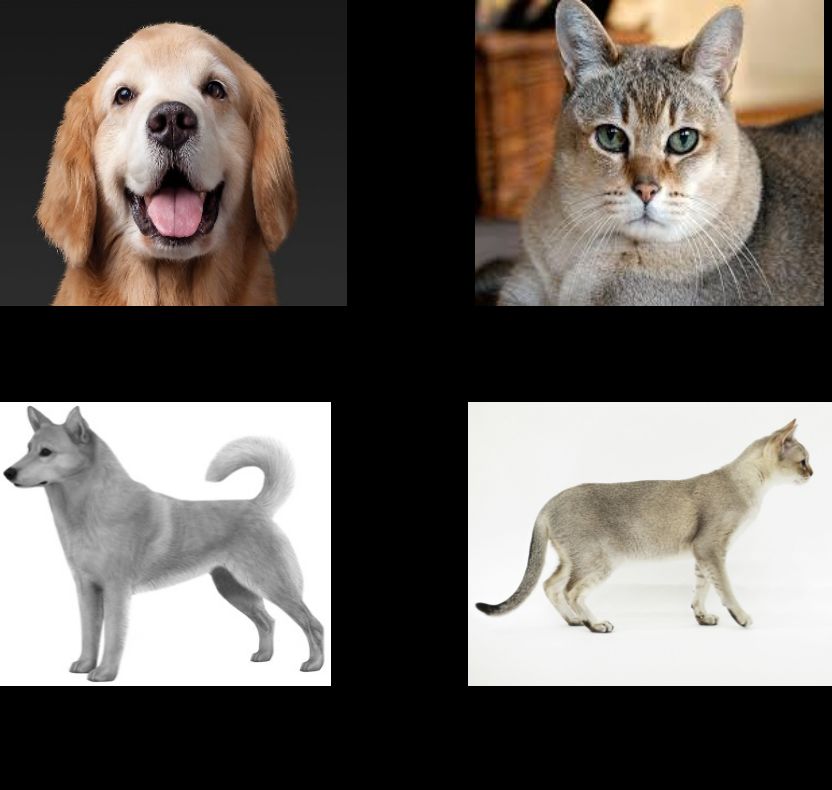
For classification problems, it implies that we have the same set of categories in
both source and target domains.
    Domain adaptation can also assist in annotating datasets efficiently and fur-
ther accelerating machine-learning research. Current machine-learning models
are data hungry and require lots of labelled samples. Though huge amount of un-
labelled data is obtained, labelling them requires lot of human involvement and
effort. Domain adaptation seeks to automatically annotate unlabelled data in the
target domain by adapting the labelled data in the source domain to be close to the
unlabeled target-domain data.
    In our work, we consider unsupervised domain adaptation (UDA), which as-
sumes absence of labels in the target domain. This is more realistic than semi-
supervised domain adaptation, where there are also a few-labelled data in the tar-
get domain. This is because labelling data might be time-consuming and expen-
sive for real-world situations. Hence we need to effectively exploit fully labelled
source-domain data and fully unlabelled target-domain data to carry out domain
adaptation. In our case, we seek to find correspondences between each source-
domain sample and each target-domain sample. Once the correspondences are
found, we can transform the source-domain samples to be close to the target-
domain samples. The transformed source-domain samples will then lie close to
the data space of the target domain. This will allow a model trained on the trans-
formed source-domain data to perform well with the target-domain data. This
not only achieves the goal of training robust models but also allows the model to
annotate unlabelled target-domain data accurately.
    The remainder of the paper is organized as follows: Section 2 discusses related
work of domain adaptation. Section 3 discusses the background required for our
proposed approach. Section 4 discusses our proposed approach and formulates
our unsupervised domain adaptation problem into a constrained convex optimiza-
tion problem. Section 5 discusses the experimental results and some comparison
with existing work. Section 6 discusses some limitations. Section 7 concludes
with a summary of our work and future research directions. Finally, the Appendix
shows more details about the proof of convexity of the optimization objective
function and derivation of the gradients.

2. Related Work
   There is a large body of prior work on domain adaptation. For our case, we
only consider homogeneous domain adaptation, where both the source and target

                                        3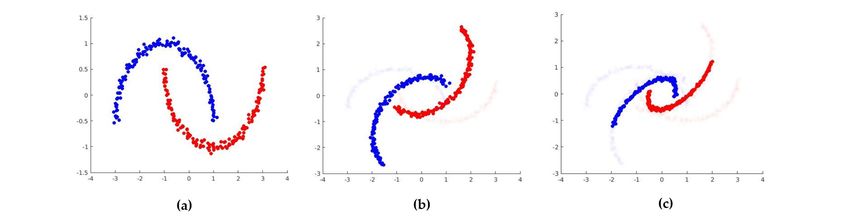
domains have the same feature space. Most of previous DA methods are classi-
fied into two categories, depending on whether a deep representation is learned
or not. In that regard, our proposed approach is not deep-learning-based since we
directly work at the feature level without learning a representation. We feel that
our method can easily be extended to deep architectures and provide much bet-
ter results. For a comprehensive overview on domain adaptation, please refer to
Csurka’s survey paper (Csurka, 2017).

2.1. Non-Deep-Learning Domain-Adaptation Methods
     These non-deep-learning domain-adaptation methods can be broadly classi-
fied into three categories – instance re-weighting methods, parameter adaptation
methods, and feature transfer methods. Parameter adaptation methods (Jiang
et al., 2008; Bruzzone and Marconcini, 2010; Duan et al., 2009; Yang et al., 2007)
generally adapt a trained classifier in the source domain (e.g., an SVM) in order to
perform better in the target domain. Since these methods require at least a small
set of labelled target examples, they cannot be applied to UDA.
     Instance Re-weighting was one of the early methods, where it was assumed
that conditional distributions were shared between the two domains. The in-
stance re-weighting involved estimating the ratio between the likelihoods of being
a source example or a target example to compute the weight of an instance. This
was done by estimating the likelihoods independently (Zadrozny, 2004) or by
approximating the ratio between the densities (Kanamori et al., 2009; Sugiyama
et al., 2008). One of the most popular measures used to weigh data instances,
used in (Gretton et al., 2009; Huang et al., 2007), was the Maximum Mean Dis-
crepancy (MMD) (Borgwardt et al., 2006) computed between the data distribu-
tions in the two domains. Feature Transfer methods, on the other hand, do not
assume the same conditional distributions between the source and target domains.
One of the simplest methods for DA was proposed in (Daumé III, 2009), where
the original representation is augmented with itself and a vector of the same size
is filled with zeros – the source features become (xs , xs , 0) and the target fea-
tures become (xt , 0, xt ). Then an SVM is trained on these augmented features to
figure out which parts of the representation is shared between the domains and
which are the domain-specific ones. The idea of feature augmentation inspires the
Geodesic Flow Sampling (GFS) (Gopalan et al., 2014, 2011) and the Geodesic
Flow Kernel (GFK) (Gong et al., 2012, 2013), where the domains are embedded
in d-dimensional linear subspaces that can be seen as points on the Grassman
manifold, corresponding to the collection of all d-dimensional subspaces. The
Subspace Alignment (SA) (Fernando et al., 2013) learns an alignment between the

                                         4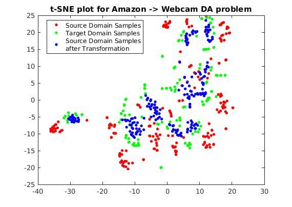
source subspace obtained by Principal Component Analysis (PCA) and the target
PCA subspace, where the PCA dimensions are selected by minimizing the Breg-
man divergence between the subspaces. Similarly, the linear Correlation Align-
ment (CORAL) (Sun et al., 2016) algorithm minimizes the domain shift using
the covariance of the source and target distributions. Transfer Component Anal-
ysis (TCA) (Pan et al., 2011) discovers common latent features having the same
marginal distribution across the source and target domains. Feature transforma-
tion proposed by (Chen et al., 2012) exploits the correlation between the source
and target sets to learn a robust representation by reconstructing the original fea-
tures from their noisy counterparts. All these previous methods learned a global
transformation between the source and target domains. In contrast, the Adaptive
Transductive Transfer Machines (ATTM) (Farajidavar et al., 2014) learned both a
global and a local transformation from the source domain to the target domain that
is locally linear. Similarly, the optimal transport for domain adaptation (Courty
et al., 2017) considers a local transport plan for each source example.

2.2. Deep Domain-Adaptation Methods
    Most deep-learning methods for DA follow a twin architecture with two streams,
representing the source and target models. They are then trained with a combina-
tion of a classification loss and a discrepancy loss (Long et al., 2016, 2015; Tzeng
et al., 2014; Ghifary et al., 2015; Sun and Saenko, 2016) or an adversarial loss.
The classification loss depends on the labelled source data, and the discrepancy
loss diminishes the shift between the two domains. On the other hand, adversarial-
based methods encourage domain confusion through an adversarial objective with
respect to a domain discriminator. The adversarial loss tries to encourage a com-
mon feature space through an adversarial objective with respect to a domain dis-
criminator. Tzeng et al. (2017) proposes a unified view of existing adversarial
DA methods by comparing them according to the loss type, the weight-sharing
strategy between the two streams, and on whether they are discriminative or gen-
erative. The Domain-Adversarial Neural Networks (DANN) (Ganin et al., 2016)
integrates a gradient reversal layer into the standard architecture to promote the
emergence of features that are discriminative for the main learning task in the
source domain and indiscriminate with respect to the shift between the domains.
The main disadvantage of these adversarial methods is that their training is gen-
erally not stable. Moreover, empirically tuning the capacity of a discriminator
requires lot of effort.
    Between these two classes of DA methods, the state-of-the-art methods are
dominated by deep architectures. However, these approaches are quite com-

                                         5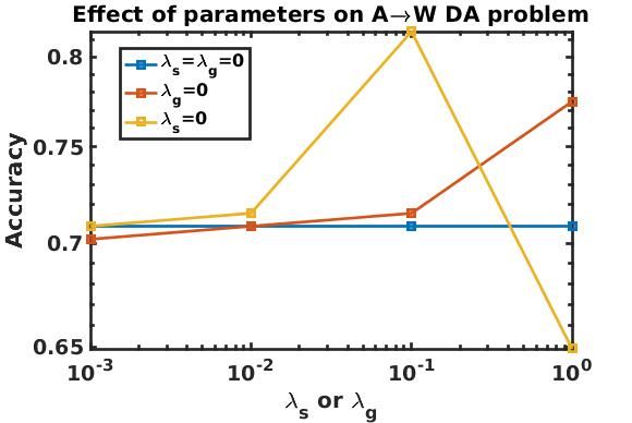
plex and expensive, requiring re-training of the network and tuning of many hy-
per parameters such as the structure of the hidden adaptation layers. Non-deep-
learning domain-adaptation methods do not achieve as good performance as a
deep-representation approach, but they work directly with shallow/deep features
and require lesser number of hyper-parameters to tune. Among the non-deep-
learning domain-adaptation methods, we feel feature transformation methods are
more generic because they directly use the feature space from the source and tar-
get domains, without any underlying assumption of the classification model. In
fact, a powerful shallow-feature transformation method can be extended to deep-
architecture methods, if desired, by using the features of each and every layer
and then jointly optimizing the parameters of the deep architectures as well as
that of the classification model. For example, correlation alignment (Sun et al.,
2016) has been extended for deep architectures (Sun and Saenko, 2016), which
evidently achieve the state-of-the art performance. Moreover, we believe a local
transformation-based approach as in (Courty et al., 2017; Farajidavar et al., 2014)
will result in better performance than global transformation methods because it
considers the effect of each and every sample in the dataset explicitly.

3. Background
    Our local transformation-based approach to DA places a strong emphasis on
establishing a sample-to-sample correspondence between each source-domain sam-
ple and each target-domain sample. Establishing correspondences between two
sets of visual features have long been used in computer vision mostly for im-
age registration (Besl and McKay, 1992; Chui and Rangarajan, 2003). To our
knowledge, the approach of finding correspondences between the source-domain
and the target-domain samples has never been used for domain adaptation. The
only work that is similar to finding correspondences is the work on optimal trans-
port (Courty et al., 2017). They learned a transport plan for each source-domain
sample so that they are close to the target-domain samples. Their transport plan
is defined on a point-wise unary cost between each source sample and each target
sample. Our approach develops a framework to find correspondences between the
source and target domains that exploit higher-order relations beyond these unary
relations between the source and target domains. We treat the source-domain data
and the target-domain data as the source and target hyper-graphs, respectively,
and our correspondence problem can be cast as a hyper-graph matching prob-
lem. The hyper-graph matching problem has been previously used in computer
vision (Duchenne et al., 2011) through a tensor-based formulation but has not

                                        6
been applied to domain adaptation. Hyper-graph matching involves using higher-
order relations between samples such as unary, pairwise, tertiary or more. Pair-
wise matching involves matching source-domain sample pairs with target-domain
sample pairs. Tertiary matching involves matching source-domain sample triplets
with target-domain sample triplets and so on. Thus, hyper-graph methods pro-
vide additional higher-order geometric and structural information about the data
that is missing with just using unary point-wise relations between a source sample
and a target sample. The advantage of using higher-order information in graph
Figure 2: Example showing the advantage of higher-order graph matching compared to just first-
order matching.
matching is demonstrated in the example in Fig. 2. In Fig. 2, the graph on the
left is constructed from the source domain while the graph on the right is con-
structed from the target domain. In the graph, each node represents a sample and
edges represent connectivity among the samples. Among these, samples 1 and 10
do not match because those samples are not the closest pair of samples. But as
a group {1, 2, 3} matches with {10 , 20 , 30 } suggesting that higher-order matching
can aid domain adaptation, whereas one-to-one matchings between samples might
not provide enough or provide incorrect information. Unfortunately, higher-order
graph matching comes with increasing computational complexity and also extra
hyper-parameters that weigh the importance of each of the higher-order relations.
Therefore , in our work we consider only the first-order and second-order match-
ings to validate the approach. Still, our problem can be inefficient because the
number of correspondence variables increases with the number of samples. To
address all these problems, we contribute in the following ways:
1. We initially propose a mathematical framework that uses the first-order
7and second-order relations to match the source-domain data and the target-
domain data. Once the relations are established, the source domain is mapped
to be close to the target domain. A class-based regularization is also used to
leverage the labels present in the source domain. All these cost factors are
combined into a convex optimization framework.
2. The above transformation approach is computationally inefficient. We then
reformulate our convex optimization problem into solving a series of sub-
problems for which an efficient solution using a network simplex approach.
This new formulation is more efficient in terms of both time and storage
space.
3. Finally, we have performed experimental evaluation of our proposed method
on both toy datasets as well as real image and sentiment classification datasets.
We have also examined the effect of each cost term in the convex optimiza-
tion problem separately.
The overall scheme of our proposed approach is shown in Fig. 3
Figure 3: Conceptual and high-level description of our proposed convex optimization formulation
with its proposed solution. The inputs are source-domain data (Xs ), source-domain labels (Ys ),
and target-domain data (Xt ). Output is a mapping function (M(·)) that maps Xs close to Xt . The
transformation can be repeated again by providing the transformed source data M(Xs ), source
labels Ys and target data Xt as input.
4. Proposed Sample-to-Sample Correspondence Method
In this section, we shall first define the domain adaptation problem (Pan and
Yang, 2010; Weiss et al., 2016), and then formulate the proposed correspondence-
and-mapping method for the unsupervised domain adaptation problem.
84.1. Notation
A domain is composed of a d-dimensional feature space X ⊂ Rd with a
marginal probability distribution P (X), and a task T defined by a label space
Y and the conditional probability distribution P (Y|X), where X and Y are ran-
dom variables. Given a particular sample set X = {x1 , . . . , xn } of X with cor-
responding labels Y = {y1 , . . . , yn } from Y, P (Y|X) can in general be learned
in a supervised manner from feature-label pairs {xi , yi }. For the domain adapta-
tion purpose, we assume that there are two domains with the same task: a source
domain Ds = {X s , P (Xs )} with T s = {Y s , P (Ys |Xs )} and a target domain
Dt = {X t , P (Xt )} with T t = {Y t , P (Yt |Xt )}. Traditional machine learning
techniques assume that both Ds = Dt and T s = T t , where Ds becomes the
training set and Dt the test set. For domain adaptation, Dt 6= Ds but T t = T s .
When the source domain is related to the target domain, it is possible to use the
relational information from Ds , T s to learn P (Yt |Xt ). The presence/absence of
labels in the target domain also decide how domain adaptation is being carried
out. We shall solve the most challenging case, where we have labelled source
domain data but unlabeled data in the target domain. This is commonly known
as unsupervised domain adaptation (UDA). A natural extension to UDA is the
semi-supervised case, where a small set of target domain samples is labelled.
In our case, we have labelled source-domain data with a set of training data
X = {xsi }ni=1
s s
associated with a set of class labels Ys = {yis }ni=1
s
. In the target do-
t nt
main, we only have unlabelled samples X = {xi }i=1 . If we had already trained a
t
classifier using the source-domain samples, the performance of the target-domain
samples on that classifier would be quite poor. This is because the distributions
of the source and target samples are different; that is, P (Xs ) 6= P (Xt ). So
we need to to find a transformation of the input space F : X s → X t such that
P (y|xt ) = P (y|F(xs )). As a result of this transformation, the classifier learned
on the transformed source samples can perform satisfactorily on the target-domain
samples.
4.2. Correspondence-and-Mapping Problem Formulation
With the above notation, our proposed approach considers the transformation
F as a point-set registration between two point sets, where the source samples
{xsi }ni=1
s
are the moving point set and the target samples {xti }ni=1
t
are the fixed
point set. In such a case, the registration involves alternately finding the corre-
spondence and mapping between the fixed and moving point sets (Chui and Ran-
garajan, 2003; Besl and McKay, 1992). The advantage of point-set registration
is that it ensures explicit sample-to-sample matching and not moment matching
9like covariance in CORAL (Sun et al., 2016) or MMD (Long et al., 2016, 2015;
Tzeng et al., 2014; Ghifary et al., 2015). As a result, the transformed source do-
main matches better with the target domain. However, matching each and every
sample requires an optimizing variable for each pair of source and target domain
samples. If the number of samples increases, so does the number of variables and
the optimization procedure may become extremely costly. We shall discuss how
to deal with the computational inefficiency later.
For the case when the number of target samples equals to the number of source
samples; that is, nt = ns , the correspondence can be represented by a permutation
matrix P ∈ {0, 1}ns ×nt . Element [P]ij = 1 if the source-domain sample xsi
corresponds to the target-domain
P sample xPj , and 0, otherwise. The permutation
t
matrix P has constraints i [P]ij = 1 and j [P]ij = 1 for all i ∈ {1, 2, . . . , ns }
and j ∈ {1, 2, . . . , nt }. Hence, if Xs ∈ Rns ×d and Xt ∈ Rnt ×d be the data matrix
of the source-domain and the target-domain data, respectively, then PXt permutes
the target-domain data matrix.
As soon as the correspondence is established, a linear or a non-linear mapping
must be established between the target samples and the corresponding source sam-
ples. Non-linear mapping is involved when there is localized mapping for each
sample, and it might also be required in case there is unequal domain shift of each
class. The mapping operation should map the source-domain samples as close
as possible to the corresponding target-domain samples. This process of finding
a correspondence between these transformed source samples and target samples
and then finding the mapping will continue iteratively till convergence. This it-
erative method of alternately finding the correspondence and mapping is similar
to feature registration in computer vision (Chui and Rangarajan, 2003; Besl and
McKay, 1992) but they have not been used or reformulated for unsupervised do-
main adaptation . In fact, the feature registration methods formulate the problem
as a non-convex optimization. Consequently, these methods suffer from local
minimum as in (Besl and McKay, 1992), and the global optimization technique
such as deterministic annealing (Chui and Rangarajan, 2003) does not guarantee
convergence. Thus, we propose to formulate it as a convex optimization problem
to obtain correspondences as a global solution. It is important to note that finding
such global and unique solution to the correspondence accurately is more impor-
tant because mapping with inaccurate correspondences will undoubtedly yield bad
results.
Formulating the proposed unsupervised domain adaptation problem as a con-
vex optimization problem requires the correspondences to have the following
10properties: (a) First-order similarity: The corresponding target-domain samples
should be as close as possible to the corresponding source-domain samples. This
implies that we want to have the permuted target-domain data matrix PXt to be
close to the source-domain data matrix Xs , which translates to minimizing the
Frobenius norm ||PXt − Xs ||2F in the least-squares sense . (b) Second-order
similarity: The corresponding target-domain neighborhood should be structurally
similar to the corresponding source-domain neighborhood. This structural simi-
larity can be expressed using graphs constructed from the source and target do-
mains. Thus, if the two domains can be thought of as weighted undirected graphs
Gs , Gt , structural similarity implies matching edges between the source and the
target graphs. The edges of these graphs can be expressed using the adjacency
matrices. If Ds and Dt are the adjacency matrices of Gs and Gt , respectively,
then these adjacency matrices can be found as,
||xsi − xsj ||22
[D ]ij = exp(−
s
)
σs2
||xti − xtj ||22
[Dt ]ij = exp(− )
σt2
[Ds ]ii = [Dt ]ii = 0,
where σs and σt can be found heuristically as the mean sample-to-sample pair-
wise distance in the source and target domains, respectively. For the second-order
similarity, we want the permuted target domain adjacency matrix PDt PT to be
close to the source domain adjacency matrix (region) Ds , where the superscript
T indicates a matrix transpose operation. We formulate it as equivalent to min-
imizing ||PDt PT − Ds ||2F . While this cost term geometrically implies the cost
of mis-matching edges in the constructed graphs, the first-order similarity term
can be thought as the cost of mis-matching nodes. However, the second-order
similarity cost term is bi-quadratic and we want to make it quadratic so that the
cost-function is convex and we can apply convex optimization techniques to it.
This can be done by post-multiplying PDt PT − Ds by P. Using the permutation
matrix properties PT P = I (orthogonal) and ||AP|| = ||A|| (norm-preserving),
this transformation produces the cost function ||PDt − Ds P||2F .
Estimating the correspondence as a permutation matrix in this quadratic set-
ting is NP-hard because of the combinatorial complexity of the constraint on
11P. We can relax the constraint on the correspondence matrix by converting it
from a discrete to a continuous form. The norms (i.e., Frobenius) used in the
cost/regularization terms will yield a convex minimization problem if we replace
P with a continuous constraint. Hence, if we relax the constraints on P to allow
for soft correspondences (i.e., replacing P with C), then an element of C matrix,
[C]ij , represents the probability that xsi corresponds to xtj . This matrix C is called
doubly stochastic matrix DB = {C ≥ 0 : C1 = CT 1 = 1} . DB represents
a convex hull, containing all permutation matrices at its vertices. (Birkhoff-von-
Neumann theorem).
In addition to the graph-matching terms, we add a class-based regularization
to the cost function that exploits the labelled informationPofP source-domain data.
The group-lasso regularizer `2 −`1 norm term is equal to j c ||[C]Ic j ||2 , where
|| · ||2 is the `2 norm and Ic contains the indices of rows of C corresponding to the
source-domain samples of class c. In other words, [C]Ic j is a vector consisting of
elements [C]ij , where ith source sample belongs to class c and the j th sample is in
the target domain. Minimizing this group-lasso term ensures that a target-domain
sample only corresponds to the source-domain samples that have the same label.
It is important to note that the solution to the relaxed problem may not be
equal or even close to the original discrete problem. Even then, the solution of the
relaxed problem need not be projected onto the set of permutation matrices to get
our final solution. This is because the graphs constructed using the source samples
and the target samples are far from isomorphic for real datasets. Therefore, we do
not expect exact matching between the nodes (samples) of each graph (domain)
and soft correspondences may serve better. As an example, consider that a source
sample xsi is likely to correspond to both xtj and xtk . In that case, it is more
appropriate to have correspondences [C]ij = 0.7 and [C]ik = 0.3 assigned to the
target samples, rather than the exact correspondences [C]ij = 1 and [C]ik = 0 or
vice-versa. Thus, we can formulate our optimization problem of obtaining C as
follows:
min f (C) =||CXt − Xs ||2F /(ns d)+ (1)
C
XX
λs ||CD − Ds C||2F + λg
t
||[C]Ic j ||2
j c
such that C ≥ 0, C1nt = 1ns , and CT 1ns = 1nt ,
where λs and λg are the parameters weighing the second-order similarity term and
class-based regularization term, respectively; 1ns and 1nt are column vectors of
12size ns and nt , respectively, and the superscript T indicates a matrix transpose
operation. The assumption that nt = ns is strict and it needs to be relaxed to
allow more realistic situations such as nt 6= ns . To analyze what modification is
required to the optimization problem in Eq. (1), we explore further to understand
the correspondences properly. In the case of nt = ns , we have one-to-one corre-
spondences between each source sample and each target sample. However, for the
case nt 6= ns , we must allow multiple correspondences. Initially, the constraint
C1nt = 1ns implies that the sum of the correspondences of all the target samples
to each source sample is one. The second equality constraint CT 1ns = 1nt implies
that the sum of correspondences of all the source samples to each target sample
is one. However, if nt 6= ns , the sum of correspondences of all the source sam-
ples to each target sample should increase proportionately by nnst to allow for the
multiple correspondences. This is reflected in the following optimization problem.
Problem UDA
nt s 2
min f (C) = ||CXt − Xs ||2F /(ns d) + λs ||CDt − ( )D C||F
C ns
(2)
XX
+ λg ||[C]Ic j ||2
j c
ns
such that C ≥ 0, C1nt = 1ns , and CT 1ns = ( )1nt
nt
for nt 6= ns .
4.3. Correspondence-and-Mapping Problem Solution
Problem UDA is a constrained convex optimization problem and can easily
be solved by interior-point methods (Boyd and Vandenberghe, 2004). In gen-
eral, the time complexity of these interior-point-methods for conic programming
is O(N 3.5 ), where N is the total number of the variables (Andersen, 2013). If we
have ns and nt as source and target samples, respectively, then the time complexity
becomes O(n3.5 s nt ). Also, the interior-point method is a second-order optimiza-
3.5
tion method. Hence, it requires storage space of the Hessian, which is O(N 2 ) ∼
O(n2s n2t ). This space complexity is more alarming and does not scale well with an
increasing number of variables. If nt and ns are greater than 100 points, it results
in memory/storage-deficiency problems in most personal computers. Thus, we
need to employ a different optimization procedure so that the proposed UDA ap-
proach can be widely used without memory-deficiency problem. We could think
13of first-order methods of solving the constrained optimization problem, which re-
quire computing gradients but do not require storing the Hessians.
First-order methods of solving the constrained optimization problem can be
broadly classified into projected-gradient methods and conditional gradient (CG)
methods (Frank and Wolfe, 1956). The projected-gradient method is similar to
the normal gradient-descent method except that for each iteration, the iterate is
projected back into the constraint set. Generally, the projected gradient-descent
method enjoys the same convergence rate as the unconstrained gradient-descent
method. However, for the projected gradient-descent method to be efficient, the
projection step needs to be inexpensive. With an increasing number of variables,
the projection step can become costly. Furthermore, the full gradient updating
may destroy the structure of the solutions such as sparsity and low rank. The con-
ditional gradient method, on the other hand, maintains the desirable structure of
the solution such as sparsity by solving the successive linear minimization sub-
problems over the convex constraint set. Since we expect our correspondence
matrix C to be sparse, we shall employ the conditional gradient method for our
problem. In fact, Jaggi (2013) points out that convex optimization problems over
convex hulls of atomic sets, which are relaxations of NP-hard problems are di-
rectly suitable for the conditional gradient method. This is similar to the way we
formulate our problem by relaxing P matrix to C.
Algorithm 1: Conditional Gradient Method (CG).
Given : C0 ∈ D, t = 1
Repeat
Cd = arg min Tr(∇C f (C0 )T C), such that C ∈ D
C
C1 = C0 + α(Cd − C0 ), for α = t+2 2
C0 = C1 and t = t + 1
Until Convergence or Fixed Number of Iterations
Output : C0 = arg min f (C) such that C ∈ D
C
As described in the above Algorithm 1 of the conditional gradient method, we
have to solve the linear programming problem, min Tr(∇C f (C0 )T C), such that
C
C ∈ D = {C : C ≥ 0, C1nt = 1ns , CT 1ns = ( nnst )1nt }. Here Tr(·) is the Trace
operator. The gradient ∇C f can be found from the equation:
∇C f = ∇C f1 /(ns d) + λs ∇C f2 + λg ∇C f3 , (3)
14P P
where f1 , f2 , and f3 are ||CXt −Xs ||2F , ||CDt −( nnst )Ds C||2F , and j c ||[C]Ic j ||2 ,
respectively.
The gradients are obtained as follows. The derivation is given in the Appendix
section-
∇C f1 = 2(CXt − Xs )(Xt )T
∇C f2 = 2CDt (Dt )T − 2rDs C(Dt )T − 2r(Ds )T CDt + 2r2 (Ds )T Ds C
where r = nt
ns
and
( [C]ij
∂f3 ||[C]Ic (i)j ||2
, if ||[C]Ic (i)j ||2 6= 0;
=
∂[C]ij 0, otherwise;
Here, c(i) is the class corresponding to the ith sample in the source domain and
Ic (i) contains the indices of source samples belonging to class c(i). After the
gradient ∇C f is found from ∇C f1 , ∇C f2 , ∇C f3 using Eq. 3, we need to solve
for the linear programming problem.
The linear programming problem can be solved easily using simplex methods
used in solvers such as MOSEK (Mosek, 2010). However, using such solvers
would not make our method competitive in terms of time efficiency. Hence, we
convert this linear programming problem into a min-cost flow problem, which can
then be solved very efficiently using a network simplex approach (Kelly, 1991).
Let the gradient ∇C f (C0 ) be G/ns and the correspondence matrix variable be
C = ns T. Then, the linear programming (LP) problem translates to min Tr(GT T)
T
such that T ≥ 0, T1nt = 1ns /ns , TT 1ns = 1nt /nt . This LP problem has an
equivalence with the min-cost flow problem on the following graph:
• The graph is bipartite with ns source nodes and nt sink nodes.
• The supply at each source node is 1/ns and the demand at each sink node is
1/nt .
• Cost of the edge connecting the ith source node to the j th sink node is given
by [G]ij . Capacity of each edge is ∞.
Using this configuration, the min-cost flow problem is solved using the network
simplex. Details of the network-simplex method is omitted and one can refer (Kelly,
151991). The network simplex method is an implementation of the traditional sim-
plex method for LP problems, where all the intermediate operations are performed
on graphs. Due to the structure of min-cost flow problems, network-simplex meth-
ods provide results significantly faster than traditional simplex methods. Using
this network-simplex method, we obtain the solution T∗ , where [T∗ ]ij is the flow
obtained on the edge connecting the ith source node to the j th sink node. From
that, we obtain Cd = ns T∗ and proceed with that iteration of conditional gradient
(CG) method as in Algorithm 1. In the above CG method, we also need an ini-
tial C0 and C0 can be defined as the solution to the LP problem, min Tr(DT C)
C
such that C ∈ D = {C : C ≥ 0, C1nt = 1ns , CT 1ns = ( nnst )1nt }, where
[D]ij = ||xsi − xtj ||2 . This is also solved by the network simplex approach after
converting this LP problem into its equivalent min-cost flow problem as described
previously. After we obtain C∗ from the CG algorithm, it is then used to find the
corresponding target samples Xtc = C∗ Xt . Then, the mapping M(·) from the
source domain to the target domain is found by solving the following regression
problem M(·) : X s → X t , with each row of Xs as an input data sample and the
corresponding row of Xtc as an output data sample. The choice of regressors can
be linear functions, neural networks, and kernel machines with proper regulariza-
tion. Once the mapping M∗ (·) is found out, a source-domain sample xs can be
mapped to the target domain by applying M∗ (xs ). This completes one iteration of
finding the correspondence and the mapping. For the next cycle, we solve Prob-
lem UDA with the mapped source samples as Xs and subsequently find the new
mapping. The number of iterations NT of alternatively finding correspondence
and mapping is an user-defined variable. The full domain adaptation algorithm is
outlined in Algorithm 2
Algorithm 2: Unsupervised Domain Adaptation using dataset registration.
Given : Source Labelled Data Xs and Ys , and Target Unlabelled Data Xt
Parameters : λs , λg , NT
Initialize : t = 0
Repeat
C∗ = argminf (C) such that C ∈ D (Find Correspondence using
CG method)
s M
Regress M(·) s.t. X − →C X ∗ t
(Find Mapping)
Map Xs = M(Xs ) and t = t + 1
Until t = NT
Output : Adapted Source Data Xs ,Ys to learn classifier.
165. Experimental Results and Discussions
To evaluate and validate the proposed sample-sample correspondence and map-
ping method for unsupervised domain adaptation, computer simulations were per-
formed on a toy dataset and then on image classification and sentiment classifi-
cation tasks. Our results were compared with previous published methods. For
comparisons, we used the reported accuracies or conduct experiments with the
available source code. Since we are dealing with unsupervised domain adapta-
tion, it is not possible to cross-validate our hyper-parameters λs , λg , and NT .
Unless explicitly mentioned, we reported the best results obtained over the hyper-
parameter ranges λs and λg in {10−3 , 10−2 , 10−1 , 100 , 101 , 102 , 103 } and NT = 1.
In our simulations, we found that using NT > 1 only provides a tiny bump in
performance or no improvement in performance at all. This is because the source
samples have already been transformed close to the target samples and further
transformation does not affect recognition accuracies. After the correspondence
was found, we considered mapping between the corresponding samples. For the
mapping, we used a linear mapping W ∈ Rd×d with a regularization of 0.001. d
is the dimension of the feature space in which the data lies.
Figure 4: (a) Source-domain data. (b) Target-domain data consists of a 50-degree rotation of the
source-domain data. (c) Transformed source-domain data is now aligned with the target-domain
data.
5.1. Toy Dataset: Two interleaving moons
For the first experiment, we used the synthetic dataset of interleaving moons
previously used in (Courty et al., 2017; Germain et al., 2013). The dataset consists
of 2 domains. The source domain consists of 2 entangled moon’s data. Each moon
is associated with each class. The target domain consists of applying a rotation to
the source domain. This can be considered as a domain-adaptation problem with
increasing rotation angle implying increasing difficulty of the domain-adaptation
17Table 1: Accuracy results over 10 trials for the toy dataset domain-adaptation problem for varying
degree of rotation between source and target domain
Angle (◦ ) 10 20 30 40 50 70 90
SVM-NA 100 89.6 76.0 68.8 60.0 23.6 17.2
DASVM 100 100 74.1 71.6 66.6 25.3 18.0
PBDA 100 90.6 89.7 77.5 59.8 37.4 31.3
OT-exact 100 97.2 93.5 89.1 79.4 61.6 49.3
OT-IT 100 99.3 94.6 89.8 87.9 60.2 49.2
OT-GL 100 100 100 98.7 81.4 62.2 49.2
OT-Laplace 100 100 99.6 93.8 79.9 59.8 47.6
Ours 100 100 96 87.4 83.9 78.4 72.2
problem. Since the problem is low dimensional, it allowed us to visualize the
effect of our domain-adaptation method appropriately. Figures 4(a) and 4(b) show
an example of the source-domain data and the target-domain data respectively, and
Fig. 4(c) shows the adapted source-domain data using the proposed approach. The
results showed that the transformed source domain becomes close to the target
domain.
For testing on this toy dataset, we used the same experimental protocol as
in (Courty et al., 2017; Germain et al., 2013). We sampled 150 instances from the
source domain and the same number of examples from the target domain. The test
data was obtained by sampling 1000 examples from the target domain distribution.
The classifier used is an SVM with a Gaussian kernel, whose parameters are set
by 5-fold cross-validation. The experiments were conducted over 10 trials and the
mean accuracy was reported. At this juncture, it is important to note that choosing
the classifier for domain adaptation is important. For example, the two classes
in the interleaving moon dataset are not linearly separable at all. So, a linear
kernel SVM would not classify the moons accurately and it would result in poor
performance in the target domain as well. That is why we need a Gaussian Kernel
SVM. So, we have to make sure that we choose a classifier that works well with
the source dataset in the first place.
We compared our results with the DA-SVM (Bruzzone and Marconcini, 2010)-
a domain-adaptive support vector machine approach, PBDA (Germain et al., 2013)-
which is a PAC-Bayesian based domain adaptation method, and different versions
of the optimal transport approach (Courty et al., 2017). OT-exact is the basic op-
timal transport approach. OT-IT is the information theoretic version with entropy
regularization. OT-GL and OT-Laplace has additional group and graph based reg-
18Table 2: Time comparison (in seconds) of the two solvers for increasing sample size. The sample
size is the number of samples per class per domain of the interleaving moon toy dataset. The target
domain has a rotation of 50◦ with the source domain. We use NT = 1. Implementation was in
MATLAB in a workstation with Intel Xeon(R) CPU E5-2630 v2 and 40 GB RAM. Results are
reported over 10 trials.
n 25 50 75 100 125 150 175 200
M 62.1 83.1 103.4 128.5 387.7 680.1 1028.3 1577.6
N-S 1.5 4 6.9 10.1 16.9 23.5 31.2 41.3
ularization, respectively. From our results in Table 1, we see that for low rotation
angles, the OT-GL-based method dominates and our proposed method yields sat-
isfactory results. But for higher angles (≥ 50 ◦ ), our proposed method clearly
dominates by a large margin. This is because we have taken into consideration
second-order structural similarity information. For higher-rotation angles, the
point-to-point sample distance is high. However, similar structures in the source
and target domains can still correspond to each other. In other words, the adja-
cency matrices, which depend on relative distances between samples, can still be
matched and do not depend on higher rotation angles between the source and tar-
get domains. That is why our proposed method out-performed other methods for
large discrepancies between the source and target distributions.
We further provided the time comparison between the network simplex method
(N-S) and MOSEK (M) for increasing number of samples of the toy dataset in Ta-
ble 2. Results showed that the network simplex method is very fast compared to a
general purpose linear programming solver like MOSEK.
5.2. Real Dataset: Image Classification
We next evaluated the proposed method on image classification tasks. The
image classification tasks that we considered were digit recognition and object
recognition. The classifier used was 1-NN (Nearest Neighbor). 1-NN is used
for experiments with images because it does not require cross-validating hyper-
parameters and has been used in previous work as well (Courty et al., 2017; Gong
et al., 2012) The 1-NN classifier is trained on the transformed source-domain data
and tested on the target-domain data. Instances of the image dataset are shown
in Fig. 5 (a),(b) and (e). Generally, we cannot directly cross-validate our hyper-
parameters λs and λg on the unlabelled target domain data making it impractical
for real-world applications. However, for practical transfer learning purposes,
a reverse validation (RV) technique(Zhong et al., 2010) was developed for tun-
19Figure 5: Instances of the real dataset used. At the top left, we see that USPS has the worse
resolution compared to MNIST handwriting dataset. At the bottom left, we have instances of the
Amazon review dataset. There is a shift in textual domain when reviewing for different prod-
ucts. On the right, we have the Caltech-Office dataset and we see that there are differences in
illumination, quality, pose, presence/absence of background across different domains.
ing the hyper-parameters. We have carried out experiments with a variant of the
method to tune λs and λg for our UDA approach..
For a particular hyper-parameter configuration, we divide the source domain
data into K folds. We use one of the folds as the validation set. The remaining
source data and the whole target data are used for domain adaptation. The clas-
sifier trained using the adapted source data is used to generate pseudo-labels for
the target data. Another classifier is trained using the target domain data and its
pseudo-labels. This classifier is then tested on the held-out source domain data
after adaptation. The accuracy obtained is repeated and averaged over all the K
folds. This reverse-validation approach is repeated over all hyper-parameter con-
figurations. The optimal hyper-parameter configuration is the one with the best
average validation accuracy. Using the obtained optimal hyper-parameter config-
uration, we then carry out domain adaptation over all the source and target do-
main data and report the accuracy over the target domain dataset. We used K = 5
folds for all the real-data experiments. Thus, we showed the results using this RV
approach in addition to the best obtained results over the hyper-parameters. In
majority of the cases in Tables 3,5,6 and 7 we would see that the result obtained
using the reverse validation approach matches the best obtained results suggesting
that the hyper-parameters can be automatically tuned successfully.
205.2.1. Digit Recognition
For the source and target domains, we used 2 datasets – USPS (U) and MNIST
(M). These datasets have 10 classes in common (0-9). The dataset consists of
randomly sampling 1800 and 2000 images from USPS and MNIST, respectively.
The MNIST digits have 28 × 28 resolution and the USPS 16 × 16. The MNIST
images were then resized to the same resolution as that of USPS. The grey levels
were then normalized to obtain a common 256-dimensional feature space for both
domains.
5.2.2. Object Recognition
For object recognition, we used the popular Caltech-Office dataset (Gong
et al., 2012; Gopalan et al., 2011; Saenko et al., 2010; Zheng et al., 2012; Courty
et al., 2017). This domain-adaptation dataset consists of images from 4 differ-
ent domains: Amazon (A) (E-commerce), Caltech-256 (Griffin et al., 2007) (C)
(a repository of images), Webcam (W) (webcam images), and DSLR (D) (images
taken using DSLR camera). The differences between domains are due to the dif-
ferences in quality, illumination, pose and also the presence and absence of back-
grounds. The features used are the shallow SURF features (Bay et al., 2006) and
deep-learning feature sets (Donahue et al., 2014) – decaf6 and decaf7. The SURF
descriptors represent each image as a 800-bin histogram. The histogram is first
normalized to represent a probability and then reduced to standard z-scores. On
the other hand, the deep-learning feature sets, decaf6 and decaf7, are extracted as
the sparse activation of the neurons from the fully connected 6th and 7th layers
of convolutional network trained on imageNet and fine tuned on our task. The
features are 4096-dimensional.
For our experiments, we considered a random selection of 20 samples per class
(with the exception of 8 samples per class for the DSLR domain) for the source
domain. The target-domain data is split equally. One half of the target-domain
data is used for domain adaptation and the other half is used for testing. This is
in accordance with the protocol followed in (Courty et al., 2017). The accuracy is
reported on the test data over 10 trials of the experiment.
We compared our approach against (a) the no adaptation baseline (NA), which
consists of using the original classifier without adaptation; (b) Geodesic Flow
Kernel (GFK) (Gong et al., 2012); (c) Transfer Subspace Learning (TSL) (Si
et al., 2010), which minimizes the Bregman divergence between low-dimensional
embeddings of the source and target domains; (d) Joint Distribution Adaptation
(JDA) (Long et al., 2013), which jointly adapts both marginal and conditional
distributions along with dimensionality reduction; (e) Optimal Transport (Courty
21et al., 2017) with the information-theoretic (OT-IT) and group-lasso version (OT-
GL). Among all these methods, TSL and JDA are moment-matching methods
while OT-IT, OT-GL and ours are sample-matching methods.
The best performing method for each domain-adaptation problem is high-
lighted in bold. From Table 3, we see that in almost all the cases, the OT-GL
and our proposed method dominated over other methods, suggesting that sample-
matching methods perform better than moment-matching methods. For the hand-
written digit recognition tasks (U → M and M → U), our proposed method clearly
out-performs GFK, TSL and JDA, but is slightly out-performed by OT-GL. This
might be because the handwritten digit datasets U and M do not contain enough
structurally similar regions to exploit the second-order similarity cost term. For
the Office-Caltech dataset, the only time our proposed method was beaten by a
moment-matching method was W → D, though by a slight amount. This is be-
cause W and D are closest pair of domains and using sample-based matching does
not have outright advantage over moment-matching. The fact that W and D have
the closest pair of domains is evident form the NA accuracy of 53.62, which is the
best among NA accuracies of the Office-Caltech domain-adaptation tasks.
We have performed a runtime comparison in terms of the CPU time in sec-
onds of our method with other methods and have shown the results in Table 4.
The experiments performed are over the same dataset as used in Table 3. From
Table 4, we see that local methods like OT-GL and our method generally take
more time than moment-matching method like JDA. Our method takes more time
compared with OT-GL because of time taken in constructing adjacency matrices
for the second order cost term. Overall, the time taken for domain adaptation be-
tween USPS and MNIST datasets is more because they contain relatively larger
number of samples, compared to the Office-Caltech dataset.
We have also reported the results of Office-Caltech dataset using decaf6 and
decaf7 features in Tables 5 and 6, respectively. The baseline performance of the
deep-learning features are better than SURF features because they are more robust
and contain higher-level representations. Expectedly, the decaf7 features have bet-
ter baseline performance than decaf6 features. However, DA methods can further
increase performance over the robust deep features. In Tables 5 and 6, we see
that our proposed method dominates over JDA and OT-IT but is in close competi-
tion with OT-GL. We also noted that using decaf7 instead of decaf6 creates only
a small incremental improvement in performance because most of the adaptation
has already been performed by our proposed domain-adaptation method. As seen
in Fig. 6, the source-domain samples are transformed to be near the target-domain
samples using our proposed method. Therefore, we expect a classifier trained on
22Table 3: Domain-adaptation results for digit recognition using USPS and MNIST datasets and
object recognition with the Office-Caltech dataset using SURF features.
Tasks NA GFK TSL JDA OT-GL Ours Ours (RV)
U→M 39.00 44.16 40.66 54.52 57.85 56.90 56.90
M→U 58.33 60.96 53.79 60.09 69.96 68.44 66.24
C→A 20.54 35.29 45.25 40.73 44.17 46.67 46.67
C→W 18.94 31.72 37.35 33.44 38.94 39.48 39.48
C→D 19.62 35.62 39.25 39.75 44.50 42.88 40.12
A→C 22.25 32.87 38.46 33.99 34.57 38.51 38.51
A→W 23.51 32.05 35.70 36.03 37.02 38.69 38.69
A→D 20.38 30.12 32.62 32.62 38.88 36.12 36.12
W→C 19.29 27.75 29.02 31.81 35.98 33.81 32.83
W→A 23.19 33.35 34.94 31.48 39.35 37.69 37.69
W→D 53.62 79.25 80.50 84.25 84.00 84.10 84.10
D→C 23.97 29.50 31.03 29.84 32.38 32.78 32.78
D→A 27.10 32.98 36.67 32.85 37.17 38.33 37.61
D→W 51.26 69.67 77.48 80.00 81.06 81.12 81.12
Table 4: CPU time (seconds) comparison of different domain adaptation algorithms.
Task NA GFK TSL JDA OT-GL Ours
U→M 1.24 2.62 567.8 82.34 171.84 201.23
M→U 1.13 2.43 522.37 81.13 168.23 196.15
C→A 0.46 2.6 382.98 41.6 85.95 99.9
C→W 0.24 1.45 157.52 37.89 78.73 101.1
C→D 0.36 1.35 117.81 37.33 61.17 63.38
A→C 0.54 2.69 462.12 40.11 105.87 126.18
A→W 0.39 1.47 153.95 37.63 86.12 100.21
A→D 0.42 1.31 115.87 36.82 69.29 82.1
W→C 0.33 2.92 461.1 42.39 98.26 111.2
W→A 0.61 2.52 388.23 41.64 94.38 101.45
W→D 0.34 1.37 117.47 37.9 76.5 79.25
D→C 0.45 2.36 364.13 39.75 106.21 118.12
D→A 0.43 2.14 310.18 41.24 98.41 115.35
D→W 0.24 1.05 93.73 34.62 76.23 88.69
23Table 5: Domain-adaptation results for the Office-Caltech dataset using decaf6 features.
Task NA JDA OT IT OT-GL Ours Ours(RV)
C→A 79.25 88.04 88.69 92.08 91.92 89.91
C→W 48.61 79.60 75.17 84.17 83.58 81.23
C→D 62.75 84.12 83.38 87.25 87.50 87.50
A→C 64.66 81.28 81.65 85.51 86.67 85.63
A→W 51.39 80.33 78.94 83.05 81.39 81.39
A→D 60.38 86.25 85.88 85.00 87.12 87.12
W→C 58.17 81.97 74.80 81.45 82.13 81.64
W→A 61.15 90.19 80.96 90.62 88.87 88.87
W→D 97.50 98.88 95.62 96.25 98.95 98.95
D→C 52.13 81.13 77.71 84.11 83.72 83.72
D→A 60.71 91.31 87.15 92.31 92.65 92.65
D→W 85.70 97.48 93.77 96.29 96.69 96.13
Table 6: Domain-adaptation results for the Office-Caltech dataset using decaf7 features.
Task NA JDA OT-IT OT-GL Ours Ours(RV)
C→A 85.27 89.63 91.56 92.15 91.85 91.85
C→W 65.23 79.80 82.19 83.84 85.36 85.36
C→D 75.38 85.00 85.00 85.38 85.88 85.88
A→C 72.80 82.59 84.22 87.16 86.67 85.39
A→W 63.64 83.05 81.52 84.50 86.09 85.36
A→D 75.25 85.50 86.62 85.25 87.37 87.37
W→C 69.17 79.84 81.74 83.71 82.80 82.80
W→A 72.96 90.94 88.31 91.98 90.15 89.31
W→D 98.50 98.88 98.38 91.38 99.00 99.00
D→C 65.23 81.21 82.02 84.93 82.20 82.20
D→A 75.46 91.92 92.15 92.92 92.60 92.15
D→W 92.25 97.02 96.62 94.17 97.10 97.10
24Figure 6: t-SNE (Maaten and Hinton, 2008) visualization of a single trial of Amazon to Webcam
DA problem using decaf6 features.
the transformed source samples to perform better on the target-domain data.
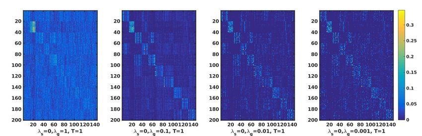
We have also studied the effects of varying the regularization parameters on
domain-adaptation performance. In Fig. 7, the blue line shows the accuracy when
both λs = λg = 0. When λs = 0, best performance is obtained for λg = 0.1.
When λg = 0, best performance is obtained for λg = 1. For λs , λg > 1, per-
formance degrades (not shown) because we have put excess weight on the regu-
larization terms of second-order structural similarity and group-lasso than on the
first-order point-wise similarity cost term. Thus, the presence of second-order and
regularization term, weighted in the right amount is justified as it improves per-
formance over when only the first-order term is present. We have also studied
the effect of group-lasso regularization parameter (λg ) on the quality of the corre-
spondence matrix C obtained for a domain-adaptation task. Visually the second
plot from the left in Fig. 8 appears to discriminate the 10 classes best. Accord-
ingly, this parameter configuration (λs = 0, λg = 0.1, NT = 1) realizes the best
performance as shown in the previous Fig. 7.
25Figure 7: Effect of varying regularization parameters λs and λg on the accuracy of Amazon (source
domain) to Webcam (target domain) visual domain-adaptation problem for fixed NT = 1.
Figure 8: The optimal correspondence matrix C for 4 different parameter settings visualized as
a colormap, with λs = 0, NT = 1. The task involved was the Amazon to Webcam domain
adaptation.
265.3. Real Dataset: Sentiment Classification
We have also evaluated our proposed method on sentiment classification using
the standard Amazon review dataset (Blitzer et al., 2007). This dataset contains
Amazon reviews on 4 domains: Kitchen items (K), DVD (D), Books (B) and Elec-
tronics (E). Instances of the dataset are shown in Fig. 5 (c),(d). The dimensionality
of the bag-of-word features was reduced by keeping the top 400 features having
maximum mutual information with class labels. This pre-processing was also car-
ried out in (Sun et al., 2016; Gong et al., 2013) without losing performance. For
each domain, we used 1000 positive and 1000 negative reviews. For each domain-
adaptation task, we used 1600 samples (800 positive and 800 negative) from each
domain as the training dataset. The remaining 400 samples (200 positive and 200
negative) were used for testing. The classifier used is a 1-NN classifier since it
is parameter free. The mean-accuracy was reported over 10 random training/test
splits.
We compared our proposed approach to a recently proposed unsupervised
domain-adaptation approach known as Correlation Alignment (CORAL) (Sun
et al., 2016). CORAL is a simple and efficient approach that aligns the input
feature distributions of the source and target domains by exploring their second-
order statistics. Firstly, it computes the covariance statistics in each domain and
then applies whitening and re-coloring linear transformation to the source fea-
tures. Results in Table 7 showed that our proposed method outperforms CORAL
in all the domain-adaptation tasks. Our proposed method has better performance
because CORAL matches covariances while our method matches samples explic-
itly through point-wise and pair-wise matching. Moreover, CORAL does not use
source-domain label information. Our method uses source-domain label infor-
mation through the group-lasso regularization. However, CORAL is quite fast
in transforming the source samples compared to our method. For a single trial,
CORAL took about a second while our proposed method took about a few min-
utes.
Table 7: Accuracy results of unsupervised domain-adaptation tasks for the Amazon reviews
dataset.
Tasks K→D D→B B→E E→K K→B D→E
NA 58.6 63.4 58.5 66.5 59.3 57.9
CORAL 59.9 66.5 59.5 67.5 59.2 59.5
Ours 63.5 69.5 62.0 69.5 64.5 61.2
Ours (RV) 60.9 69.5 62.0 69.5 64.5 59.0
27You can also read