A Comparative Analysis of Different Future Weather Data for Building Energy Performance Simulation - MDPI
←
→
Page content transcription
If your browser does not render page correctly, please read the page content below
climate
Article
A Comparative Analysis of Different Future Weather Data for
Building Energy Performance Simulation
Mamak P.Tootkaboni 1, * , Ilaria Ballarini 1 , Michele Zinzi 2                             and Vincenzo Corrado 1

                                          1   Department of Energy, Politecnico di Torino, 10129 Turin, Italy; ilaria.ballarini@polito.it (I.B.);
                                              vincenzo.corrado@polito.it (V.C.)
                                          2   ENEA, Via Anguillarese 301, 00123 Rome, Italy; michele.zinzi@enea.it
                                          *   Correspondence: mamak.ptootkaboni@polito.it

                                          Abstract: The building energy performance pattern is predicted to be shifted in the future due to
                                          climate change. To analyze this phenomenon, there is an urgent need for reliable and robust future
                                          weather datasets. Several ways for estimating future climate projection and creating weather files
                                          exist. This paper attempts to comparatively analyze three tools for generating future weather datasets
                                          based on statistical downscaling (WeatherShift, Meteonorm, and CCWorldWeatherGen) with one
                                          based on dynamical downscaling (a future-typical meteorological year, created using a high-quality
                                          reginal climate model). Four weather datasets for the city of Rome are generated and applied to the
                                          energy simulation of a mono family house and an apartment block as representative building types
                                          of Italian residential building stock. The results show that morphed weather files have a relatively
                                          similar operation in predicting the future comfort and energy performance of the buildings. In
                                          addition, discrepancy between them and the dynamical downscaled weather file is revealed. The
                                analysis shows that this comes not only from using different approaches for creating future weather

                                          datasets but also by the building type. Therefore, for finding climate resilient solutions for buildings,
Citation: P.Tootkaboni, M.; Ballarini,    care should be taken in using different methods for developing future weather datasets, and regional
I.; Zinzi, M.; Corrado, V. A              and localized analysis becomes vital.
Comparative Analysis of Different
Future Weather Data for Building
                                          Keywords: climate change; future weather data; building energy performance; thermal comfort;
Energy Performance Simulation.
                                          statistical downscaling of climate models; dynamical downscaling of climate models
Climate 2021, 9, 37. https://doi.org/
10.3390/cli9020037

Academic Editor: Steven McNulty
                                          1. Introduction
Received: 2 February 2021                      There is an urgent need to address climate change as a primary global problem.
Accepted: 19 February 2021                According to the World Meteorological Organization (WMO) report on global climate,
Published: 23 February 2021               recent years have seen a continued increase in greenhouse gas concentration, global mean
                                          temperature, global sea level, and melting cryosphere [1]. The fifth assessment report (AR5)
Publisher’s Note: MDPI stays neutral      of the Intergovernmental Panel on Climate Change (IPCC) points out that if the emissions
with regard to jurisdictional claims in   continue to rise, the global average temperature will be 2.6-4.8 degrees Celsius (◦ C) higher
published maps and institutional affil-   than the present by the end of the 21st century. Even if the greenhouse gas emissions stop
iations.                                  immediately, the temperature increase will persist for centuries due to the effect of already
                                          present greenhouse gases in the atmosphere [2].
                                               In addition to the changes in average temperature trend, extreme events intensify in
                                          frequency and magnitude; as an example, over the period 1880 to 2005, the frequency of
Copyright: © 2021 by the authors.         heat waves in Europe has doubled, and longer heatwaves are more than 90% definite as
Licensee MDPI, Basel, Switzerland.        the climate pattern has been disrupted [3]. The August 2003 heatwave was responsible for
This article is an open access article    around 45,000 excess deaths across 12 European countries [4]. From 2015 to 2019, heatwaves
distributed under the terms and           were the deadliest meteorological hazard in many countries, particularly in Europe and
conditions of the Creative Commons        North America [1], with an increase of mortality [5] and morbidity, especially for the
Attribution (CC BY) license (https://     elderly [6]. Consequences of these extremes included higher energy uses in buildings [5–7],
creativecommons.org/licenses/by/          infrastructure failures [8,9], and negative economic impacts [10,11].
4.0/).

Climate 2021, 9, 37. https://doi.org/10.3390/cli9020037                                                            https://www.mdpi.com/journal/climate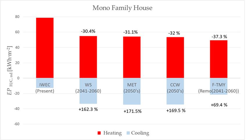
Climate 2021, 9, 37                                                                                            2 of 16

                            Future climate scenarios affirm these trends, projecting different warming rates built
                      upon a number of possible scenarios of future anthropogenic greenhouse gas emissions.
                      The first set of scenarios was Emissions Scenarios (SRES), which were introduced in the
                      IPCC 4th Special Report in 1996 [12]. Later, in 2014, the IPCC adopted a new series of
                      scenarios called “Representative Concentration Pathways (RCPs)” that are established
                      using hypotheses about economic growth, choices of technology, and land use [2]. RCPs
                      are identified by their associated warming effect (radiative forcing, which is measured in
                      units of watts per meter squared) in the year 2100. Radiative forcing is a direct measure
                      of the amount Earth’s energy imbalance. The four RCPs (RCP2.6, RCP4.5, RCP6.0, and
                      RCP8.5) span a range of assumptions about future controls on greenhouse gas (and other)
                      emissions. The lowest RCP represents a very aggressive Green House Gases (GHG) mit-
                      igation scenario aimed at limiting global warming to about 2 ◦ C, while the highest RCP
                      corresponds to minimal effort to reduce GHG emissions this century. The RCP 8.5 assumes
                      that atmospheric concentrations of CO2 are three to four times higher than pre-industrial
                      levels by 2100 [2].
                            Insights from these future scenarios demonstrate the urgent need for emission reduc-
                      tion in a wide range of relevant sectors. Among these sectors, the building stock is one of
                      the main greenhouse gas emitters, which in the European Union accounts for 50% of the
                      CO2 emissions [13]. In addition, buildings will be also subjected to a warmer climate due to
                      their long lifespan. The existing body of research on the effect of climate change on the fu-
                      ture performance of buildings predicts that there will be a paradigm shift in building energy
                      performance. Unsurprisingly, a drastic rise in cooling energy use and a moderate decrease
                      in heating energy use is predicted [14–16]. Recently, in the study of Soutullo et al. [17], for
                      two reference buildings in Madrid, the annual heating and cooling requirements were
                      shown to be around 22% lower and higher, respectively, just by considering the effect of
                      climate change in the last decade. In addition, many studies revealed that this trend may
                      happen even in energy efficient dwellings. Da Guarda et al. [18] analyzed the vulnerability
                      of a zero-energy building (ZEB) to the impact of climate change in 2020 (2011 to 2040),
                      2050 (2041 to 2070), and 2080 (2071 to 2100). Results showed that due to the increase in
                      cooling energy consumption, there will be a power generation gap up to 40.2% for the
                      2080 period. In addition, the climate change impact magnitude is not equal for different
                      scenarios, case studies, and regions. Zhai and Helman [19] studied a campus building
                      stock energy prediction, using four future climate models, which are representative of
                      56 model scenarios for seven climate zones in US. The results demonstrated that cooling
                      energy increases variously (5%, 28%, 20%, and 52%) for different scenarios. In another
                      study, Chai et al. [20] analyzed the life cycle of a net zero energy building in typical climate
                      regions of China. It was concluded that among the different climate regions, the impact
                      of climate change on energy balance and thermal comfort varies significantly. So, in a
                      changing climate, it becomes necessary to prepare buildings for the future at the regional
                      scale, considering different scenarios, to avoid problems such as overheating and power
                      outage, which brings health risks for the occupants.
                            To investigate the future performance of a building in the context of climate change,
                      building energy simulation (BES) is a vital support tool. BES needs a robust weather
                      dataset that defines the external boundary conditions the building will face during its
                      lifetime. Typically, a representative year of hourly weather data is required to represent
                      the typical regional climate condition and to define the dynamic energy behavior of the
                      building. Several methodologies have been developed to create this one-year climate
                      data from historical climate records [21]. The most commonly used methodology is the
                      Typical meteorological year (TMY), which was introduced in 1978 [22]. TMY is a fictive
                      year constructed of twelve representative typical months [23]. Representative months
                      are selected by comparing the distribution of each month with the long-term distribution
                      of that month for the available climate dataset (the Finkelstein–Schafer statistics) [24].
                      The analysis of the present climate is based on the observation of climate variables and
                      the application of statistical methods for understanding the current trends. On the other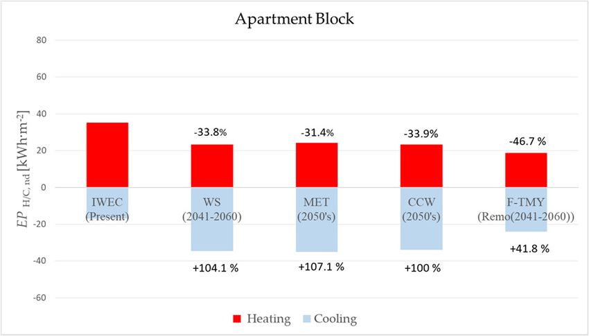
Climate 2021, 9, 37                                                                                           3 of 16

                      hand, the analysis of future climate is based on future scenarios and the projections of
                      climate models.
                             Future scenarios are the input data used to provide initial conditions for General
                      Circulation Models or Global Climate Models (GCMs), which are models for forecasting
                      climate change. GCMs provide climate information on the global scale with a typical
                      spatial resolution of 150–600 km2 [2]. Consequently, if they are used for building energy
                      simulation, the climate change effect and related weather extremes at the local level will
                      not be considered. In this case, the GCMs should be downscaled to applicable spatial
                      (less than 100 km2 ) and temporal resolution (less than monthly value). There are two
                      main approaches to downscale GCMs: dynamical and statistical downscaling. Several
                      studies compared different methodologies that use these approaches for the generation of
                      future weather data. Jentsch et al. indicate that weather variability is not generated in the
                      statistically downscaled weather dataset and this approach includes the effect of climate
                      change independently between the variables [25]. On the other hand, Dias et al. point out
                      that the statistical downscaling approach has the advantage of reducing the computational
                      time so that various climate change scenarios can be applied [26], besides providing enough
                      information to study the performance of the building [27]. In light of these studies, there is
                      still a need to deeply analyze different methodologies for future weather data generation.
                             This study aims to contribute to evaluating the suitability and robustness of different
                      future weather data for analyzing the future performance of reference buildings both in
                      terms of thermal comfort and energy performance. It represents a comparative study
                      of four future weather datasets. Three of them were produced using common weather
                      generator tools available today (WeatherShift, Meteonorm, and CCWorldWeatherGen),
                      which apply statistical downscaling. The other one is a TMY created using a high-quality
                      regional climate models database (from Euro-Coordinated Regional Climate Downscaling
                      Experiment (CORDEX)) that applies the dynamical downscaling. The study investigates
                      the impact of each type of these future weather data in the building energy performance
                      and thermal comfort predictions. It evaluates the heating and cooling demand, the over-
                      all energy performance in the presence of heating and cooling systems with continuous
                      operation, and the overheating risk in a free-floating regime of two building types, which
                      are representative of the existing residential building stock in Italy, using the EnergyPlus
                      simulation engine [28]. The analysis was carried out for Rome, as it is one of the represen-
                      tative cities of Mediterranean hot summer climates according to Köppen classification [29].
                      Representative Concentration Pathways 8.5 (business as usual) [2] have been applied in
                      this study for the mid-century period from 2040 to 2060. This period was used for the
                      analysis, since GCMs uncertainties due to internal climate variability, climate model, and
                      future scenarios increase significantly over time [30,31].
                             The next section provides a short background on downscaling of the global climate
                      models for generating future weather files for BES. The following sections present the
                      methods and case studies used in this study, the results and discussion, and the conclusion.

                      2. Review of GCMs Downscaling Methods
                            Global climate models are complicated numerical models that simulate the state and
                      evolution of the atmosphere, including the atmospheric circulation and energy exchanges
                      in terms of radiation, heat, and moisture. They simulate the processes related to cloud
                      formation and precipitation and take into account the interaction with the ocean and the
                      land [32]. To check if GCMs can simulate the evolution of the climate systems, they are
                      validated against past climate conditions [33]. After verification and validation, GCMs are
                      set to run by forcing greenhouse gas concentration scenarios as an initial condition. GCMs
                      results have global or continental scale spatial resolution and long temporal resolution
                      such as seasonal or annual periods. Due to these coarse resolutions, the direct use of GCMs
                      outputs for building performance assessment is not possible. As previously mentioned,
                      to reach local climate and applicable temporal resolution, downscaling of the GCMs is
Climate 2021, 9, 37 4 of 16
required. Statistical downscaling and dynamical downscaling are two main approaches;
they are presented in Sections 2.1 and 2.2.
2.1. Statistical Downscaling
Statistical downscaling develops and applies statistical relationships between regional
or local climate variables and large-scale climate data using deterministic or stochastic
approaches [27]. This downscaling approach is a computationally less demanding alter-
native that facilitates achieving various sets of results. The simplicity of this method—in
comparison with dynamical downscaling—persuades many researchers to favor it. This
method is mostly applied to GCM projections, while it may also be applied to RCM output
as being a better representative for the local climate [34]. In the two following sub-sections,
major approaches for applying statistical downscaling are explained in more detail.
2.1.1. Stochastic Weather Generation
Stochastic weather generators are among statistical models, which fill in missing
data and enable the production of long synthetic weather series indefinitely. This becomes
possible through simulating major properties of observed meteorological records, including
daily means, variances and covariances, frequencies, extremes, etc. [35]. These models
rely on statistical analysis of recorded climate data in which a few independent weather
variables—such as solar radiation—are adequate to derive all other relevant variables.
The stochastic weather generation method has the advantage of enabling the integration
of the distribution used for the climate change signal. In addition, it is accountable for
potential changes in weather patterns and climate variability [32]. However, what appears
to be a limitation of this method is the need for a large amount of data to train the model,
since distributions for generating future data are based on the baseline data given to the
model [35]. The well-known tool that uses this method is Meteonorm. More details about
this software and the way it becomes applied in this study will be explained in Section 3.1.1.
2.1.2. Time Series Adjustment: Morphing
Morphing is the most common statistical downscaling method for the adjustment of
time series toward the future. This method was firstly presented by Belcher et al. in 2005,
assuming the current weather data as baseline [35]. In order to transform this baseline
to a future time series, monthly climate change signals given by a GCM or Regional
Climate Model (RCM) are used. There are three ways to morph data—shifting, scaling, or
a combination of them—depending on the climate variable and expression of the climate
change signal (absolute, relative):
• The Shift is applied when absolute monthly mean change (∆xm ) derived from a GCM
or RCM is predicted for a given variable (x0 ) such as atmospheric pressure, for the
month m, according to Equation (1):
xm = x0 + ∆xm . (1)
• The Stretch is applied when a relative monthly mean change (αm ) derived from a GCM
or RCM is predicted for a given variable (x0 ) such as wind speed, for the month m,
according to Equation (2):
xm = αm · x0 . (2)
• The combination of Shift and Stretch is applied when both absolute and relative
monthly mean changes derived from a GCM or RCM are predicted for a given variable
(x0 ) such as dry-bulb temperature, for the month m, according to Equation (3):
xm = x0 + ∆xm + αm (x0 − x0,m ) (3)
where x0,m is the variable x0 average over month m for all the considered averaging
years of future data provided by the climate models.Climate 2021, 9, 37 5 of 16
CCWorldWeatherGen and WeatherShift are two available tools that use the morphing
method to create future weather data. More details about these tools and their application
in this study will be explained in Sections 3.1.2 and 3.1.3.
2.2. Dynamical Downscaling
Dynamical downscaling uses a nesting strategy to obtain climate information at a
resolution of 2.5–100 km2 . To this aim, a Regional Climate Model (RCM) is used to derive
local or regional climate information. This method simulates “atmospheric and land surface
processes, while accounting for high resolution topographical data, land–sea contrasts,
surface characteristics, and other components of the Earth-system” [36]. The climate
information generated by RCMs has much finer spatial resolution compared to GCMs. This
allows RCMs to better represent the spatial and temporal variability of local climate and
guarantee physically consistent datasets [37]. However, a large amount of computational
power and storage for data creation is one of the limitations of this method. Furthermore,
the accuracy of the relevant GCM determines the overall quality of the output. In order to
evaluate such uncertainties, different GCM–RCM pairings are combined, and a series of
simulations are performed. ENSEMBLES [38] and EURO-CORDEX [39] projects are two of
such efforts.
EURO-CORDEX—as the main reference framework for regional downscaling research—
aims to facilitate the process of knowledge exchange and communication. Many sectors—
e.g., building sector, agriculture, heat and fire risk, and air quality—utilize EURO-CORDEX,
since it provides a consistent database of downscaled multi-year projections for various
regions all over the world [40]. In addition, by providing a better understanding of the
regional and local climate and its associated uncertainties, EURO-CORDEX evaluates and
enhances different RCMs. CORDEX includes a large RCM database, and it is updated by
new climate data from available domains all over the globe [41]. For European countries,
the grid resolution provided by EURO-CORDEX projections equals 12.5 km. For Middle
East and North Africa, this quantity is 25 km, while the rest of the world has the grid
resolution of 50 km. The time scales—on which the data in the multi-layer format are
available—include monthly, daily, every six hours, every three hours, and hourly during
the historical period from 1976 to 2005 and for the future period, from 2006 to 2100. The
data are available either for RCP 4.5 or RCP 8.5 scenarios, depending on the model [42].
Although most of the available data on the platform are not bias-adjusted, a number of
bias-adjusted data are available for some specific models and climate variables. In this
study, the hydrostatic version of the regional model REMO-2015 (from 0.11◦ resolution of
the CORDEX European domain), developed by the Max Planck Institute for Meteorology
in Hamburg, Germany and currently maintained at the Climate Service Center Germany
(GERICS) in Hamburg is used [43,44]. The utilization of this model in creating future TMY
for this study is discussed in Section 3.1.4.
3. Materials and Methods
3.1. Describing Future Weather Data Generation for Rome
Four future weather datasets to be analyzed in this work were generated for Rome,
using Meteonorm, CCWorldWeatherGen, and WeatherShift weather generator tools, and
one RCM (GERICS-REMO-2015) from the EURO-CORDEX project. The weather datasets
were developed for the mid-century period from 2040 to 2060. In the study of Hawkins
and Sutton, this period (around 2050) is indicated as the period in which temperature
predictions will be best in comparison with other periods during the century. Uncertainties
of GCMs due to the internal climate variability, climate model, and future scenarios
increase significantly over time [30,31]. The following sub-sections describe the applied
methodology in detail.Climate 2021, 9, 37 6 of 16
3.1.1. Meteonorm
By integrating the climate database with spatial interpolation of the principal weather
variables and a stochastic weather generator, Meteonorm generates hourly weather data
for any site in the world [45]. These data can be used as an input for building performance
simulation. Weather variables such as global irradiance on a horizontal plane at the ground
level, dry-bulb temperature, dew-point temperature, and wind speed are provided by
Meteonorm. This tool can be also used for climate change studies. GCMs under the
IPCC fourth assessment report (AR4) [46] are used in this tool to generate future weather
data for different emission scenarios (B1, A1B, and A2), with 10-year intervals from 2010
until 2100 [47]. The Meteonorm version 7.2 was used in this study to generate a typical
meteorological year of 2050 for the A2 emission scenario (pessimist scenarios) for the city
of Rome.
3.1.2. CCWorldWeatherGen
The CCWorldWeatherGen is a Microsoft® Excel based tool developed by the Sus-
tainable Energy Research Group of Southampton University [25]. It uses the Morphing
methodology to create future weather datasets in Energy Plus Weather (EPW) format for
different locations all over the world. The output data of UK Met-office, the Hadley Center
Coupled Model 3 (HadCM3) [48] global climate model, forced with IPCC A2 emission
scenarios is used in this tool. The HadCM3 climate model was chosen since by the time—
in comparison with 29 other climate models—this model was the only one that had all
necessary climate variables for the morphing procedure [49]. What HadCM3 provides
as input for the Morphing procedure in CCWorldWeatherGen is the monthly value of
relative changes regarding the period of 1961–1990. The Excel tool superimposes this
input on the weather variables of the baseline weather data stored in an EPW file. The
tool generates future weather data sets for 3 time slices: 2001–2040 (referred as ‘2020s’),
2041–2070 (referred as ‘2050s’), and 2071–2100 (referred as ‘2080s’). Being a free online tool
is an advantage that makes it widely used. However, due to possible differences in the
reference time frame between HadCM3 and the EPW data, inaccuracy in the outputs of the
tool may occur [50]. In this study, the International Weather for Energy Calculation (IWEC)
TMY file of Rome—downloaded from the Energy Plus database—was used to be morphed
for the time slice of 2050s.
3.1.3. WeatherShift
The WeatherShift TM tool was developed upon morphing methodology by Arup and
Argos Analytics for creating future weather data [51]. “The tool blends 14 of the more
recently simulated GCMs (BCC-CSM1.1, BCC-CSM1.1(m), CanESM2, CSIRO- Mk3.6.0,
GFDL-CM3, GFDL-ESM2G, GFDL-ESM2M, GISS-E2-H, GISS-E2-R, HadGEM2-ES, IPSL-
CM5A-LR, IPSL-CM5A-MR, IPSL-CM5B-LR, NorESM1-M) into cumulative distribution
functions (CDF) [52]. It is based on RCP 4.5 and 8.5 emission scenarios of the IPCC
fifth assessment report. Creating CDFs allows a percentile distribution (called warming
percentile factor) and “smooths out” the inter-modal uncertainty and stochastic climate
behavior [53]. The tool produces future weather data for time periods of 20 years starting
from 2011 and ending in 2100. The morphing method in this tool is applied in 8 climate
variables of the reference TMY: the mean, maximum, and minimum daily temperature,
relative humidity, daily total solar irradiance, wind speed, atmospheric pressure, and
precipitation. The future projections are relative to the baseline period of 1976-2005. In
this study, the 50th percentile and the RCP 8.5 emission scenarios were selected to set
the tool for generating future weather datasets of Rome for the period of 2041–2060. The
IWEC-TMY was the baseline for this procedure.
3.1.4. TMY out of GERICS-REMO-2015
As mentioned earlier, the GERICS-REMO-2015 regional climate model was used
in this study to apply the dynamical downscaling method. The data for this modelClimate 2021, 9, 37 7 of 16
were downloaded from the EURO-CORDEX entry point through the Earth System Grid
Federation (ESGF) for the Europe domain on a 0.11◦ grid in rotative coordinates (equivalent
to a 12.5 km grid). These data are available in the NetCDF4 format, which is a file format
for storing multidimensional scientific data. The extraction of the data for our case study
(city of Rome) was performed through the Cordex Data Extractor software [54] that allows
finding the closest data point on the grid to the desired latitude and longitude. The RCP
8.5 scenario was adapted to extract these data for the 2041–2060 period. The driving model
considered in this study is MPI-M-MPI-ESM-LR, which is well supported according to the
IPCC report on the evaluation of climate models [55].
In order to create a future typical meteorological year (F-TMY) for the city of Rome
out of the 20 years of extracted data, the methodology of standard EN ISO 15927-4 [56]
was used. This international standard covers the selection of appropriate meteorological
data for the assessment of the long-term mean energy use for heating and cooling. TMY is
constructed from 12 representative months (Best Months) from multi-year records. The
selection of Best Months is done by comparing the cumulative distribution function of the
single and reference years through the Finkelstein–Schafer (FS) statistics [24]. This method
was used in this study since the criteria for selecting the Best Month is not merely limited
to dry-bulb air temperature; it also takes the global solar irradiance, relative humidity, and
wind speed into account.
3.2. Energy Performance and Thermal Comfort Assessment
The building energy performance was assessed by means of a detailed dynamic
simulation model using EnergyPlus (version 9.0) with an hourly time-step. The results
are discussed in terms of annual thermal energy need for space heating and space cooling
(EPH/C,nd ) and electrical energy demand per unit of area (Eel /Af ). The latest indicator
(Eel /Af ) was calculated according to Equation (4):
EPH,nd EPC,nd
Eel / Af = + (4)
ηH,u .ηH,g ηC,u .ηC,g
where EPH/C,nd is the annual thermal energy need for space heating/cooling, η H/C,u
is the mean seasonal efficiency of the heating/cooling utilization (including emission,
control, and distribution) subsystems, and η H/C,g is the mean seasonal efficiency of the
heating/cooling generation subsystem.
The reference mean seasonal efficiency values of the utilization subsystems were
assumed in compliance with the Italian Interministerial Decree of June 26th, 2015 [57].
As a reversible heat pump has been selected as a generation subsystem type to carry out
the analysis, a future value of the mean seasonal generation efficiency was adopted to
take into account the increase of the ambient temperature due to climate change. The
generation efficiency was calculated assuming proportionality between the coefficient of
performance (COP) and its maximum theoretical efficiency over different temperatures, as
in Equation (5):
∑heating season ΦH
ηH,g ∼
T
(5)
∑heating season ΦH · T cond,out
− Tevap,in
cond,out
where ΦH is the thermal energy load for heating, Tcond,out is the condenser outlet tempera-
ture (hot water), and Tevap,in is the evaporator inlet air temperature.
In the same way, proportionality between the energy-efficiency ratio (EER) and its
maximum theoretical efficiency over different temperatures has been assumed, as in
Equation (6):
∑cooling season ΦC
ηC,g ∼
Tevap,out
(6)
∑cooling season ΦC · T
cond,in − Tevap,out
where ΦC is the thermal energy load for cooling, Tevap,out is the evaporator outlet tempera-
ture (chilled water), and Tcond,in is the condenser inlet air temperature.Climate 2021, 9, 37 8 of 16
The thermal comfort was assessed in accordance with the EN 16798-1 standard [58].
The adaptive comfort model was adopted to predict how the pattern of outside weather
conditions affect the indoor thermal sensation of the user in free-floating condition. In this
model, the optimal operative temperature (θ o,c , in ◦ C) is calculated as in Equation (7):
θo,c = 0.33·θr,m + 18.8 (7)
where θ r,m is the outdoor running mean temperature, which is defined as an exponential
running mean of the outdoor air temperature.
In this research, a medium level of occupant expectation (i.e., second category of
indoor environmental quality, as defined in [58]) was applied, in which the range of
comfort is between θ o,c + 3 ◦ C (highest limit) and θ o,c − 4 ◦ C (lowest limit). In addition, the
hours of exceedance (HE) were calculated as an indicator to quantify indoor overheating.
The HE indicator is equal to the number of hours during the cooling period in which
the operative temperature of the zone is greater than the upper limit temperature of the
thermal comfort range.
3.3. Definition of Case Studies
Representative buildings of the Italian residential building stock were used to carry
out the comparison between the future weather datasets. The buildings have been selected
from the Italian Building Typology Matrix developed in the Intelligent Energy Europe-
Typology Approach for Building Stock Energy Assessment (IEE-TABULA) research project [59],
which aimed at creating a harmonized definition of the residential building typology at
the European level. The two selected building types (Figure 1) belong to the categories of
single-family house (SFH) and apartment block (AB), respectively, and both were built in
the construction period 1946–1960. The two building sizes present a significantly different
Climate 2021, 9, 37 9 of 16
shape factor—0.73 m−1 for the SFH and 0.46 m−1 for the AB—and window-to-wall ratio:
0.09 for the SFH and 0.23 for the AB.
.
(a) (b)
Figure 1. Italian
Figure residential
1. Italian building-types
residential of the
building-types construction
of the period
construction 1946–1960,
period according
1946–1960, to the
according to the
IEE-TABULA
IEE-TABULA project: single-family
project: house
single-family (a)(a)
house and apartment
and block
apartment (b).
block (b).
4. ResultsTheand Discussion
buildings have uninsulated envelope components, as the construction period
predates the first Italian
The aim of this research law onanalyze
is to energy different
savings issued
types ofinfuture
1976. weather
The opaque
datasetsexternal
by
wall is a solid brick masonry (U = 1.48 W · m −2 K−1 the SFH, and U = 1.15 W·m−2 K−1
comparing their relative impact on building energy performance predictions. In the first
setthe AB), while
of results, the horizontal
boxplots envelope
of the outdoor components
dry-bulb are reinforced
temperature (a) and thebrick–concrete
global horizontal slabs
−
1.65 W·mduring
(U =irradiance 2 − 1
K ).daily
The transparent envelope
solar hours (b), which arecomponents
the weatherare keysingle glazing
variables in(gbuilding
gl,n = 0.85)
and wood-frame
energy simulation, are windows
plotted(U = 4.902).
(Figure ·m−2 K−1show
WBoxplots ) witha exterior
pattern of wooden
increaseVenetian
in both blinds
var-
(g
iablesgl +due = 0.35).
sh to climate change. All future weather files show almost similar mean values
higher A thanreference technical
the present building
weather file. system was assumed
Nevertheless, for the case
F-TMY—which studies in
is derived the apresent
from dy-
work. It consists in an electrical reversible air-to-water heat
namical downscaling method—shows lower dispersion compared to other future pump coupled with fanfiles
coils.
The energy
(statistically performance
downscaling of the buildings was assessed assuming a standard user
methods).
behavior
Below, Figure 3 presents net of
for the quantification the internal
thermal energyheat gains
needs forand the airflow
heating rates by
and cooling natural
normal-
ized by the conditioned floor area for a mono family house (a) and apartment block (b)set,
ventilation [60]. A continuous operation of the heating and cooling systems was
◦ C and 26 ◦ C temperature set points, respectively. The heating season
forconsidering
present and20 different future weather data to assess the building energy performance
of covers
the casethe periodThe
studies. between
heatingOctober 15th andfor
energy demand April 15th asfamily
the mono fixed house
by the(MFH)
Italiandomi-
energy
nates over cooling demand. In addition, MFH has also higher energy demand for heating
compared to the apartment block (AB). This is due to the higher shape factor (S/V) ratio,
which entails that heat transfer by transmission is the most relevant term of the energy
balance, and outdoor temperature is the main driving force. Consequently, the decreaseClimate 2021, 9, 37 9 of 16
regulations. The availability of the cooling system was assumed in the remaining part of
the year (from April 16th to October 14th).
4. Results and Discussion
The aim of this research is to analyze different types of future weather datasets by
comparing their relative impact on building energy performance predictions. In the first set
of results, boxplots of the outdoor dry-bulb temperature (a) and the global horizontal solar
irradiance during daily hours (b), which are the weather key variables in building energy
Climate 2021, 9, 37
simulation, are plotted (Figure 2). Boxplots show a pattern of increase in both variables
10 of 16
due to climate change. All future weather files show almost similar mean values higher
than the present weather file. Nevertheless, F-TMY—which is derived from a dynamical
downscaling method—shows lower dispersion compared to other future files (statistically
both figuresmethods).
downscaling demonstrate the overestimation of the data in the thermal energy load for
cooling in August.
(a) (b)
Figure2.2.Boxplots
Figure Boxplotsofofthe
theoutdoor
outdoordry-bulb
dry-bulbtemperature
temperature(a)
(a)and
andthe
theglobal
globalhorizontal
horizontalsolar
solarirradiance
irradianceduring
duringdaily
dailyhours
hours
(b)forfor
(b) IWEC
IWEC (Present),
(Present), Weathershift
Weathershift (WS),(WS), Meteonorm
Meteonorm (MET),(MET), CCWorldWeatehr-Gen
CCWorldWeatehr-Gen (CCW),(CCW), and All
and F-TMY. F-TMY.
futureAll future
weather
weather
files are forfiles areconsidering
2050s for 2050s considering Representative
Representative Concentration
Concentration Pathway
Pathway (RCP) 8.5. (RCP) 8.5.
Below, Figure 3 presents net thermal energy needs for heating and cooling normalized
by the conditioned floor area for a mono family house (a) and apartment block (b) for
present and different future weather data to assess the building energy performance of the
case studies. The heating energy demand for the mono family house (MFH) dominates over
cooling demand. In addition, MFH has also higher energy demand for heating compared
to the apartment block (AB). This is due to the higher shape factor (S/V) ratio, which
entails that heat transfer by transmission is the most relevant term of the energy balance,
and outdoor temperature is the main driving force. Consequently, the decrease of EPH,nd
in the future prevails over the increase of EPC,nd . On the opposite, the AB shows closer
values of EPH,nd and EPC,nd . It appears that the heating need is slightly dominant in the
present, but it will be overtaken by cooling in the future. For all future weather data except
(a)F-TMY, the relative change of EPH,nd is in the range of (b) 30% to 34% for both buildings,
while the relative change of EPC,nd is above 160% for MFH and above 100% for AB. This
Figure 3. Net thermal energy needs for heating and cooling normalized by the conditioned floor area for a mono family
unevenness in relative variation is mainly related to the different magnitude of the present
house (a) and apartment block (b) for IWEC (Present), Weathershift (WS), Meteonorm (MET), CCWorldWeatehr-Gen
energy need. As regards F-TMY, lower values of EPH,nd and EPC,nd are shown compared
(CCW), and F-TMY. All future weather files are for 2050s considering RCP 8.5.
to the other future weather data, meaning that EPH,nd will decrease more and EPC,nd will
increase less. This trend is strictly dependent on the lower dispersion of temperature
values for F-TMY compared to the other future weather datasets. Comparing the four
sets of weather data, Weathershift (WS), Meteonorm (MET), and CCWorldWeatehrGen
(CCW) show almost similar variations in EPH,nd and EPC,nd , while the F-TMY presents a
significantly different variations in the two indicated parameters. This comes from the fact
that WS, MET, and CCW are all statistically downscaled weather datasets, and F-TMY is a
dynamically downscaled weather dataset.
(a) (b)both figures demonstrate the overestimation of the data in the thermal energy load for
cooling in August.
(a) (b)
Figure 2. Boxplots of the outdoor dry-bulb temperature (a) and the global horizontal solar irradiance during daily hours
Climate 2021, 9, 37
(b) for 10 of 16
IWEC (Present), Weathershift (WS), Meteonorm (MET), CCWorldWeatehr-Gen (CCW), and F-TMY. All future
weather files are for 2050s considering Representative Concentration Pathway (RCP) 8.5.
(a) (b)
Figure 2. Boxplots of the outdoor dry-bulb temperature (a) and the global horizontal solar irradiance during daily hours
(b) for IWEC (Present), Weathershift (WS), Meteonorm (MET), CCWorldWeatehr-Gen (CCW), and F-TMY. All future
weather files are for 2050s considering Representative Concentration Pathway (RCP) 8.5.
(a) (b)
Figure3.3.Net
Figure Netthermal
thermalenergy
energyneeds
needsfor
forheating
heatingand
andcooling
coolingnormalized
normalizedbybythe
theconditioned
conditionedfloor
floorarea
areafor
fora amono
monofamily
family
house (a) and apartment block (b) for IWEC (Present), Weathershift (WS), Meteonorm (MET), CCWorldWeatehr-Gen
house (a) and apartment block (b) for IWEC (Present), Weathershift (WS), Meteonorm (MET), CCWorldWeatehr-Gen (CCW),
(CCW), and F-TMY. All future weather files are for 2050s considering RCP 8.5.
and F-TMY. All future weather files are for 2050s considering RCP 8.5.
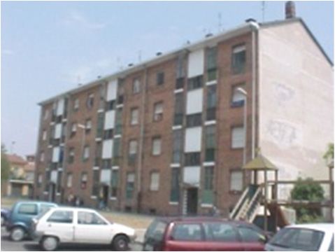
In order to better present this trend, the box plots of thermal energy load for heating in
the month of January and for cooling in the month of August are shown in Figures 4 and 5.
The figures indicate that both for MFH and AB, the mean values for the month of January
are almost the same for all future weather files, while the deviation of F-TMY is lower
than the three other files. On the other hand, for the month of August, the mean values
of WS, MET, and CCW are significantly higher than F-TMY. The reason lies in the fact
(a) that the dynamical downscaled weather data in comparison (b) with the statistical ones better
represents the temporal variability of climate, which leads to a more consistent dataset.
Figure 3. Net thermal energy
Asneeds for heating
another outcome and
ofcooling normalized by
the inconsistency in the
theconditioned floor area for weather
statistical downscaled a mono family
files, both
house (a) and apartment block (b) for IWEC (Present), Weathershift (WS), Meteonorm (MET), CCWorldWeatehr-Gen
figures demonstrate the overestimation of the data in the thermal energy load for cooling
(CCW), and F-TMY. All future weather files are for 2050s considering RCP 8.5.
in August.
(a) (b)
Figure 4. Boxplots of heating loads in January (a) and cooling loads in August (b) of the mono family house for IWEC
(Present), Weathershift (WS), Meteonorm (MET), CCWorldWeatehr-Gen (CCW), and F-TMY. All future weather files are
for 2050s considering RCP 8.5.
(a) (b)
Figure 4. Boxplots
Boxplots of
of heating
heating loads
loads in
in January
January (a) and cooling loads in August (b) of the mono family house for IWEC
(Present), Weathershift (WS), Meteonorm (MET),CCWorldWeatehr-Gen
(Present), Weathershift (WS), Meteonorm (MET), CCWorldWeatehr-Gen (CCW),
(CCW), and
and F-TMY.
F-TMY. AllAll future
future weather
weather filesfiles
are are
for
for 2050s considering RCP
2050s considering RCP 8.5. 8.5.
The adaptive comfort analysis in free floating condition, of MFH and AB for IWEC
(Present), Weathershift (WS), Meteonorm (MET), CCWorldWeatehrGen (CCW), and F-TMY
is presented in Figure 6. The graphs show the distribution of hours of the cooling period
(April 16th until October 14th: 4368 hours) in three ranges: comfort, warm discomfort, and
cold discomfort. The discrepancy between F-TMY and other future weather data is pointed
out. The percentage of warm discomfort hours for the WS, MET, and CCW is almost the
same and equals around 40% for MFH and 90% for AB. For the F-TMY, the percentage
of warm discomfort hours is less for both cases (29% for MFH and 72% for AB). This
discrepancy can be found in Figure 7 where boxplots of last floor operative temperature of
MFH (a) and AB (b) in August for present and different future weather data are presented.Climate 2021, 9, 37 11 of 16
In this case, despite having similar dispersions, the mean values of last floor operative
temperature of F-TMY is significantly lower than the mean value of the other three future
(a) weather datasets for both MFH and AB. This is strongly dependent (b) on the lower dispersion
of temperature values for F-TMY. If we now turn to the comparison of the two building
Figure 5. Boxplots of heatingtypes,loads in January (a)inand
occupants ABcooling load in August
will experience (b) of the apartment
overheating much more block for IWEC
often (Present),
than the occupants
Weathershift (WS), Meteonorm (MET), CCWorldWeatehr-Gen (CCW), and F-TMY. All future weather files are for 2050s
in MFH because of a reduced potentiality of exploiting the heat transfer in AB through
considering RCP 8.5.
the envelope for ejecting heat produced by internal and solar sources. This is due to the
lower S/V value and larger window-to-wall ratio (WWR) of the AB compared to MFH.
The adaptive comfort analysis in free floating condition, of MFH and AB for IWEC
In addition, hours of exceedance (HE) for all the weather datasets for MFH and AB are
(Present), Weathershift (WS), Meteonorm (MET), CCWorldWeatehrGen (CCW), and F-
Climate 2021, 9, 37 presented in Table 1. It is observed that the absolute change of the increase in the HE 11 for
of 16
TMY is presented in Figure 6. The graphs show the distribution of hours of the cooling
statistically downscaled future weather datasets is almost the same, while for dynamically
period (April 16 until October 14 : 4368 hours) in three ranges: comfort, warm discom-
th th
downscaled future weather, data are significantly lower.
fort, and cold discomfort. The discrepancy between F-TMY and other future weather data
is pointed out. The percentage of warm discomfort hours for the WS, MET, and CCW is
almost the same and equals around 40% for MFH and 90% for AB. For the F-TMY, the
percentage of warm discomfort hours is less for both cases (29% for MFH and 72% for
AB). This discrepancy can be found in Figure 7 where boxplots of last floor operative tem-
perature of MFH (a) and AB (b) in August for present and different future weather data
are presented. In this case, despite having similar dispersions, the mean values of last floor
operative temperature of F-TMY is significantly lower than the mean value of the other
three future weather datasets for both MFH and AB. This is strongly dependent on the
lower dispersion of temperature values for F-TMY. If we now turn to the comparison of
the two building types, occupants in AB will experience overheating much more often
than the occupants in MFH because of a reduced potentiality of exploiting the heat trans-
(a)fer in AB through the envelope for ejecting heat produced (b)by internal and solar sources.
This is due to the lower S/V value and larger window-to-wall ratio (WWR) of the AB com-
Figure5.5.Boxplots
Figure Boxplotsofofheating
heating loads
loads
pared ininMFH.
to January
JanuaryIn(a)(a) andcooling
and cooling
addition, load
load
hours ofinin August(b)
August
exceedance (b)ofof theapartment
the
(HE) apartment
for block
all theblock
weather forIWEC
for IWEC (Present),
(Present),
datasets for MFH
Weathershift (WS), Meteonorm
Weathershift (WS), Meteonorm (MET), CCWorldWeatehr-Gen (CCW), and F-TMY. All future weather files are for2050s
2050s
and (MET),
AB areCCWorldWeatehr-Gen
presented in Table 1.(CCW), and F-TMY.
It is observed that All
thefuture
absolute weather
change filesof
are for
the increase in
considering RCP
considering RCP 8.5. 8.5.
the HE for statistically downscaled future weather datasets is almost the same, while for
dynamically downscaled future weather, data are significantly lower.
The adaptive comfort analysis in free floating condition, of MFH and AB for IWEC
(Present), Weathershift (WS), Meteonorm (MET), CCWorldWeatehrGen (CCW), and F-
TMY is presented in Figure 6. The graphs show the distribution of hours of the cooling
period (April 16th until October 14th: 4368 hours) in three ranges: comfort, warm discom-
fort, and cold discomfort. The discrepancy between F-TMY and other future weather data
is pointed out. The percentage of warm discomfort hours for the WS, MET, and CCW is
almost the same and equals around 40% for MFH and 90% for AB. For the F-TMY, the
percentage of warm discomfort hours is less for both cases (29% for MFH and 72% for
AB). This discrepancy can be found in Figure 7 where boxplots of last floor operative tem-
perature of MFH (a) and AB (b) in August for present and different future weather data
are presented. In this case, despite having similar dispersions, the mean values of last floor
operative temperature of F-TMY is significantly lower than the mean value of the other
three future weather datasets for both MFH and AB. This
(a) (b) is strongly dependent on the
lower dispersion of temperature values for F-TMY. If we now turn to the comparison of
Figure
Figure 6.
6. Adaptive
Adaptive comfort
comfort analysis
analysis for aamono
monofamily
forbuilding family house (a)
(a)and
andapartment block (b)(b)for
forIWEC (Present),
(Present),Weathershift
the two types,house
occupants apartment
in AB willblockexperience IWEC
overheating Weathershift
much more often
(WS),
(WS), Meteonorm
Meteonorm (MET),
(MET), CCWorldWeatehr-Gen
CCWorldWeatehr-Gen (CCW),
(CCW), and
and F-TMY.
F-TMY. All
All future
future weather
weather files
files are
are for 2050s
for 2050s considering
considering
RCP 8.5.
than the occupants in MFH because of a reduced potentiality of exploiting the heat trans-
RCP 8.5. fer in AB through the envelope for ejecting heat produced by internal and solar sources.
This is due to the lower S/V value and larger window-to-wall ratio (WWR) of the AB com-
pared to MFH. In addition, hours of exceedance (HE) for all the weather datasets for MFH
and AB are presented in Table 1. It is observed that the absolute change of the increase in
the HE for statistically downscaled future weather datasets is almost the same, while for
dynamically downscaled future weather, data are significantly lower.Climate 2021,
Climate 2021, 9,
9, 37
37 12 of
12 of 16
16
(a) (b)
Figure 7.
Figure 7. Boxplot
Boxplot of
of last
last floor
floor operative
operative temperature
temperature of
of aa mono
mono family
family house
house (a)
(a) and
and apartment
apartment block
block (b)
(b) in
in August,
August, for
for
IWEC (Present), Weathershift (WS), Meteonorm (MET), CCWorldWeatehr-Gen (CCW), and F-TMY. All future
IWEC (Present), Weathershift (WS), Meteonorm (MET), CCWorldWeatehr-Gen (CCW), and F-TMY. All future weather files weather
filesfor
are are2050s
for 2050s considering
considering RCP 8.5.
RCP 8.5.
Table 1. Electrical energy demandIn addition,
per Table
unit of area and 1hours
also of
summarizes theavalues
exceedance for of thehouse
mono family electrical
(MFH) energy demand per
and apartment
unit of area (E el/Af). The Eel/Af increases in MFH and AB similarly for WS, MET, and CCW,
block (AB), for IWEC (Present), Weathershift (WS), Meteonorm (MET), CCWorldWeatehr-Gen (CCW), and F-TMY. All
whileconsidering
future weather files are for 2050s the absoluteRCPchange
8.5. is not significantly high. On the other hand, Eel/Af slightly de-
creases for F-TMY in both cases. The reason can be explained below: as mentioned before,
a future valueWS for the mean seasonal
METefficiency of the CCW heating (ƞH,g) and theTMY-R
cooling (ƞC,g)
IWEC
generation subsystem was
Absolute adopted to consider
Absolute the increase of ambient
Absolute temperature
Absolute due
climate change. The mean
Change seasonal efficiency
Change increases for the
Change heating and decreases
changefor
Eel /Af the cooling for all the future weather datasets. However, due to the lower discrepancy of
38.7 40.7
the temperature 2 for F-TMY
values 2.8
41.5 compared 1.8
40.5 future weather
to other −8.9
29.8 the increase
datasets,
SFH [kWh m−2 ]
HE[h] for ƞH,g in887
222 the dynamical
665 downscaled
877 model
655 is more, 910while the688decreases638in the ƞC,g416
is less.
Eel /Af Consequently, according to Equation (4), the reduction in the energy for winter condition-
22.9 29 6.1 29.5 6.6
case of 28.1 5.2
if the19.4 −3.5
AB [kWh m−2 ] ing outweighs the cooling demand in the F-TMY. Finally, variation of Eel/Af
HE[h] 1273 1995 722 2060 787 1984 711
for MFH and AB are compared, the absolute changes are lower for MFH, which comes 1596 323
from its higher S/V value that skews the energy usage of it more toward the heating re-
gime.In addition, Table 1 also summarizes the values of the electrical energy demand per
unit of area (Eel /Af ). The Eel /Af increases in MFH and AB similarly for WS, MET, and
Table 1. Electrical energy demand per unit of area and hours of exceedance for a mono family house (MFH) and apartment
CCW, while the absolute change is not significantly high. On the other hand, Eel /Af slightly
block (AB), for IWEC (Present), Weathershift (WS), Meteonorm (MET), CCWorldWeatehr-Gen (CCW), and F-TMY. All
decreases for F-TMY in both cases. The reason can be explained below: as mentioned
future weather files are for 2050s considering RCP 8.5.
before, a future value for the mean seasonal efficiency of the heating (η H,g ) and the cooling
(η C,g ) generation
WS subsystem was adoptedMET to consider the increase of ambient
CCW temperature
TMY-R
IWEC due climate change. AbsoluteThe mean seasonal efficiency
Absolute increases for the
Absolute heating and decreases
Absolute
for the cooling for all
change the future weather datasets.
change However, due
change to the lower discrepancy
change
of the temperature values for F-TMY compared to other future weather datasets, the
Eel/Af
38.7increase 40.7for η H,g in
2 the dynamical
41.5 2.8
downscaled 40.5 1.8 while
model is more, 29.8 −8.9 in
the decreases
SFH [kWh m-2 ]
the η C,g is less. Consequently, according to Equation (4), the reduction in the energy for
HE[h] 222winter887 conditioning665 outweighs 877 the cooling
655 demand 910 in the 688 638 Finally,
case of F-TMY. 416if the
Eel/Af
22.9variation 29 of Eel /A6.1
f for MFH 29.5
and AB are 6.6
compared,28.1the absolute
5.2changes 19.4
are lower for
-3.5MFH,
AB [kWh m-2 ] which comes from its higher S/V value that skews the energy usage of it more toward
HE[h] 1273the heating
1995 regime. 722 2060 787 1984 711 1596 323
5. Conclusions
5. Conclusions
Statistical
Statistical and
anddynamical
dynamicalarearetwo
twomain
mainapproaches
approachestotodownscale
downscaleglobal climate
global models
climate mod-
for creating weather datasets to be used in building energy simulation. Considering
els for creating weather datasets to be used in building energy simulation. Considering
there
there are
are different
different methodologies
methodologies that
that use
use these
these approaches,
approaches, evaluating
evaluating their
their suitability
suitability
and
and robustness is vital. This study set out to compare WeatherShift, Meteonorm, and
robustness is vital. This study set out to compare WeatherShift, Meteonorm, and
CCWorldWeatherGen—which are common weather generator tools applying statistical
CCWorldWeatherGen—which are common weather generator tools applying statistical
downscaling—in addition to a TMY created using a high-quality regional climate models
downscaling—in addition to a TMY created using a high-quality regional climate modelsClimate 2021, 9, 37 13 of 16
database (from Euro-CORDEX) that applies the dynamical downscaling. All future weather
files are for the 2050s considering RCP 8.5. Two representative buildings of the Italian
residential building stock, including a mono family house (MFH) and an apartment block
(AB), were selected to perform the analysis.
The results of this investigation show that different statistical downscaled future
weather datasets created by weather generators predict the future energy performance and
comfort analysis of the buildings quite similarly, compared to the dynamical one. This
is demonstrated by almost the same values in the mean outdoor dry-bulb temperature,
relative changes of thermal energy need for heating and cooling normalized by the condi-
tioned floor area, mean value of thermal energy load for heating and cooling, the hours
of discomfort, and the absolute changes in the electrical energy demand per unit of area.
However, when it comes to the dynamical downscaled weather data, the above-mentioned
parameters follow a different pattern. As an example, while the discomfort hours per-
centage for the WS, MET, and CCW equals around 40% for MFH and 90% for AB, for the
F-TMY, this percentage is 29% for MFH and 72% for AB. Consequently, it was verified that
dynamical downscaling, by better representing the spatial and temporal variability of local
climate, provides physically consistent datasets.
The other significant result of this study is reached by comparing different building
types. In more detail, the observed discrepancy between the future predictions of statistical
and dynamical downscaling is affected not only by using different approaches for creating
future weather datasets but also by building type. As an example, the thermal energy
need for cooling in MFH for statistical downscaled datasets increases around 170%, and
for the dynamical one, it increases around 70%. On the other hand, in AB, this parameter
increases 100% for statistical downscaled data and around 40% for the dynamical one. This
inequality in relative variation comes from the different magnitude of the present energy
need for different building types. For buildings with a higher shape factor (MFH), the
heating energy demand dominates the cooling energy demand, which also make them
more sensitive to the climate change.
Overall, this study has provided a deeper insight into analyzing the effect of climate
change on the future energy performance of buildings by considering different future
weather datasets and building types. Firstly, it was shown that the climate change impact
magnitude is not equal for different case studies, so that in a changing climate, performing
a regional and localized analysis becomes vital. In addition, the results demonstrated that
morphing method—regardless of its way of application—can provide adequate information
to perform comparative analysis on long-term changes in energy building performance.
However, the existing inconsistency within this method may lead to high prediction errors.
In this case, the dynamical downscaling method is found to be more reliable when the aim
is to develop, assess, and communicate resilient solutions to withstand as well as prevent
the future impacts of climate change on building energy performance. Further studies
are suggested to be carried out to consider model uncertainties of RCMs by following an
ensemble-based approach. In addition, it is important to bear in mind that RCMs have
been run not only for future but also for historical period. So, they can be compared with
the real data, and the biases associated with the climate model data can be adjusted to
reduce uncertainties and increase their physical consistency. This possibility does not exist
for statistical downscaling method tools, as they are based on transforming the actual real
data; it is possible to say they are often “black-box” tools.
Author Contributions: Conceptualization, M.P. and V.C.; methodology, I.B., M.P, M.Z., and V.C.;
software, M.P.; formal analysis, M.P.; investigation, M.P. and M.Z.; resources, M.P. and M.Z.; data
curation, I.B. and M.P.; writing—original draft preparation, M.P.; writing—review and editing, I.B.,
M.Z., and V.C.; visualization, M.P.; supervision, V.C.; project administration, M.Z. and V.C. All
authors have read and agreed to the published version of the manuscript.
Funding: This research received no external funding.You can also read