Electric Vehicle Routing with Charging/Discharging under Time-Variant Electricity Prices
←
→
Page content transcription
If your browser does not render page correctly, please read the page content below

Electric Vehicle Routing with Charging/Discharging
                                                    under Time-Variant Electricity Prices
                                                                                                    Bo Lin
                                                                   University of Toronto, 5 King’s College Rd, Toronto, ON M5S 3G8, Canada
arXiv:2012.09357v4 [math.OC] 10 Jun 2021

                                                                                              blin@mie.utoronto.ca

                                                                                              Bissan Ghaddar
                                                     Ivey Business School, University of Western Ontario, 1255 Western Road, London, ON N6G 0N1, Canada
                                                                                              bghaddar@uwaterloo.ca

                                                                                              Jatin Nathwani
                                                               University of Waterloo, 200 University Avenue W., Waterloo, ON N2L 3G1, Canada
                                                                                            nathwani@uwaterloo.ca

                                                The integration of electric vehicles (EVs) with the energy grid has become an important area of research due
                                                to the increasing EV penetration in today’s transportation systems. Under appropriate management of EV
                                                charging and discharging, the grid can currently satisfy the energy requirements of a considerable number
                                                of EVs. Furthermore, EVs can help enhance the reliability and stability of the energy grid through ancillary
                                                services such as energy storage. This paper proposes the EV routing problem with time windows under
                                                time-variant electricity prices (EVRPTW-TP) which optimizes the routing of an EV fleet that are delivering
                                                products to customers, jointly with the scheduling of the charging and discharging of the EVs from/to the
                                                grid. The proposed model is a multiperiod vehicle routing problem where EVs can stop at charging stations
                                                to either recharge their batteries or inject stored energy to the grid. Given the energy costs that vary based on
                                                time-of-use, the charging and discharging schedules of the EVs are optimized to benefit from the capability
                                                of storing energy by shifting energy demands from peak hours to off-peak hours when the energy price is
                                                lower. The vehicles can recover the energy costs and potentially realize profits by injecting energy back
                                                to the grid at high price periods. EVRPTW-TP is formulated as an optimization problem. A Lagrangian
                                                relaxation approach and a hybrid variable neighborhood search/tabu search heuristic are proposed to obtain
                                                high quality lower bounds and feasible solutions, respectively. Numerical experiments on instances from the
                                                literature are provided. The proposed heuristic is also evaluated on a case study of an EV fleet providing
                                                grocery delivery at the region of Kitchener-Waterloo in Ontario, Canada. Insights on the impacts of energy
                                                pricing, service time slots, range reduction in winter as well as fleet size are presented.

                                                Key words : Electric vehicle routing; energy storage; sustainable last-mile delivery; mixed integer
                                                  programming; Lagrangian relaxation, metaheuristics.

                                           1.     Introduction
                                           Over the recent years, sustainability has become a paramount global concern. In the transportation
                                           sector, public and private institutions are attempting to increase the penetration of electric vehicles

                                                                                                       1
2

(EVs) due to their ability to mitigate greenhouse gas emission and their direct impact on reducing
particulate matter pollution (Boulanger et al. 2011, Waraich et al. 2013). Companies are also
investigating the use of new green technologies due the potential brand benefits given the growing
demands for green products (Kleindorfer et al. 2005, Dekker et al. 2012). UPS, FedEx, and Walmart
are among the leading companies that have deployed EV fleets in their operations (Winston 2018).
As a consequence, the past decade has seen a rapid expansion of EV adoption (Hertzke et al. 2019).
According to Statistics Canada (2019), the number of new EV registrations has increased from
25,163 in 2014 to 69,010 in 2018. As projected by Canada Energy Board (National Energy Board
2018), EVs will account for over 60% of the new motor vehicle registrations in Canada by 2040.
    Not surprisingly, the growing penetration of EVs has a significant impact on the power system.
Previous studies have shown that, without proper management, the EVs will represent a sizable
fraction of the total demand for energy (Triviño-Cabrera et al. 2019, Dyke et al. 2010). As a result,
the gap between peak and off-peak demands will increase, and the ramp requirements will affect the
stability and reliability of the power network (Villar et al. 2012). With optimized scheduling of the
charging, the existing power system infrastructure can accommodate the energy requirements of
a considerable number of EVs (Razeghi and Samuelsen 2016, Kintner-Meyer et al. 2007, Letendre
et al. 2008). In doing so, the need for installing new capacity, which is expensive, time-consuming,
and harmful to the environment, can be minimized (Villar et al. 2012). Furthermore, EVs can be
incorporated into the power grid as a reliable and cost-effective distributed power storage (Kempton
and Letendre 1997). By optimizing the charging and discharging to the grid, an EV fleet connected
to the energy grid can assist to level out peaks in the overall electricity consumption and support
the utilization of intermittent renewable energy.
    Although the vehicle-to-grid (V2G) connectivity represents an enticing idea, it nonetheless
remains in the pilot stages of development (Sovacool et al. 2018), and is mainly focused around a
centralized architecture where a controller manages the ancillary services of a large group of EVs
that are charging and discharging energy from/to the grid (Guille and Gross 2009, Sortomme and
El-Sharkawi 2010). Commercial EV fleet owners such as logistics and e-commerce companies are
naturally strong candidates for realizing the benefits of EV integration in the energy grid as they
aggregate a large number of EVs.
    This paper considers a delivery service system that operates a fleet of EVs that are primarily used
to deliver products to customers. The EVs can be charged or discharged at the home depot or at
charging stations in the network. When charging, a cost is paid according to the energy price at the
time of use. If energy is discharged to the grid, a profit is creditted to the EV. We thus propose the
EV routing problem with time windows under time-variant electricity prices (EVRPTW-TP) which
optimizes the monetary cost of the EV fleet operation while allowing the charging and discharging
3

of EVs at time-of-use electricity prices. EVRPTW-TP extends the EV routing problem with time
windows (Schneider et al. 2014) by incorporating additional operational constraints, allowing the
partial charging and discharging of the EVs, and accounting for the time-varying electricity prices.
In order to solve EVRPTW-TP, a hybrid Variable Neighborhood Search/Tabu Search (VNS/TS)
heuristic that can generate high quality feasible solutions efficiently is developed. A Lagrangian
Relaxation that is solved by a cutting plane approach is also proposed to obtain lower bounds.
The results are evaluated using a variation of the widely-used vehicle routing instances of Solomon
(1987). Finally, the model is evaluated using a case study of an EV fleet performing grocery delivery
in the Kitchener-Waterloo region in Ontario, Canada. Managerial insights are drawn with respect
to electricity pricing, time slots design, winter range reduction, and fleet size.
  This paper is the first to investigate the joint optimization of routing and charge/discharge
scheduling of multiple EVs under time-variant electricity prices. The proposed model provides
operational decisions to support commercial EV fleet operators in order to lower the overall energy
costs. The proposed model also offers important implications for policy makers and can assist the
power system regulators to better understand the impact of EV fleets on energy markets, and to
predict and estimate the market reaction to energy price adjustments. The managerial insights
extracted can help policy makers in creating more efficient energy pricing schemes to maximize the
environmental and economic benefits from the widespread adoption of commercial EV fleets.
  The rest of this paper is organized as follows. Following this introductory section, Section 2
reviews the related literature. The proposed problem is formulated in Section 3. The Lagrangian
relaxation is presented in Section 4 and the proposed VNS/TS heuristic is then discussed in Sec-
tion 5. Computational results and the case study are presented in Sections 6 and 7, respectively.
Finally, Section 8 concludes and highlights future research directions.

2.   Literature Review
The vehicle routing problem (VRP) was first proposed by Dantzig and Ramser (1959) as a gener-
alization of the well-known travelling salesman problem. In general, given a set of geographically
scattered customers each associated with a demand, the VRP seeks to assign customers to vehicles
in such a manner that the demand of each customer is satisfied while the total distance travelled
by the fleet of vehicles to serve all the customers is minimized.
  Since the introduction of the classical VRP, numerous variants were developed and investigated
to account for realistic constraints and objectives. One of the most common variants is the VRP
with time windows where visits to individual customers are restricted to fixed time intervals (Russell
1977). Another variation is the green vehicle routing problem introduced by Erdoğan and Miller-
Hooks (2012) which particularly models alternative fuel vehicles and accounts for the opportunity to
4

extend a vehicle’s distance limitation by visiting an en-route station facility to replenish. Schneider
et al. (2014) tailors this framework specifically to EVs and proposes the EV routing problem with
time windows (EVRPTW). Instead of using a constant replenishment time as in Erdoğan and
Miller-Hooks (2012), EVRPTW assumes a linear energy charging time that is associated with the
battery level of the electric vehicle upon arrival to a station.
    Following Erdoğan and Miller-Hooks (2012) and Schneider et al. (2014), various studies have
investigated the optimization of EV routing and charging/discharging operations which are sum-
marized in Table 1. In the uni-directional V2G contexts, Felipe et al. (2014) and Keskin and Çatay
(2016) consider partial charging strategies with multiple types of chargers, each with a different
charging speed and static unit cost. Yang et al. (2015) optimize over the monetary cost of an EV
providing pickup and delivery services under time-variant charging prices. The problem is extended
by Barco et al. (2017) to a multi-vehicle case incorporating the battery degradation cost. Also under
time-variant electricity prices, Yu and Lam (2018) models a fleet of autonomous EVs that pro-
vide customer delivery and renewable energy storage to the energy grid. A quadraticly-constrained
mixed integer program is formulated and three objective functions are proposed to either minimize
the total driving distance, to maximize the amount of energy charged from renewable sources, or
to minimize the amount of time until the vehicles reach the final destinations.
    In the bi-directional V2G contexts where EVs are allowed to inject energy back to the grid, Tang
et al. (2017) consider a set of EVs travelling from their origins to the corresponding destinations
without en-route customers. EVs can detour for en-route charging and discharging to two types of
stations, one providing renewable energy at a low price while the other is a normal station with
higher charging cost and provide discharging reward. The energy prices do not vary across time,
the objective is to minimize the overall monetary cost of the EV fleet. Triviño-Cabrera et al. (2019)
extend the problem by incorporating intermediate stops for EVs and considering time-variant
electricity prices as well as battery degradation cost. However, the model is not able to coordinate
the schedules for different EVs and does not have a customer delivery component. Abdulaal et al.
(2017) study a similar problem for an EV fleet considering EV congestion at charging/discharging
stations. The customer assignments to different EVs are assumed to be given, the problem thus de-
generate to a single EV case. Moreover, the routing and charging decisions are made sequentially,
which are likely to be sub-optimal. To the best of our knowledge, no previous research has been
conducted to jointly optimize the routing and charging/discharging operations of multiple EVs
under time-variant electricity prices.
    The model proposed in this paper fills the gap between considering energy networks and trans-
portation independently. The proposed model extends the work of Schneider et al. (2014) to include
energy discharging to the grid in a multi-period framework that also accounts for the changing
5
energy prices. Thus the proposed model can be seen as a bi-directional V2G system where the fleet
of EVs whose primary purpose is to deliver products to customers can also be used to store and
redistribute energy from/to the energy grid. The EV routing problem with time windows under
time-variant electricity prices is presented next.
Table 1 Existing literature about optimization of EV routing and charging/discharging operations
Customer Delivery Charging Discharging Time-Variant Prices Multi-EVs
Schneider et al. (2014) X full X
Felipe et al. (2014) X partial X
Yang et al. (2015) X partial X
Keskin and Çatay (2016) X partial X
Desaulniers et al. (2016) X partial X
Tang et al. (2017) partial X X
Abdulaal et al. (2017) X partial X X
Barco et al. (2017) X partial X X
Yu and Lam (2018) X partial X
Triviño-Cabrera et al. (2019) partial X X
EVRPTW-TP X partial X X X
3. EV Routing under Time-Variant Electricity Prices
3.1. Framework and Assumptions
To formulate EVRPTW-TP, a complete directed graph G(Vc,s,od , E) is considered where Vc,s,od
denotes the set of all nodes and E is the set of all edges. The nodes are partitioned into three
distinct categories: customer nodes, station nodes, and a depot. Let Vc = {1, 2, . . . , N } denote the
set of N customers where each node i is associated with a demand qi , a service time si , and a time
window [ei , li ] during which an EV should arrive to node i. Let Vs = {N + 1, . . . , N + S } be the set
of S en-route stations where an EV can charge or discharge energy. The depot is denoted by two
nodes 0 and N + S + 1, i.e. Vod = {0, N + S + 1}, where node 0 is the start of the vehicle route and
N + S + 1 is the end of the route. Each station or depot node i ∈ Vs ∪ Vod has a time window [ei , li ]
from the start to the end of the planning horizon. Each edge (i, j) is associated with a distance aij
and time tij that denotes the travel distance and time between nodes i and j, respectively.
An EV’s instantaneous power depends on its mass, acceleration, as well as aerodynamic, rolling,
and grade resistances (Wu et al. 2015). The change in EV mass is negligible for certain applica-
tions, e.g. small-package delivery, while the resistances could be captured by the driving speed and
acceleration assuming related parameters that are given in (Schneider et al. 2014). Additionally,
the power consumption does not directly translate to the battery’s state of charge due to the non-
linear battery efficiency and other real-world characteristics such as temperature (Hannan et al.
2017). Incorporating these realistic features could more accurately describe the energy consump-
tion and recharging/discharging processes, yet they will introduce computational burdens. For the
sake of keeping the model tractable, following Schneider et al. (2014) and Desaulniers et al. (2016),6
1
we assume a constant energy consumption rate g and a constant charging speed α
. The energy
consumption for edge (i, j) is thus given by cij = gaij , the time required to recharge the energy
consumed by traveling along edge (i, j) is given by fij = αcij .
We assume a commercial EV fleet consisting of K homogeneous EVs, each with a load capacity
Q and a battery capacity C. The time required to fully recharge the battery from 0 is defined as
B = αC. At the beginning of the planning horizon, all the EVs are at the depot (node 0) with a full
battery. All EVs should return to the depot (node N +S +1) before the end of the planning horizon.
During each visit to a station or to the depot, an EV can either pay to charge its battery or make
profits by injecting energy back to the grid from its battery. The charging cost and discharging
reward vary according to the time period (time-of-use energy pricing). We assume that EVs are
allowed to perform either charging or discharging during their station visits, but are not allowed
to perform both during the same time period.
The planning horizon is formed of |T | consecutive discrete periods, each of length δ. Each time
period t refers to a time interval [δ(t − 1), δt) and is associated with a buying (from the grid)
energy price ptb and a selling (to the grid) energy price pts . We assume that if an EV is to charge or
discharge during a time period, then it has to do so for the full time period. Due to the constant
δ
linear charging/discharging assumption, a fixed amount of energy B
C would be charged/discharged
t
during each period, we therefore can calculate a charging cost Pre = Bδ Cptb and a discharging reward
t
Pdis = Bδ Cpts for each period. EVs are recharged back to full battery capacity during the night using
pnight
at a lower energy price pnight . For the ease of presentation, we define Pnight = α
as the cost of
charging per unit of time during the night. The notations are summarized in Table 2.
The problem formulation that is proposed next jointly optimizes the routes and charg-
ing/discharging schedule of the K vehicles by minimizing the net electricity cost given that all
customer demands are satisfied.
3.2. Problem Formulation
To formulate EVRPTW-TP, the following binary variables are introduced:
(
1 if edge (i, j) is traveled by vehicle k,
xijk =
0 otherwise,
(
1 if vehicle k charges its battery at node i at time period t,
ritk =
0 otherwise,
(
1 if vehicle k discharges its battery at node i at time period t,
ditk =
0 otherwise.
The continuous variables are
τik : arrival time of vehicle k at node i,7
Table 2 Summary of the Notation
Definition
Vc Set of customer nodes Vc = {1, 2, . . . , N }
Vs Set of station nodes Vs = {N + 1, . . . , N + S }
Vod Set of depot nodes Vod = {0, N + S + 1}
Vc,s Vc,s = Vc ∪ Vs
Vc,s,o Vc,s,o = Vc ∪ Vs ∪ {0}
Vc,s,d Vc,s,d = Vc ∪ Vs ∪ {N + S + 1}
Vs,d Vs,d = Vs ∪ {N + S + 1}
Vs,o Vs,o = Vs ∪ {0}
Vs,od Vs,od = Vs ∪ Vod
Vc,od Vc,od = Vc ∪ Vod
Vc,s,od Vc,s,od = Vc ∪ Vs ∪ Vod
p Depot node p = N + S + 1
E Set of all edges
T Set of charging/discharging periods
N Number of customers
S Number of stations
K Number of EVs
δ Length of each charging/discharging period
Q Cargo capacity
C Battery capacity
B Amount of time required to fully charge the EV battery from empty
α The reciprocal of the constant charging speed
g Energy consumption rate with respect to distance traveled
aij Travel distance of edge (i, j)
tij Travel time of edge (i, j)
cij Energy consumption along edge (i, j)
fij The amount of time required to charge the energy consumed along edge (i, j)
ei Earliest service start time at node i
li Latest service start time at node i
si Required service time at node i
qi The demand at node i
pnight Unit electricity buying (from the grid) price at night (¢/kWh)
ptb Unit electricity buying (from the grid) price during period t (¢/kWh)
pts Unit electricity selling (to the grid) price during period t (¢/kWh)
Pnight The cost of charging per unit of time at night
t
Pre Cost of charging during period t
t
Pdis Reward for discharging during period t
bik : remaining energy (in terms of charging time) in vehicle k upon arrival to node i,
uik : remaining cargo in vehicle k upon arrival to node i.
The decision variables ritk and ditk are only associated with the station and depot nodes, while the
remaining variables are associated with all the nodes. EVRPTW-TP is formulated as8
K
X X X K
X X
t t
min [ritk Pre − ditk Pdis ]+ Pnight [B − bpk − δ(rptk − dptk )], (1)
k=1 i∈Vs,od t∈T k=1 t∈T
K
X X
s.t. xijk = 1, ∀i ∈ Vc , (2)
k=1 j∈Vc,s,d
X
xipk = 1, ∀k ∈ {1, 2, . . . , K }, (3)
i∈Vc,s,o
X X
xjik − xijk = 0, ∀i ∈ Vc,s , k ∈ {1, 2, . . . , K }, (4)
j∈Vc,s,o j∈Vc,s,d
τik + (tij + si )xijk − δ |T |(1 − xijk ) ≤ τjk , ∀i ∈ Vc,s,o , j ∈ Vc,s,d , k ∈ {1, 2, . . . , K }, (5)
tδ(ritk + ditk ) + tij xijk − δ |T |(1 − xijk ) ≤ τjk , ∀i ∈ Vs,o , j ∈ Vc,s,d , t ∈ T, k ∈ {1, 2, . . . , K }, (6)
ei ≤ τik ≤ li , ∀i ∈ Vc,s,od , k ∈ {1, 2, . . . , K }, (7)
b0k = B, ∀k ∈ {1, 2, . . . , K }, (8)
bjk ≤ bik − fij xijk + B(1 − xijk ), ∀i ∈ Vc , j ∈ Vc,s,d , k ∈ {1, 2, . . . , K }, (9)
X X
bjk ≤ bik + δritk − δditk − fij xijk + B(1 − xijk ), ∀i ∈ Vs,o , j ∈ Vc,s,d , k ∈ {1, 2, . . . , K },
t∈T t∈T
(10)
X
δritk ≤ B − bik , ∀i ∈ Vs,od , k ∈ {1, 2, . . . , K }, (11)
t∈T
X
δditk ≤ bik , ∀i ∈ Vs,od , k ∈ {1, 2, . . . , K }, (12)
t∈T
ritk + ditk ≤ 1, ∀i ∈ Vs,od , t ∈ T, k ∈ {1, 2, . . . , K }, (13)
τik − (t − 1)δ ≤ δ |T |(1 − ditk − ritk ), ∀i ∈ Vs,d , t ∈ T, k ∈ {1, 2, . . . , K }, (14)
ujk ≤ uik − qi xijk + Q(1 − xijk ), ∀i ∈ Vc,s,o , j ∈ Vc,s,d , k ∈ {1, 2, . . . , K }, (15)
u0k = Q, k ∈ {1, 2, . . . , K }, (16)
X
0 ≤ bjk ≤ B xijk , ∀j ∈ Vs , k ∈ {1, 2, . . . , K }, (17)
i∈Vc,s,o
uik , τik ≥ 0, ∀i ∈ Vc,s,od , k ∈ {1, 2, . . . , K }, (18)
xijk ∈ {0, 1}, ∀i ∈ Vc,s,o , ∀j ∈ Vc,s,d , k ∈ {1, 2, . . . , K }, (19)
ritk , ditk ∈ {0, 1}, ∀i ∈ Vc,od , t ∈ T, k ∈ {1, 2, . . . , K }. (20)
The objective function (1) minimizes the net cost, i.e. the total cost of charging the batteries
minus the total reward earned from discharging the batteries. The first part of the objective
function corresponds to the net cost during the planning horizon, while the second part is the cost
of fully recharging back all EVs at night. Constraints (2) ensure that every customer is served
by exactly one EV. Constraints (3) force all the EVs to return to the depot by the end of the9
planning horizon. Constraints (4) guarantee that no route ends at a customer or a station node.
Constraints (5) ensure time feasibility of the edges leaving the customer and the depot nodes,
while constraints (6) deal with the edges originating from charging stations. Constraints (7) ensure
that the time windows of all the nodes are not violated. Constraints (8) indicate that every EV is
fully charged before leaving the depot. Constraints (9)–(10) track the battery capacity along the
route. Constraints (11) indicate that an EV battery cannot be recharged to a level that exceeds its
capacity, while Constraints (12) state that an EV battery cannot be discharged to a level below 0.
Constraints (13) indicate that an EV is allowed to discharge or recharge its battery at a station
or the depot nodes but is not allowed to discharge and recharge during the same time period.
Constraints (14) ensure that an EV cannot start charging/discharging at a station/depot before
arrival and before the start of the time period. Constraints (15) ensure that the demands along a
route are all satisfied, whereas Constraints (16) state that all EVs have a full cargo at the start of
the planning horizon. Constraints (17)–(20) indicate the variables types and limits.
4. Lagrangian Relexation for the EVRPTW-TP
As shown in Section 6.3, solving EVRPTW-TP to optimality is computationally very challenging.
Lagrangian relaxation is a well known algorithm that has been used to address many complex
optimization problems. Particularly, in the context of vehicle routing, Lagrangian relaxation has
been used to address several variants of VRP (Fisher et al. 1997, Kallehauge et al. 2006).
For the EVRPTW-TP, all the constraints other than Constraints (2) are associated with a
particular vehicle k. Given this special structure which is common in vehicle routing problems,
Constraints (2) are relaxed and the violation is penalized in the objective function using the
Lagrangian multipliers λi . The resulting relaxed problem is
K
X X X
t t
ZLR (λ) = min [ritk Pre − ditk Pdis ]
k=1 i∈Vs,od t∈T
K
X X
+ Pnight [B − bpk − δ(rptk − dptk )]
k=1 t∈T
X K
X X
+ λi (1 − xijk ),
i∈Vc k=1 j∈Vc,s,d
s.t. (3) − (20).
Since the EV fleet is homogeneous, problem ZLR (λ) decomposes into K identical sub-problems
X X X
t t
ZSP (λ) = min [rit Pre − dit Pdis ] + Pnight [B − bp − δ(rpt − dpt )]
i∈Vs,od t∈T t∈T
X X
− λi xij ,
i∈Vc j∈Vc,s,d
s.t. (3) − (20).10
The value of the Lagrangian bound ZLR (λ) is
X
ZLR (λ) = K × ZSP (λ) + λi ,
i∈Vc
and the best Lagrangian bound is given by max ZLR (λ). Given H, the set of feasible solutions
λ∈R|Vc |
of the Lagrangian subproblem, the best Lagrangian bound can be found by solving the following
h
problem where rit , dhit , and xhij describe the charging, discharging, and routing schedule associated
with solution h ∈ H, respectively,
X X X X X X
h t
max K × min [rit Pre − dhit Pdis
t
] + Pnight [B − bhp − h
δ(rpt − dhpt )] − λi xhij + λi ,
λ∈R Vc h∈H
i∈Vs,od t∈T t∈T i∈Vc j∈Vc,s,d i∈Vc
which is equivalent to the Lagrangian master problem
X
ZM P = max λi + Kθ,
λ∈RVc
i∈Vc
X X X X X
s.t. θ + λi xhij ≤ h t
[rit Pre − dhit Pdis
t
] + Pnight [B − bhp − h
δ(rpt − dhpt )], ∀h ∈ H.
i∈Vc j∈Vc,s,d i∈Vs,od t∈T t∈T
Since the set H is not known beforehand, we implemented the stablized cutting-plane approach
developed by Kallehauge et al. (2006) to obtain ZM P iteratively starting with an empty set H. The
determination of the set of cutting planes require solution of the subproblem. Given fixed values
of the Lagrangian multipliers λi , the Lagrangian subproblem is solved to obtain ZSP (λ) and a new
feasible solution h ∈ H. The resulting solution generates a cut that is added to the master problem.
The relaxed master problem is solved to obtain new values for the Lagrangian multipliers. The
solution of the relaxed master problem provides an upper bound on the optimal Lagrangian bound
while the optimal solution of ZLR (λ) provides a lower bound. The algorithm iterates until the gap
between the upper and lower bounds is sufficiently small. Alternatively, the Lagrangian bound
can also be obtained by solving the Dantzig-Wolfe reformulation of ZM P using column generation.
Both methods require solving ZSP (λ) repetitively.
The Lagrangian sub-problem has similar structure as the column generation sub-problem intro-
duced by Desaulniers et al. (2016) for EVRPTW. However, it is nontrivial to apply the labeling
algorithm proposed by Desaulniers et al. (2016) to solve ZSP (λ) because of the difference between
their objective functions. Although the EV’s energy consumption along the route is linear with
respect to the total distance, the cost of a unit distance in ZSP (λ) depends on the time of charging
which introduces extra complexity to the problem. In addition, the decision about discharging
is largely independent of the travelling distance and hence we can not formulate the Lagrangian
sub-problem as a elementary shortest path problem with resource constraints. For these reasons,
we use a standard mixed integer programming (MIP) solver to solve ZSP (λ).11
5. VNS/TS Hybrid Heuristic for EVRPTW-TP
The Lagrangian relaxation presented in Section 4 provides lower bounds on the optimal solution
of problem (1)–(20). To obtain upper bounds and very importantly to implement in practice,
good quality feasible solutions are needed relatively quickly. Following the framework presented in
Schneider et al. (2014) for EVRPTW, this section presents a hybrid variable neighborhood search
and tabu search (VNS/TS) meta-heuristic with an annealing mechanism to solve EVRPTW-TP.
Hybrid VNS/TS meta-heuristics have been previously applied successfully for routing problems
(Melechovskỳ et al. 2005, Tarantilis et al. 2008). The overall framework of the VNS/TS is shown in
Algorithm 1. VNS/TS consists of three main components: (1) an initialization step which identifies
an initial solution, (2) a variable neighborhood search (VNS) to diversify the search process from
the current solution, and (3) a tabu search (TS) component that runs for each candidate solution
of VNS for local intensification. VNS/TS stops when the iterations limit is reached or when no
improving solution is identified after a fixed number of consecutive VNS iterations. The details of
each component are presented next.
Algorithm 1 VNS/TS Heuristic For EVRPTW-TP
1: S = initialization()
2: counter ← 0
3: for i = 1, 2, . . . , ηvns do
0
4: S = M ove2N eighbor(S)
5: for j = 1, 2, . . . , ηtabu do
00 0
6: S = T abu(S )
00
7: if fgen (S) > fgen (S ) then
8: counter ← 0
9: else
10: counter ← counter + 1
11: if counter ≥ ηearly then
12: Break
00 00
13: else if Accept(S, S ) then S ← S
5.1. Initialization
In the initialization step, routes are constructed such that each customer with a positive demand is
visited exactly once. For that, the well known sweep heuristic is used to obtain the initial feasible
solution without charging and discharging operations (Cordeau et al. 2001). Customers are first12
sorted according to an increasing order of the geometric angle using as a reference a randomly
selected point. Then, starting from the customer with the smallest angle, customers are inserted to
the active route at the position resulting in the minimal increase of the travel distance of the route.
Once the battery or cargo constraints of the active route are violated, a new route is initiated until
the number of routes used so far is equal to the EV fleet size. Then, all the remaining customers
are inserted into the last route.
5.2. Generalized Cost Function
The VNS/TS meta-heuristic considers infeasible solutions during the search. Similar to Schneider
et al. (2014), a cost function is used to evaluate the quality of a solution S. The generalized cost
function fgen (S) is given by
fgen (S) = felec (S) + βtw Φtw (S) + βbatt Φbatt (S) + βcargo Φcargo (S) (21)
where felec (S) is the net cost of electricity (charging cost minus discharging reward); Φtw (S),
Φbatt (S), and Φcargo (S) are the violations of the time window, battery, and cargo constraints,
respectively; and βtw , βbatt and βcargo are penalty factors corresponding to each violation. The
cumulative net cost felec (S), and the cumulative violations Φtw (S), Φbatt (S), and Φcargo (S) are the
sum of the net costs of the individual routes felec (R) and the individual violations for each route
Φtw (R), Φbatt (R), and Φcargo (R), respectively.
5.2.1. Electricity Cost and Violation Evaluation In order to evaluate the electricity cost
and the violations, let ri denote the ith node along route R of length n. The following metrics are
then defined for every node along a given route
(
0, i = 1
TiE = (22)
E
max min Ti−1 , lri−1 + sri−1 + tri−1 ri , eri , ∀i = 2, 3, . . . , n
L
− tri ri+1 − sri+1 , lri + sri , ∀i = 1, 2, . . . , n − 1
(
min Ti+1
TiL = (23)
|T |δ, i=n
0, i = 0
FS E
TiF S = Ti−1 + max eri − Ti−1 + sri−1 + tri−1 ri , 0 , if ri−1 ∈ Vc (24)
E
max eri − Ti−1 + sri−1 + tri−1 ri , 0 , otherwise
0, i = n
BS
L
TiBS = Ti+1 + max Ti+1 − tri ri+1 − lri − sri , 0 , if ri+1 ∈ Vc (25)
L
max Ti+1 − tri ri+1 − lri − sri , 0 , otherwise13
0, if i = 0
Fi = Fi−1 + fri−1 ri , if ri−1 ∈ Vc (26)
fri−1 ri , otherwise.
TiE is the earliest service start time at node ri without violating any time window constraints
before it. Similarly, TiL is the latest departure time from ri that will not result in any time window
violations after it. TiF S is the forward cumulative slack time, i.e. the difference between earliest
arrival time and the earliest service start time, from the last station/depot to ri . TiBS is the
backward cumulative slack time, i.e. the difference between the latest departure time and the latest
service time, from ri to the preceding station/depot. Fi is the amount of time required to recharge
the energy consumption from the last station/depot to ri .
Cargo Capacity Violation The cargo capacity violation Φcargo (R) of a route R is calculated as
( n )
X
Φcargo (R) = max qri − Q, 0 . (27)
i=1
Time Window Violation We calculate the time window violation for route R as the sum of
violations at each node along R. For the violation at node ri that follows ri−1 with time window
violation, we assume the arrival time at ri−1 is its latest service start time. This assumption is
similar to that of Schneider et al. (2014) to prevent time window violations from propagating along
the route and avoid penalizing a good customer sequence only because it follows a node with time
window violation. The time window violation Φtw (R) for a route R is
n
X
max TiE − lri , 0 .
Φtw (R) = (28)
i=1
Battery Capacity Violation The battery violations Φbatt (R) for a route R is
X
Φbatt (R) = max {Fr − B, 0} . (29)
r∈R∩Vs
5.2.2. Net Electricity Cost To calculate the electricity cost of a given route, a feasible
charging/discharging schedule for each route is computed. Due to the complexity of the problem,
the following assumptions are made to limit the number of potential feasible schedules:
1. The maximum number of station visits is limited to two. In practice, it is likely that this
assumption is reasonable as the EV fleet needs to primarily service customers, and charging activ-
ities are to make sure that the vehicle has enough energy to complete the route and/or to offer
the ancillary service of discharging for additional gain. Furthermore, frequent battery charging and
discharging have a negative impact on the battery health and as such in practice it is expected
that charging and discharging activities are limited to a few station visits.14
2. If a vehicle visits a station to recharge, then the vehicle recharges the battery just enough to
be able to complete the route to reach the depot. This assumption is applicable to the two-station
visit case and excludes the possibility of over-charging at one station to discharge at another station
later.
3. A vehicle is allowed to perform either charging or discharging at stations, but is not allowed
to do both during a single station visit. This assumption reduces the solution space defined by the
MIP formulation.
Given a depot or a station node which is the ith node on route R denoted by ri ∈ R, the time
window during which a vehicle can charge or discharge is TrEi , TrLi . Given that the planning horizon
is discretized,
E thenE the set of time periods during which the vehicle can charge/discharge is given
Tr Tr TrL
by Ti = d δ i e, d δ i e + 1, . . . , b δ i c , namely the connected periods for ri .
Given the ith and the j th node (i < j) of route R where a vehicle can charge/discharge (station
or depot node) and Ti and Tj are the connected periods corresponding to i and j respectively, if a
vehicle charges/discharges at time period t ∈ Ti , then this might make it impossible for the vehicle
to arrive at node j before the start of time period t0 . Thus Mit is defined as the mutually exclusive
set for t ∈ Ti which is the set of all the time periods t0 ∈ Tj where the vehicle cannot reach node j
if it is charging/discharging during time period t. The mutually exclusive set Mit is given by
∅, if δt ≤ TrEi + TrFj S
t
Mi = n 0 o (30)
t : δ(t0 − 1) < TrE + δt − TrE + TrF S , otherwise.
j i j
Given that at most two stations are allowed in each route, three different cases are analyzed
to find a feasible charging/discharging schedule corresponding to the three special cases of zero
stations, one station, and two stations routes, respectively.
Zero stations If there are no stations along the vehicle’s route and given that the EV is fully
charged at the starting depot, then the only potential activities are to discharge the EV at the
starting and/or ending depot. The maximum amount of time periods during which the EV can
discharge while ensuring that there is enough energy available to cover the full route is given by
Ω = b B−F
δ
n
c. Given the connected periods T1 and Tn at the two depot nodes (the first and the last
node along R) and the set of mutually exclusive time periods M1t for each time period t ∈ T1 , the
following mixed integer program maximizes the revenue from energy discharge
X X
Υ∗ = max t
Pdis dt1 + t
Pdis dtn (31)
d
t∈T1 t∈Tn
X X
s.t. dt1 + dtn ≤ Ω, (32)
t∈T1 t∈Tn
dt1 + dkn ≤ 1, ∀t ∈ T1 , ∀k ∈ M1t , (33)
dtj ∈ {0, 1}, ∀j ∈ {1, n}, ∀t ∈ Tj . (34)15
where dm
j is a binary decision variable indicating if the EV discharges at node j during time
period m. We note that by enumerating the end period where the EV discharges at r1 , the MIP
simplifies to |T1 | 0-1 knapsack problems with unit item weights that can be solved very efficiently.
Given the optimal solution d∗ , the net cost of electricity for route R is given by
∗ ∗
X X
felec (R) = −Υ∗ + (Fn + δdt1 + δdkn ) × Pnight . (35)
t∈T1 k∈Tn
One station Given that an EV is visiting a station (k th node along route R), then one possibility
is that the EV has to recharge the battery at the station node to make sure there is enough energy
to reach the end-of-route depot (nth node along route R). This case occurs if ∆ = Fk + Fn − B > 0.
Otherwise, the EV can either discharge energy at the station or recharge in order to discharge later
at the depot. Given the sets of connected time periods T1 , Tk , and Tn , for the 1st , k th , and last
node along route R, respectively, and the mutually exclusive sets M1t for each time period t ∈ T1 ,
and Mkt for each time period t ∈ Tk , the following mixed integer program maximizes the revenue
from energy charging and discharging
X X X X
Υ∗ = max t
Pdis dt1 + t
Pdis dtk + t
Pdis dtn − t t
Pre rk , (36)
d,r
t∈T1 t∈Tk t∈Tn t∈Tk
(
X X X X ≤ b −∆ c if ∆ < 0,
s.t. dt1 + dtk + dtn − rkt ∆
δ
(37)
t∈T1 t∈Tk t∈Tn t∈Tk
=dδ e otherwise,
X X
δ rkt ≤ Fk + δ dt1 , (38)
t∈Tk t∈T1
!
X X X
δ dt1 + dtk + Fk + Fn ≤ B + δ rkt , (39)
t∈T1 t∈Tk t∈Tk
X
dtk ≤ |Tk |y, (40)
t∈Tk
X
rkt ≤ |Tk |(1 − y), (41)
t∈Tk
dt11 + rkt2 + dtk2 ≤ 1, ∀t1 ∈ T1 , ∀t2 ∈ M1t1 , (42)
rkt1 + dtk1 + dtn2 ≤ 1, ∀t1 ∈ Tk , ∀t2 ∈ Mkt1 , (43)
dtj , rjt ∈ {0, 1}, ∀j ∈ {1, k }, ∀t ∈ Tj , (44)
y ∈ {0, 1}. (45)
where dm m
j and rj are binary decision variables indicating if the EV discharges and charges at
node j during time period m, respectively. Constraint (37) specifies the amount of charging and
discharging given different values of ∆. Constraint (38) ensures the EV battery capacity is not
violated after charging/discharging at the en-route station. Constraint (39) guarantee the EV has16
enough energy to complete the trip. Constraints (40)-(41) force that the EV can perform either
charging or discharging at the station. Constraints (42)-(43) describe the mutual exclusiveness
among periods at r1 , rk and rn . Constraint (44)-(45) specify the domains of the decision variables.
Given the optimal solution d∗ and r∗ , the net cost of electricity for route R is given by
X ∗
X ∗ X ∗
X ∗
felec (R) = −Υ∗ + (Fk + Fn + δdi1 + δdjk + δdtn − δrkj ) × Pnight . (46)
i∈T1 j∈Tk t∈Tn j∈Tk
Two stations Given an EV route that includes visits to two stations k1 and k2 with k1 < k2 . If
∆ = Fk1 + Fk2 + Fn − B > 0 then the EV needs to recharge en-route in order to complete the trip
to the final depot. In order to formulate the problem to minimize the cost of energy recharging,
we first define the sets of connected time periods Tk1 and Tk2 corresponding to stations k1 and
k2 respectively. Furthermore, let Mkt1 be the mutually exclusive sets for each time period t ∈ Tk1 .
Given the binary variables rkt j , the problem that minimizes the cost of energy recharging is given
by
X X
Υ∗ = min t t
Pre rk1 + t t
Pre rk2 , (47)
r
t∈Tk t∈Tk
1 2
X X
s.t. rkt 1 + rkt 2 = Ω, (48)
t∈Tk t∈Tk
1 2
X
Fk1 + Fk2 − B ≤ δ rkt 1 ≤ Fk1 , (49)
t∈Tk
X1 X
Fk2 + Fn − B ≤ δ rkt 2 ≤ Fk1 + Fk2 − δ rkt 1 , (50)
t∈Tk t∈Tk
2 1
rkt11 + rkt22 ≤ 1, ∀t1 ∈ Tk1 , ∀t2 ∈ Mkt11 , (51)
rjt ∈ {0, 1}, ∀j ∈ {k1 , k2 }, ∀t ∈ Tj . (52)
The objective function (47) minimizes the en-route electricity recharging cost. Constraints (48)
make sure the EV has enough energy to complete the trip. Constraints (49) ensure that the amount
of recharged energy at the first station does not exceed the available battery capacity and will
allow the EV to reach the next station. Similarly, constraints (50) enforce the capacity limits at
the second station. Finally, constraints (51) enforce the mutual exclusive conditions for the time
periods. Given r∗ , the optimal solution of problem (47)–(51), the route’s cost is then given by
X X
felec (R) = Υ∗ + Fk1 + Fk2 + Fn − δrkt 1 − δrkt 2 × Pnight . (53)
t∈Tk t∈Tk
1 2
If ∆ < 0, then the EV can discharge energy at the depots (nodes 1 and n) or the stations (nodes k1
and k2 ). To formulate the problem that maximizes the value of the discharged energy, we introduce
binary decision variable dtk that takes value 1 if the EV discharges at node k during period t and17
takes value 0 otherwise. Given the connected time periods T1 , Tk1 , Tk2 , and Tn corresponding to the
starting depot, stations k1 and k2 , and the ending depot, respectively, and M1t , Mkt1 , and Mkt2 the
mutually exclusive sets for each time period t ∈ T1 , t ∈ Tk1 , and t ∈ Tk2 , the problem is formulated
as
X X X X
Υ∗ = max t
Pdis dt1 + t
Pdis dtk1 + t
Pdis dtk2 + t
Pdis dtn (54)
d
t∈T1 t∈Tk t∈Tk t∈Tn
1 2
X X X X
s.t. dt1 + dtk1 + dtk2 + dtn ≤Ω (55)
t∈T1 t∈Tk t∈Tk t∈Tn
1 2
dt11 + dtk21 ≤ 1, ∀t1 ∈ T1 , ∀t2 ∈ M1t1 , (56)
dtk11 + dtk22 ≤ 1, ∀t1 ∈ Tk1 , ∀t2 ∈ Mkt11 , (57)
dtk12 + dtn2 ≤ 1, ∀t1 ∈ Tk2 , ∀t2 ∈ Mkt12 . (58)
Given the optimal solution d∗ , the net cost of electricity for route R is given by
X X X X
felec (R) = −Υ∗ + Fk1 + Fk2 + Fn + δdt1 + δdtk1 + δdtk2 + δdtn × Pnight . (59)
t∈T1 t∈Tk t∈Tk t∈Tn
1 2
5.3. Variable Neighborhood Search
The variable neighborhood search heuristic was proposed by Mladenović and Hansen (1997). Given
the current solution S, the neighborhood structure is defined by a cyclic-exchange operator which
selects Nr routes from S to form an exchange cycle. The cyclic-exchange selects in each route Ri ,
a random number υi of consecutive nodes which form an exchange block. These blocks are then
reversed and exchanged between the routes. Each exchange of blocks forms a new neighboring
0
solution S which may be feasible or infeasible. Figure 1 shows an example of the cyclic exchange
operator where Nr = 3. The selected routes are Ri , Rj and Rk with υi = 2, υj = 3, υk = 2, respec-
tively. The three blocks on the left form an exchange cycle. The blocks are reversed and transferred
0 0 0
forming the three new routes Ri , Rj , and Rk on the right.
Figure 1 An Example of the Cyclic Exchange Operator
0
Given a neighboring solution S , instead of the commonly used approach of applying local descent
to improve the solution, a tabu search is applied similar to Schneider et al. (2014) to find a local18
00
optima S which is accepted if it is better than the
" current solution
00 #
S. To further diversify the
fgen (S)−fgen (S )
00 T emp
search, S is also accepted with a probability of e if it is worse than the current
solution S (Schneider et al. 2014, Hemmelmayr et al. 2009, Stenger et al. 2013). The temperature
00
T emp of this annealing phase is initialized to T emp0 such that a solution with cost fgen (S ) that
is κ times worse than the current best solution will be accepted with a probability of 50%. The
temperature is then linearly decreased by a factor after each VNS iteration so that in the last 20%
of the iterations, the temperature is below 0.0001. These parameters are the same as the ones used
by Schneider et al. (2014).
5.4. Tabu Component
0
Tabu search (TS) is applied to every solution S generated by VNS. The neighborhood solutions
are generated using the three widely-used operators for tabu search: 2-opt∗ , exchange, and relocate,
as well as the stationInRe operator that is discussed in Schneider et al. (2014). The operators are
visualized in Figure 2 where the nodes that are on the same row are travelled by an EV before the
operator is applied, the dashed arrows are edges to be removed, and the stripped and shadowed
nodes are the nodes that are selected by the algorithm. The operators are applied as follows:
• 2-opt*: Select two routes and remove one edge from each of them. Connect the first part of
the first route with the second part of the second route and vice versa.
• Exchange: Exchange the positions of two nodes. The two nodes could either be in the same
route or in different routes.
• Relocate: Select one route and remove one node from this route. Reinsert the selected node
at another position. The new position could either be in the same route or in another route.
• StationInRe: Perform insertion or removal of a station node.
0
At each TS iteration, the four operators are applied on S and the candidate solutions are
filtered against the tabu list. The solution that results in the maximal decrease in the generalized
cost fgen (S) is selected. The reinsertion of the removed edges which led to the selected solution,
is prohibited for a fixed number of tabu iterations called tabu tenure. The tabu tenure for each
deleted edge is randomly selected from an interval [vmin , vmax ]. The procedure is repeated until
no improvement can be made or for at most ηtabu iterations. The best solution that is obtained is
00
denoted as S .
6. Computational Experiments
This section presents extensive computational results to evaluate the proposed Lagrangian relax-
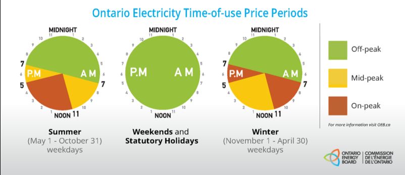
ation approach and the VNS/TS hybrid heuristic.19 Figure 2 Tabu Search Operators 6.1. Test Instances The test instances that are used in the evaluation are based on the ones developed by Schneider et al. (2014) which were constructed using the instances proposed by Solomon (1987). The instances are classified into 3 categories based on the geographical distribution of the customer nodes (see first column of Table 4). The instances that start with “R” are random instances where customers are uniformly distributed, and those that start with “C” are clustered instances in which customers are clustered into small groups. The customer distribution of the “RC” instances is a mixture of random and clustered distributions. The EV fleet is homogeneous, each with a cargo capacity Q = 200, a battery capacity B = 270, and a range of 150 km. The travel speed v is set to a constant value of 30 km/h, and the batteries are recharged at a constant speed α = 1.8. The discharging speed is assumed the same as the charging speed. The choice of these values are discussed in more details in the case study. The locations and time windows in the Schneider instances are normalized values which makes it difficult to relate the charging and discharging time to real-world values so as to estimate the potential costs and gains. We adjust the instances in a way similar to Schiffer and Walther (2018).
20

                                   Table 3   Time-of-Use Electricity Prices
              From          To      Charging Cost (¢/kWh) Discharging Reward (¢/kWh)
            12:00 AM 7:00 AM                   6.5                             6.5
             7:00 AM 11:00 AM                  9.4                             8.0
            11:00 AM 5:00 PM                  13.4                            10.0
             5:00 PM 7:00 PM                   9.4                             8.0
             7:00 PM 12:00 AM                  6.5                            6.5

In particular, we set the maximum distance from the depot to customers/stations as 100 km and
convert all other distances to km proportionally for each instances. In addition, since fully charging
an EV requires B = 270 minutes (4.5 hours), we set the planning horizon as 5am − 12am ([0, 1140]
in minutes) so that an EV has enough time to recharge at night. We scale all time windows
proportionally to minutes to fit the planning horizon. We find through computational experiments
that the time windows in the scaled instances are relatively tight which prevent vehicles from
detouring to perform charging and discharging activities. We thus further relax the time windows
to three periods, morning (5am − 12pm), afternoon (12pm − 6pm), and evening (6pm − 12am),
based on their service start time.
     For charging and discharging, the length of each period is set to one hour, i.e. δ = 60 minutes. The
energy prices which are shown in Table 3 are based on the real time-of-use hydro rate in Ontario,
Canada in effect between May 1, 2019 and October 31, 2019. The reward rates are chosen such
that an EV can make profits by discharging at peak hours (11:00 AM - 5:00 PM) and recharging
the battery later. Note that the reward rates are also economically beneficial to the grid because
the discharging reward that the grid pays to the EV owner is lower than the corresponding market
price.

6.2.     Experimental Setup
All the tests are performed on a MacBook Pro running OS X 10.13.6, using a single 2.30 GHZ
CPU, 16 GB of RAM and CPLEX 20.1.0.0 is used as an optimization solver. The time limit is set
to 7200 seconds and the memory limit is set to 10 GB. The algorithms are implemented as single
thread codes in Python.
     For the VNS/TS hybrid heuristic, the penalty parameters βtw , βbatt , βcargo are set to 10 and the
number of tabu iterations per round is set as ηtabu = 30. The number of VNS iterations ηvns and
the early stopping criterion ηearly are varied with respect to the number of customers included. For
the instances with 5, 10, and 15 customers, ηvns is set to 10, 20, and 30 respectively. ηearly is set to
10 for instances with more than 10 customers and 5 otherwise. For the cyclic operator, Nr is set to
2 when the fleet consists of 3 EVs or less and to 3 otherwise. The length of each exchange block is
randomly selected from {1, 2, 3}. The upper and lower bounds of the tabu tenure are vmin = 5 and
vmax = 15. Parameter κ for the annealing mechanism is set to 0.5.
21
6.3. Computational Results
The results for CPLEX, the VNS/TS heuristic, the Lagrangian relaxation and the LP relaxation
are presented in Table 4. The upper and lower bounds achieved by the four algorithms are presented
in the “UB” and “LB” columns, respectively. The “Time” column indicates the computational
time in seconds. The “Gap” columns indicate the gap between the corresponding upper bound and
the lower bound obtained by the Lagrangian relaxation. Column “Best Iter” indicates the VNS
iteration during which the best solution was found.
Table 4 Performance of CPLEX, Lagrangian relaxation, and VNS/TS heuristic on small instances
Instance CPLEX Heuristic Lagrangian LP Relaxation
Name K UB Time Gap UB Time best iter Gap LB Time LB Time
C101-5 2 481.35 2.05 0.00% 481.35 5.58 9 0.00% 481.35 5.13 -2041.15 0.02
C103-5 2 316.83 1.50 0.00% 316.83 9.16 1 0.00% 316.83 3.39 -1522.90 0.03
C206-5 2 553.42 87.35 0.00% 553.42 10.26 1 0.00% 553.42 33.23 -2533.86 0.03
C208-5 2 471.10 22.58 0.00% 471.10 9.40 1 0.00% 471.10 17.62 -2040.28 0.02
R104-5 2 334.86 21.34 0.00% 349.26 7.33 1 4.30% 334.86 8.03 -2041.51 0.02
R105-5 2 405.05 16.06 0.00% 409.37 12.51 4 1.07% 405.05 5.07 -2042.08 0.02
R202-5 1 530.25 1.13 0.00% 530.25 1.85 2 0.00% 530.25 7.56 -1085.40 0.03
R203-5 2 577.86 251.03 0.00% 577.86 15.90 1 0.00% 577.86 101.93 -2519,02 0.03
RC105-5 2 482.45 261.85 0.00% 482.45 11.42 1 0.00% 482.45 103.90 -2520.12 0.03
RC108-5 2 616.17 57.19 0.00% 616.17 10.82 1 0.00% 616.17 34.30 -2507.49 0.03
RC204-5 1 563.02 32.99 0.00% 579.97 32.52 3 3.01% 563.02 129.35 -1409.40 0.03
RC208-5 1 465.64 0.56 0.00% 465.64 1.41 6 0.00% 465.64 7.75 -1085.40 0.03
C101-10 3 1046.11(∗) 4565.51 32.49% 789.58 62.68 10 0.00% 789.58 2194.74 -4802.90 0.09
C104-10 2 867.31(∗) 952.55 - 702.52 54.62 2 - - >7200.00 -2818.80 0.07
C202-10 2 700.99(∗) 3766.34 15.39% 607.49 91.60 9 0.00% 607.49 >7200.00 -3466.80 0.07
C205-10 3 616.36 4071.78 1.88% 616.36 95.15 3 1.88% 604.98 842.72 -3256.20 0.05
R102-10 4 1090.31(∗) 1976.55 96.01% 561.96 89.80 8 1.02% 556.26 >7200.00 -5022.62 0.08
R103-10 2 458.02(∗) 1463.56 - 443.75 55.05 1 - - >7200.00 -2170.80 0.03
R201-10 2 713.81(∗) 1752.25 20.81% 590.83 46.31 1 0.00% 590.83 >7200.00 -2818.80 0.06
R203-10 2 - - - 742.42 91.92 17 - - >7200.00 -3466.80 0.07
RC102-10 4 1211.21(∗) 1558.34 26.58% 999.48 80.09 2 4.45% 956.87 1931.84 -5037.47 0.10
RC108-10 4 1221.72(∗) 1350.84 57.53% 775.57 135.29 12 0.00% 775.57 >7200.00 -5018.51 0.09
RC201-10 2 850.35(∗) 2041.85 12.02% 761.15 81.25 1 0.27% 759.08 1850.80 -2818.80 0.05
RC205-10 3 1243.35(∗) 1448.82 46.07% 851.21 73.49 2 0.00% 851.21 >7200.00 -4020.07 0.07
C103-15 3 * 2102.03 - 770.22 528.67 14 - - >7200.00 -5200.20 0.15
C106-15 3 670.87(−) >7200.00 - 657.32 320.45 10 - - >7200.00 -3256.20 0.08
C202-15 2 - 3303.37 - 1019.80 271.92 3 - - >7200.00 -3466.80 0.10
C208-15 2 * 2875.61 - 757.12 139.56 2 - - >7200.00 -2818.80 0.07
R102-15 5 * 1975.12 - 692.38 407.32 5 - - >7200.00 -12295.33 0.35
R105-15 4 * 1722.53 - 790.48 392.96 4 - - >7200.00 -7638.94 0.17
R202-15 3 - >7200.00 - 1114.25 299.90 3 - - >7200.00 -5981.33 0.07
RC103-15 4 * 2454.94 - 667.52 495.01 14 - - >7200.00 -6505.45 0.17
RC108-15 3 * 1660.90 - 873.22 206.70 1 - - >7200.00 -5200.20 0.12
RC202-15 3 * 2909.87 - 996.73 267.89 2 - - >7200.00 -5200.20 0.21
RC204-15 3 - >7200 - 971.64 270.05 3 - - >7200.00 -4762.80 0.15
Instances that violate the memory and time limits are labeled with ∗ and − respectively
For the small instances with 5 customers, the VNS/TS heuristic outperforms CPLEX in terms
of solution time for the majority of the tested instances. In terms of bound quality, the Lagrangian
relaxation obtains the optimal solution for every instance, while the LP relaxation yields bounds22
Table 5 Performance of VNS/TS heuristic on medium instances
Instance Heuristic Instance Heuristic
Name K UB Time Best iter Name K UB Time Best iter
C103-20 4 1049.71 1147.21 20 C103-30 4 1059.30 3340.14 2
C106-20 3 833.62 495.04 2 C106-30 4 1724.82 3951.79 7
C202-20 4 1202.31 642.04 1 C202-30 4 1477.16 3615.39 5
C208-20 3 848.83 385.78 1 C208-30 4 1238.15 2798.32 3
R102-20 3 1385.19 713.47 2 R102-30 4 1423.15 3036.66 3
R105-20 4 1257.00 789.36 2 R105-30 4 1895.08 2883.65 4
R202-20 3 1096.58 642.69 3 R202-30 4 1860.16 2447.00 4
RC103-20 3 1152.61 790.07 17 RC103-30 4 1674.06 3182.44 17
RC108-20 4 1358.33 944.22 6 RC108-30 4 1579.86 3998.71 17
RC202-20 3 1545.39 1101.57 11 RC202-30 5 1850.08 3608.25 9
RC204-20 3 996.12 745.32 5 RC204-30 4 1391.72 2297.52 1
C103-25 4 857.06 2191.81 15 C103-35 4 1324.19 5447.90 11
C106-25 3 1329.92 1262.92 11 C106-35 4 1152.76 4954.01 12
C202-25 3 1154.42 1155.89 1 C202-35 4 1759.25 2801.60 2
C208-25 3 1082.15 796.42 2 C208-35 4 1520.57 3924.57 11
R102-25 4 1164.46 1495.67 1 R102-35 4 1928.67 3851.51 8
R105-25 4 1811.40 1088.10 4 R105-35 4 1639.93 2854.46 6
R202-25 3 1209.24 1632.27 17 R202-35 4 1412.07 4365.94 14
RC103-25 4 1372.35 2573.81 16 RC103-35 5 1857.54 3135.70 1
RC108-25 4 1341.98 2416.85 10 RC108-35 5 1786.30 3906.11 2
RC202-25 4 1472.85 2173.26 7 RC202-35 4 1920.45 3047.78 3
RC204-25 4 1644.16 1896.30 3 RC204-35 5 1268.05 6068.46 17
of poor quality. The VNS/TS heuristic obtains the optimal solution for 9 out of 12 instances with
the largest gap being 4.30%.
As the number of customers increases to 10, the performance of CPLEX worsens significantly
where only 1 out of the 12 instances are solved to optimality within the time and memory limits.
CPLEX is able to find feasible solutions for 11 out of 12 instances before termination yet the
gaps are on average 34.31%, which is significantly higher than the average gap of the VNS/TS
heuristic 0.85%. The Lagrangian relaxation obtains bounds for 9 out of the 12 instances and the
gap compared to the upper bound that is found by the heuristic is no more than 4.45%. We note
that solving the Lagrangian subproblem is computationally challenging for the instances with 10
customers and no solution is obtained within the time limits for 3 out of the 12 tested instances.
The lower bounds obtained by the LP relaxation are far away from the optimal values, which
partially explains the low efficiency of CPLEX on this problem.
For the instances with 15 customers, both CPLEX and the Lagrangian relaxation fail to solve
the majority of the instances. CPLEX finds a feasible solution for only 1 out of the 11 instances.
VNS/TS identifies solutions for all the instances within 317 seconds on average.
The results for the VNS/TS heuristic on medium instances are shown in Table 5. The VNS/TS
heuristic is able to solve all the instances with less than 35 customers within 2 hours (20 iterations),
allowing EV operators to implement the proposed approach for real-world tasks that do not require
dynamic EV dispatching. Nevertheless, the proposed VNS/TS heuristic contains a large number ofYou can also read