Time- and energy-resolved effects in the boron-10 based Multi-Grid and helium-3 based thermal neutron detectors - arXiv.org
←
→
Page content transcription
If your browser does not render page correctly, please read the page content below
Time- and energy-resolved effects in the boron-10
                                                   based Multi-Grid and helium-3 based thermal
                                                   neutron detectors
arXiv:2006.01484v2 [physics.ins-det] 14 Jan 2021

                                                                  A. Backisa,b,∗ , A. Khaplanovb , R. Al Jebalib,a , R. Ammerb , I.
                                                                  Apostolidisb , J. Birchc , C.-C. Laib,c , P. P. Deenb,d , M.
                                                                  Etxegaraib , N. de Ruetteb , J. Freita Ramosb , D. F. Förstere , E.
                                                                  Haettnerb , R. Hall-Wiltonb,f,a , D. Hamiltona , C. Höglundb,g , P.
                                                                  M. Kadletzb , K. Kanakib , E. Karnickisb , O. Kirsteinb , S. Kolyab ,
                                                                  Z. Kraujalyteb , A. Lalonib , K. Livingstona , O. Löhmanh , V.
                                                                  Maulerovab,i , N. Mauritzonb,i , F. Müllere , I. Lopez Higuerab , T.
                                                                  Richterb , L. Robinsonb , R. Rothj , M. Shettyb , J. Taylorb , R.
                                                                  Woracekb and W. Xiongb
                                                                  a
                                                                    University of Glasgow, Glasgow, United Kingdom
                                                                  b
                                                                    European Spallation Source ERIC (ESS), Lund, Sweden
                                                                  c
                                                                    Linköping University, Linköping, Sweden
                                                                  d
                                                                    Niels Bohr Institute, University of Copenhagen, Copenhagen, Denmark
                                                                  e
                                                                    Zentralinstitut für Engineering, Elektronik und Analytik, Forschungszentrum Jülich
                                                                  GmbH, Jülich, Germany
                                                                  f
                                                                    Università degli Studi di Milano-Bicocca, Piazza della Scienza 3, 20126 Milano, Italy
                                                                  g
                                                                    Impact Coatings AB, Westmansgatan 29G, SE-582 16 Linköping, Sweden
                                                                  h
                                                                    Technische Universität Darmstadt, Hochschulstraße 8, D-64289 Darmstadt
                                                                  i
                                                                    Lund University, Lund, Sweden
                                                                  j
                                                                    EWCON, Örkelljunga, Sweden
                                                                  E-mail: a.backis.1@research.gla.ac.uk

                                                                  October 2020

                                                     ∗
                                                         Corresponding author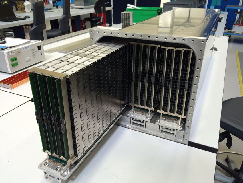
Time- and energy-resolved effects in the boron-10 based Multi-Grid ...                               2

              Abstract. The boron-10 based Multi-Grid detector is being developed as an
              alternative to helium-3 based neutron detectors. At the European Spallation Source,
              the detector will be used for time-of-flight neutron spectroscopy at cold to thermal
              neutron energies. The objective of this work is to investigate fine time- and energy-
              resolved effects of the Multi-Grid detector, down to a few µeV, while comparing it to the
              performance of a typical helium-3 tube. Furthermore, it is to characterize differences
              between the detector technologies in terms of internal scattering, as well as the time
              reconstruction of ∼ µs short neutron pulses. The data were taken at the Helmholtz
              Zentrum Berlin, where the Multi-Grid detector and a helium-3 tube were installed at
              the ESS test beamline, V20. Using a Fermi-chopper, the neutron beam of the reactor
              was chopped into a few tens of µs wide pulses before reaching the detector, located
              a few tens of cm downstream. The data of the measurements show an agreement
              between the derived and calculated neutron detection efficiency curve. The data also
              provide fine details on the effect of internal scattering, and how it can be reduced.
              For the first time, the chopper resolution was comparable to the timing resolution of
              the Multi-Grid detector. This allowed a detailed study of time- and energy resolved
              effects, as well as a comparison with a typical helium-3 tube.

Keywords: Neutron detectors, Gaseous detectors, Boron-10, Multi-Grid detector,
Helium-3, Time resolution
Time- and energy-resolved effects in the boron-10 based Multi-Grid ...                      3

1. Introduction

The European Spallation Source (ESS), is currently under construction in Lund, Sweden
[1, 2, 3]. Due to the sparsity and increased cost of helium-3 gas during the past
two decades [4], as well as the performance limitation due to the expected high flux
from the source, alternatives to the traditional helium-3 based neutron detectors are
being developed. One such alternative is the boron-10 based Multi-Grid detector
[5, 6, 7, 8, 9, 10, 11], invented at the Institut Laue–Langevin (ILL) [12], and jointly
developed with ESS thereafter. The Multi-Grid detector is a large area cold to
epithermal neutron detector, designed for time-of-flight neutron spectroscopy [13] at the
upcoming CSPEC [14] (cold neutron spectroscopy) and T-REX [15] (thermal neutron
spectroscopy) instruments at ESS.
     Neutron spectroscopy is a demanding technique in terms of neutron detector
performance, requiring a high detection efficiency and low noise levels. It also needs
a broad detector coverage, tens of square meters, and hence a low cost per unit active
detector area is important. The spectroscopy information is primarily extracted from
inelastic neutron scattering of a sample, measuring small changes in energy between
incident and scattered neutrons. This probes sample properties such as molecular
vibrations, quantum excitations and motions of atoms. As the measured energy changes
are in the order of meV, the method requires a high time resolution and good knowledge
of interaction location to correctly derive the energy of the scattered neutrons [16, 17, 18].
     For neutron detection, the Multi-Grid detector employs multiple 10 B4 C thin films
coated on aluminum substrates [19, 20, 21]. The 10 B4 C deposition is carried out by the
ESS Detector Coatings Workshop in Linköping, where the deposition is done with an
industrial deposition system, using physical vapor deposition DC magnetron sputtering
[21]. The coated substrates are stacked perpendicularly to the incident neutrons, and
placed in a 3D-position sensitive multi-wire proportional chamber (MWPC), see Section
2.4 for details. Incident neutrons are absorbed in the coating, whereupon one of the
conversion products is ejected into the gas volume. In the gas, charge is released and
collected, and each neutron event is assigned a time-of-flight (tof ), as well as a hit
position. This information is then used to calculate the neutron flight distance (d).
     The neutron time-of-flight and flight distance are relative to a neutron chopper. A
neutron chopper is a device containing an efficient neutron absorber, such as gadolinium
or boron, and is placed blocking the incident neutron beam. The chopper rotates at
a high frequency, and contains an opening for neutrons to pass periodically. That is,
the incident neutron beam is “chopped” into pulses. Each time a neutron pulse is
transmitted, a start time, commonly know as T0 , is recorded. Then, when a neutron is
detected in the detector, a stop time T is acquired. The time-of-flight is then calculated
according to tof = T − T0 , and the neutron flight distance d is the distance between the
chopper and the detection location in the detector, i.e. the hit position.
     Using the time-of-flight and flight distance, the incident neutron energy En can be
calculated on an event-by-event basis. This is done by calculating the neutron velocity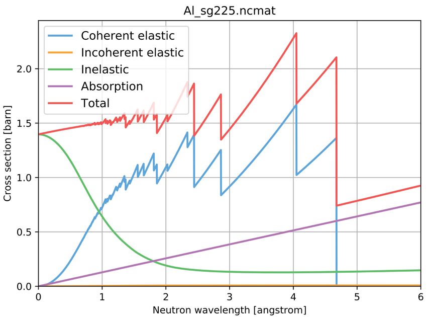
Time- and energy-resolved effects in the boron-10 based Multi-Grid ...                   4

vn , according to vn = d/tof , which gives the energy using En ∝ vn2 . However, a small
fraction of neutrons undergo internal scattering before being detected. This is primarily
due to the aluminum inside the detector, see Section 3.3. Consequently, these scattered
neutrons are assigned an incorrect flight distance, as the additional scattered travel path
cannot be accounted for. This changes the energy line shape reconstruction, adding a
small distribution of neutrons with incorrectly assigned energies [22, 23, 24]. A good
understanding of this effect is important, as spectroscopy instruments depend on a well
understood energy line shape. This is especially true for quasi-elastic scattering analysis
[25], where subtle details in the line shape are studied at the edges of the energy peak.
      For cold neutrons, the detector time and energy resolution are also critical. The
full resolution of the instrument depends on the pulse broadening from the chopper
system, sample scattering and the detector. Therefore, it is desired to keep the detector
energy resolution finer than the resultant resolution of the remaining components. This
is especially important for the slowest neutrons, as the resolution of the chopper system
is highest at these energies. One of the main components of the detector resolution
relates to the uncertainty of when and where the neutron conversion reaction occurs
in the detector. In a helium-3 tube, this reaction can happen anywhere within the
gas, while for the Multi-Grid detector, the reaction can only occur at discrete intervals,
corresponding to the position of the conversion layers [23].
      This work contains three separate investigations, each characterizing an important
aspect of the Multi-Grid detector. First, the neutron detection efficiency of the
Multi-Grid detector is derived and compared to the theoretical prediction. Then, the
magnitude of the internal scattering, as well as the effect it has on the line shape
reconstruction, is investigated. This is done by comparing two different Multi-Grid
prototypes, one with internal topological shielding and one without, and examining the
difference in energy line shape. Finally, the energy resolution of the Multi-Grid detector
and a helium-3 tube are accessed and compared.

2. Instrumentation and experimental setup

The measurements were conducted at the Helmholtz-Zentrum Berlin (HZB), at the BER
II research reactor [26]. At the facility, a series of measurements were done at the V20
beamline [27, 28, 29]. During the course of the measurements, three different detectors
were used: one 10 bar helium-3 tube and two variations of the latest prototype of the
Multi-Grid detector. The setup consisted of a beam-monitor, slits and a lightweight fast
rotating Fermi-chopper [30]. The detectors were situated just after the Fermi-chopper,
as illustrated in figure 2.
      Three direct beam measurements were conducted, one for each of the three
detectors, keeping the rest of the setup constant. In addition to this, two background
measurements were done, one for each of the Multi-Grid prototypes, where the direct
beam was blocked by the helium-3 tube. The helium-3 tube was covered with 5 mm
Mirrobor shielding [31], 80 % B4 C (natural boron) content in weight, at the back.
Time- and energy-resolved effects in the boron-10 based Multi-Grid ... 5
The back-shielding, in combination with the high neutron absorption efficiency of the
helium-3 tube in the measured wavelength range, resulted in transmission levels below
the instrument background level for almost all data points. The exception was for the
data point at 1.2 Å, where the transmission was at the acceptable level of < 5 · 10−4 .
2.1. The ESS test beamline V20
The V20 is a cold to thermal neutron beamline. It was commissioned as an ESS test
beamline, with a chopper system designed to mimic the long pulses which will be
obtained at ESS. This is done by a pair of double disc choppers: a source chopper
and a wavelength band (WB) chopper. Together, these deliver pulses at 14 Hz, 60 ms
pulse width, where the wavelengths in each pulse range from approximately 1 to 10 Å.
The beam line is also equipped with wavelength frame multiplication (WFM) choppers,
which, together with a pair of frame overlap (FOL) choppers, cut the long pulse from the
source chopper to smaller bunches. This option was, however, not used for the herein
reported work, and the corresponding choppers were parked in open position. Instead,
the choppers were used in the “Basic Single Pulse Mode”, as illustrated in figure 1.
ESS Source WFM FOL WB modular neutron FOL Polarizer Optical Benches
Choppers Chopper guide (m=3) Chopper (optional)
Chopper Chopper (Measurement Position)
H=12.5cm, W=6cm
Cold
Source
Basic
Single
Pulse
Mode
Figure 1: Illustration presenting the layout of the V20 beamline, showing the main components and
their locations. At 21.7 m from the moderator, the ESS source chopper is located, which, together with
the WB chopper, cuts the flux into wide pulses at 14 Hz. There are also WFM and FOL choppers,
above presented in blue, followed by an optional polarizer. This allows for two different modes, “Basic
Single Pulse Mode” and “WFM Mode”. For these measurements, single pulse mode was used, which
is illustrated above. The optical benches is where the experiment specific setup is positioned.1
The current setup was assembled at the “Optical Benches” position, at the last
part of the beamline. This is outlined in figure 2, where all the components and their
locations are presented. First, a slit confines the area of the incident neutron beam to a
few cm2 . The incident flux is then recorded by a low helium-3 pressure beam monitor
[32]. After a further slit collimation, halving the beam width, a Fermi-chopper is used
1
Reprinted from “Nuclear Instruments and Methods in Physics Research Section A: Accelerators,
Spectrometers, Detectors and Associated Equipment”, Vol. 839, R. Woracek, T. Hofmann, M. Bulat,
M. Sales, K. Habicht, K. Andersen and M. Strobl, “The test beamline of the European Spallation
Source – Instrumentation development and wavelength frame multiplication”, pp 102-116, 2016, with
permission from Elsevier.Time- and energy-resolved effects in the boron-10 based Multi-Grid ... 6
to cut and shape the long incident pulse to a few tens of µs short pulses. Finally, the
beam is collimated to a 14 × 60 mm2 rectangular beam before reaching the detectors.
This is either the helium-3 tube or the Multi-Grid detector. During the direct beam
measurements with the Multi-Grid detector, the helium-3 tube was removed from the
beam path. Then, during the background measurements, it was re-installed such that
it was blocking the direct beam from reaching the Multi-Grid detector. Note that
the detectors are placed in sequence, due to the limitation of the setup, and that the
Multi-Grid detector is situated approximately an additional 50 % further downstream
of the Fermi-chopper than the helium-3 tube. The signal-to-background ratio at the
instrument is approximately 103 , and is influenced by gamma radiation levels and
straying neutrons in the vicinity of V20.
Multi-Grid detector
Concrete Beam monitor Fermi chopper Helium-3 tube
shielding
Slit 1 Slit 2 Slit 3
80 mm 83 mm 60 mm
30 mm 14 mm
15 mm
Distance from
25.3 m 25.38 m 25.48 m 27.72 m 27.91 m 28.18 m 28.24 m 28.37 m source chopper
Figure 2: Schematic illustration depicting the experimental setup assembled at the optical benches
section at the V20 beamline. The location of the components are shown in relation to the source
chopper. The values mark the center position of the components, except for the Multi-Grid detector,
where it marks the front. The setup includes, downstream from the source, a beam monitor (orange),
a Fermi chopper (green) and slits (black) in between defining a 14 × 60 mm2 rectangular beam. At
the end, either the helium-3 tube (red) or Multi-Grid detector (blue) is used.
2.2. Low pressure helium-3 filled beam monitor
The beam monitor used was a low pressure helium-3 proportional counter [29, 33, 34]
from Eurisys Mesures, currently Mirion Technologies [35]. The detector has an active
area of 100 × 42 mm2 , with a 40 mm active depth. The thickness of the aluminum
window is 4 mm in the neutron beam path, including 2 mm inlet + 2 mm outlet. An
overview of the geometry is seen in figure 3.
The gas-filling is a 1.3 bar Ar-CH4 (90:10 volume ratio) mixture, with a low pressure
of helium-3. The neutron detection efficiency is ∼10−5 at 1.8 Å. Thus, the incident
neutron flux is only marginally reduced, corresponding to the low neutron absorption
in the helium-3 gas and scattering in the 4 mm aluminum window.Time- and energy-resolved effects in the boron-10 based Multi-Grid ... 7
224 mm
61 mm 42 mm ⌀ = 41 mm
100 mm
Figure 3: Low pressure helium-3 filled beam monitor. A drawing of the beam monitor, not to scale,
is presented showing the details of the geometry. The left region (orange and light grey) is a box, while
the middle region (dark grey) is a cylinder, and the right region (black) is a connector.
2.3. Lightweight fast rotating Fermi-chopper
For the measurements, an experimental 120 mm high, 27 mm in diameter, lightweight
Fermi-chopper was used. The purpose was to produce a series of very short, ∼ 10 µs,
and sharp pulses in time, to study the energy dependent scattering within the detector
between pulses. The Fermi-chopper is synchronized to the 14 Hz source chopper
frequency with a clock multiplier of 35, resulting in a 490 Hz rotation frequency. The
chopper uses two rectangular chambers for neutron transmission, and a gadolinium
neutron absorber on the walls. The resulting transmission of the Fermi-chopper is
presented in figure 4. In figure 4a, the time-of-flight spectrum before the Fermi-chopper
is shown, collected using the beam-monitor, while in figure 4b the time-of-flight spectrum
after the Fermi-chopper is shown, collected using the helium-3 tube.
The chopper system produces a series of sharp pulses. However, as can be seen
in figure 4c, there are additional features introduced. First, odd and even peaks are
alternating in intensity. This is due to an asymmetry in the two rectangular Fermi-
chambers, appearing every half rotation of the chopper blades. This is further discussed
in [30]. Second, two distinct side peaks are identified, suppressed by 1-2 orders of
magnitude. The same side peaks are present in data from the Multi-Grid detector.
Thus, this feature is not a detector dependent effect. Additionally, there are 2-3 orders
of magnitude suppressed peaks appearing midway between the main peaks, coinciding
with every quarter rotation of the chopper blades. This was shown to correspond to a
small misalignment of the incident neutron beam, allowing neutrons to pass the side of
the Fermi package every quarter rotation. These peaks does not cause a problem for
the current analysis, as they are easily distinguishable from the main peaks.Time- and energy-resolved effects in the boron-10 based Multi-Grid ... 8
70000
60000 150000
50000
40000 100000
Counts
Counts
30000
20000 50000
10000
0 0
0 20000 40000 60000 0 20000 40000 60000
tof (µs) tof ( s)
(a) (b)
Fraction of chopper rotation: 0 0.25 0.40 0.45 0.50 0.75 0.90 0.95 1
(c)
Figure 4: Time-of-flight spectra before and after the Fermi-chopper. The time offset is arbitrary. In
(a), a spectrum collected with the beam monitor is presented, showing the wide pulse from the source
chopper. In (b), a spectrum from the helium-3 tube is shown, illustrating how the chopper splits the
∼ 60 ms long source pulse into a series of ∼ 10 µs short pulses. In (c), a magnification of a portion of
(b) is shown. On the log scale, it is clear that there are side peaks which are 1-2 orders of magnitude
smaller than the main peaks.
2.4. Helium-3 filled proportional counter
For the measurements, a helium-3 filled proportional counter from Reuter-Stokes [36]
was used. The tube has a total gas pressure of 10 bars, split between 9.85 bar helium-3
and 0.15 bar quenching gas. The active diameter of the tube is 25.4 mm, with a length
of 305 mm, and it is enclosed in 0.51 mm walls of stainless steel. The full geometry
is presented in figure 5. During the measurements, the tube was wrapped in Mirrobor
shielding [31], leaving a small window for incident neutrons.Time- and energy-resolved effects in the boron-10 based Multi-Grid ... 9
Diameter = 25.4±0.8 mm SHV connector
Length = 304.8 ± 1.5 mm
Figure 5: Helium-3 filled proportional counter. A drawing of the tube, not to scale, is presented
showing the details of the geometry.
The tube is a non-position sensitive detector, operated at 1350 V. Gamma events
were rejected using a constant charge discriminator threshold on all events. The read-
out system consists of a multi-channel analyzer, the FAST ComTeC MCA4 [37], which
returns time-of-flight and collected charge for each neutron event. In case of a pile-up
detection during the charge integration process, the event is also assigned a “pile-up
flag”. The shaping time was set to 1 µs.
Note that it was not a strict requirement for the helium-3 tube used in this
measurement to have the specific characteristics described above. The main purpose
of the helium-3 tube was to have a well-understood technology to “bench-mark” the
Multi-Grid detector, while the secondary purpose was to use it as a flux normalization.
The performance comparison with the Multi-Grid detector will, of course, vary if a
different tube is selected. The selected tube, however, is a good choice because it has a
gas pressure representative of what is commonly used for helium-3 tubes in spectroscopy
instruments.
2.5. The Multi-Grid detector
The Multi-Grid detector has a modular design, see for example [5] for a rigorous
description of the detector technology. It consists of a series of identical building blocks
called grids, as shown in figure 6a. In the prototype used here, each grid contains 21
layers of 10 B4 C-coated aluminum substrates, 0.5 mm thick, which are called blades.
The chemical composition and the 10 B-abundance in the 10 B4 C-coatings were analyzed
with Time-of-Flight Elastic Recoil Detection Analysis (ToF-ERDA), performed at the
Tandem Laboratory [38], Uppsala University. The analysis shows ∼79 at.% (atomic
percent) of 10 B and ∼2 at.% of impurity elements (mainly O) in the films, which is
consistent with the values reported in previous publications [19, 20].
The blades are placed in a sequence and oriented orthogonal to the incident
neutrons. The first blade is single-side coated and the remaining twenty double-side
coated. These are the normal blades (blue in figure 6a). Connecting the normal blades
are five support blades, called the radial blades (red in figure 6a). The naming convention
refers to how the blades are oriented related to the incident neutrons. Together, theseTime- and energy-resolved effects in the boron-10 based Multi-Grid ... 10
blades form a grid of cells. The normal blades have three different coating thicknesses,
1 µm, 1.25 µm and 2 µm, where the blades with the thinner coating are at the front
and the ones with thicker coating at the back. If the radial blades are coated, they are
double-side coated with a 1.25 µm coating thickness. At the back of the grid, a 5 mm
thick Mirrobor sheet is placed. The purpose is to absorb the remainder of the incident
neutrons, thus reducing back scattering.
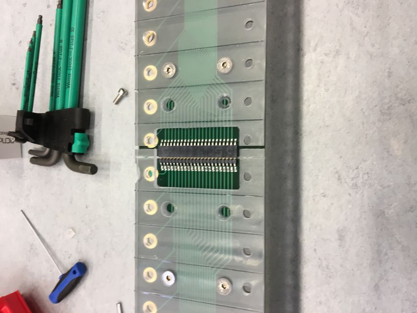
The grids are stacked in three separate columns, see (1) in figure 6b for an example
of a column, where each column contains 40 grids. Between the cells in the grids, anode
wires are stretched, one wire per stack of cells, see (2) and (3) in figure 6b. These
wires are then connected to a high voltage, while the cathode grids are put to ground
potential. By placing the wires and grids in an Ar-CO2 (80:20 volume ratio) filled vessel,
a MWPC is established. The grids, as well as the wires, are electrically insulated from
each other. This results in a position resolution defined by the cell size, where each cell
is 22.5 × 22.5 × 10 mm3 . This is defined as a voxel, and there are a total of 9600 voxels
in the current prototype (40 height × 4·3 width × 20 depth). The corresponding active
detector surface area is approximately 0.24 m2 .
The induced charge released from the boron-10 neutron capture reaction is collected
by the wires and grids. Each neutron event is then assigned a 3D-position based on
coincidences in time between signals from wires and grids. Each event is also assigned a
time-stamp, corresponding to the time-of-flight from the source chopper to the location
of that event within the Multi-Grid detector. Note that each wire is adjacent to at least
two 10 B4 C-coated aluminum substrates, four if the radial blades are coated, and that
incident neutrons can be converted in either one. The information of which coating the
conversion took place is not recorded.
For the measurements, two separate prototypes of the Multi-Grid detector were
used. These prototypes were originally designed and constructed as demonstrators
for measurements at the thermal spectrometer SEQUOIA [17] in August 2018, at
the Spallation Neutron Source (SNS) [39]. The prototypes are therefore optimized
for thermal neutron energies. The two prototypes are identical in all aspects, except
for the grid specifications, which are summarized in table 1. The grids in Detector
1 is made with radiopure aluminum from Praxair [40], with less than 1 ppb (parts
per billion) radioactive impurities such as Th and U, while the grids in Detector 2 is
made with commercially available Al5754. The impact of radioactive impurities in the
Al5754 alloy, such as Th and U, is alpha emissions which raises the time-independent
background level in the detector [10]. Furthermore, the impact of parasitic reactions
due to neutron absorption in the remaining elements in the alloy, most prominently
manganese, is a photon yield (cm−3 s−1 ) 1 order of magnitude below that of aluminum
[24]. These effects, however, do not impact the current measurements, as the extra flat
background can be subtracted and the photon events removed using a software cut.
For these measurements, the parameter of interest is the 10 B4 C-coating on the radial
blades, see figure 6a. This coating is only present in Detector 2.
The purpose of coating the radial blades is to reduce the effect of internally scatteredTime- and energy-resolved effects in the boron-10 based Multi-Grid ... 11
2 μm 1.25 μm
1
1.25 μm
…
1 μm
…
3
Normal blade 2
Radial blade
(a) (b)
Figure 6: Pictures depicting the internal structure of the Multi-Grid detector. In (a), the basic
building block of the detector, a grid, is shown. An example of a normal (blue) and a radial (red) blade
is presented in the figure. The coating thicknesses of the different blades are shown within the blue
and red brackets. The 5 mm Mirrobor sheet is seen at the back. In (b), it is shown how the grids are
stacked in three rows and inserted into the vacuum tight gas vessel. Point (1) shows the 40 stacked
grids, point (2) shows the 4 wire rows, and point (3) shows the 20 wire layers. Incident neutrons are
presented as blue arrows in both pictures.
Table 1: Summary of grid specifications relevant for internal scattering for the two Multi-Grid
detectors used during the measurements.
Detector 1 Detector 2
Radiopure aluminum Yes No
10
B4 C-coated radial blades, 1.25 µm No Yes
neutrons. By adding the extra coating, scattered neutrons can be absorbed more
quickly. This reduces the average extra flight distance by scattered neutrons, which
in turn improves the accuracy of the energy reconstruction. In addition to this, the
overall neutron detection efficiency for incident divergent neutrons, i.e. incident neutrons
traveling at a path crossing the radial blades, is increased. This is due to the additional
converter material introduced. As a consequence, neutrons are statistically absorbed
closer to the detector entrance, reducing the travel path through aluminum within the
detector. This lowers the number of interaction opportunities in aluminum, reducing
the overall amount of internally scattered neutrons. This further improves the accuracy
of the energy reconstruction.
The read-out electronics is the mesytec VMMR-8/16 [41], which can handle 2048
channels simultaneously. In this setup, 360 channels are used, corresponding to the
80 · 3 = 240 wires and 40 · 3 = 120 grids. The data is transported using optical fibres.
Each recorded event contains channel id, related to the wire or grid which collected
the charge, as well as the time-of-flight (46 bits) and collected charge (12 bits). All
events which occur within a pre-defined coincidence window are received together. ATime- and energy-resolved effects in the boron-10 based Multi-Grid ... 12
majority of the events consist of one wire and a few grids. By combining coincidences
between wires and grids, neutron events are reconstructed with a (x, y, z)-hit location,
time-of-flight and collected charge. If more than one grid fired within coincidence, the
grid with the most collected charge is used for the position reconstruction.
3. Method and analysis
This study concerns three properties of the Multi-Grid detector: neutron detection
efficiency, internal neutron scattering, and time- and energy resolution. For the efficiency
and resolution analysis, data from Multi-Grid Detector 1 are used, while for the
scattering analysis data from both Detector 1 and 2 are needed. The method and
analysis procedure is described below, starting with a reduction of the raw data by an
event selection procedure.
3.1. Event selection
The Multi-Grid detector is designed for cold- to epithermal neutron detection. However,
as the detector also has a certain low, but not negligible, gamma sensitivity [42], it is
necessary to remove gamma events before proceeding with the analysis. This is done
by studying the pulse height spectra (PHS), which shows the distribution of charge
collected from events in the detector.
Gamma events have a clear signature in PHS. This is presented in figure 7a, where
the PHS (x-axis) is plotted for each grid (y-axis). The y-axis is expressed in electronic
channels, where Grid 80 is at the bottom and Grid 119 at the top (channel 0 to 79 are
reserved for wires). The x-axis is expressed in 12 bit analog-to-digital converter (ADC)
channels, ranging from 0 to 4095. The gamma events are concentrated in a distribution
at the low ADC values, 100 to 500 ADC channels, while neutrons span the full range.
Notably, neutrons from the direct beam are seen hitting only three grids at the lower
part of the detector, as shown by the three horizontal red stripes.
There is an elevated noise level in the middle grid, Grid 99, where the events cover
a larger range in the PHS. This middle grid sits directly on top of a junction between
the two unshielded PCB connectors connected halfway up the detector, see figure 7b.
The increased rate could, therefore, be due to crosstalk between the exposed connectors
and the grid. Alternatively, a local physical offset would put the wire closer to the
center grid, which would increase the gain there in a discrete step. As the nominal
pitch between grids and wires is only 5 mm, a deviation on the fraction of mm would
be sufficient to cause a noticeable effect.
For the purpose of the following analysis, the exact distribution of the gamma
spectrum is not critical. Here, a constant ADC software threshold at 600 ADC channels
is applied, such that the gamma events are rejected. However, for the scattering analysis,
a more aggressive ADC cut is required to clean the data further. This is because the
rate of scattered events is, in the middle region of the detector at parts of the lambdaTime- and energy-resolved effects in the boron-10 based Multi-Grid ... 13
Gamma events Grid channel:
96 97 98 99 100 101 102 103
Direct neutrons
(b)
(a)
Figure 7: Event selection on data from the Multi-Grid detector. In (a), the PHS (x-axis) are shown
for all individual grids (y-axis). The numbering refers to the electronic channels related to the grids,
where Grid 80 is at the bottom and Grid 119 at the top. In the figure, data from Detector 1 is used
as an example. In (b), the exposed PCB connectors are shown. The center grid, Grid 99, is placed
directly above the connectors.
spectrum, comparable to the elevated noise rate. Fortunately, the noise events are
concentrated at the low ADC values, while the scattered neutron events span the full
ADC range. Therefore, a cut at 1200 ADC channel is used instead for the scattering
analysis, which removes the remainder of the noise present in the middle grid, while
keeping a majority of the events from scattered neutrons.
In addition to the ADC-cuts, a multiplicity cut is performed. The multiplicity
of an event denotes the number of wires and grids which fired within the coincidence
window. As the conversion products have a finite range, there is a limit on how large
multiplicities proper neutron events can have. Therefore, a study of the multiplicity can
be used as an additional filter to remove gamma events and false coincidences. For this
study, events with wire multiplicity 1 and grid multiplicity 1 to 5 is kept. The maximum
grid multiplicity is larger than that for wires, as the released charge spread more easily
to adjacent grids than adjacent wires.
3.2. Efficiency
Neutron detection efficiency is defined as the fraction of incident neutrons which are
detected, i.e. the number of detected neutrons divided by the total number of incident
neutrons. This is described in equation (1),
S detected
= , (1)
S incident
where is the neutron detection efficiency, S detected is the sum of detected neutrons
and S incident is the sum of incident neutrons. For the Multi-Grid detector, the quantity
detected incident
SM G is accessed from the number of counts in the data, while SM G is not measuredTime- and energy-resolved effects in the boron-10 based Multi-Grid ... 14
directly. Instead, it is estimated from a separate measurement with the helium-3 tube.
Using these two measurements, one with the Multi-Grid detector and one with the
helium-3 tube, the neutron detection efficiency for the Multi-Grid detector is derived.
incident
The incident neutrons on the Multi-Grid detector SM G , i.e. integrated absolute
flux, is calculated according to equation (2),
incident detected 1 BMM G
SM G = SHe−3 · · , (2)
He−3 BMHe−3
detected
where SHe−3 is the detected neutrons in the helium-3 tube and He−3 is the calculated
efficiency of the helium-3 tube. BMM G is the integrated beam monitors counts over
the full wavelength spectrum from the measurement with the Multi-Grid detector, and
BMHe−3 the corresponding number from the separate run with the helium-3 tube. The
detected
inverse of the helium-3 efficiency is used to scale SHe−3 to approximate the total
incident
number of neutrons incident on the detector, SHe−3 . The fraction of the beam monitor
counts is then used to scale this value to make it comparable to the integrated flux on
the Multi-Grid detector. That is, it accounts for the difference in flux during the two
separate measurements.
Inserting equation (2) into (1), a formula for deriving the Multi-Grid efficiency as
a function of the incident neutron wavelength λn is thus written according to equation
(3),
−1
detected detected 1 BMM G
M G (λn ) = SM G (λn ) · SHe−3 (λn ) · · , (3)
He−3 (λn ) BMHe−3
where M G (λn ) is the derived Multi-Grid efficiency.
detected detected
SM G (λn ) and SHe−3 (λn ) are calculated by integrating counts above background
for each peak from the Fermi-chopper in the wavelength spectra. This is presented in
figure 8.
As the experimental setup does not produce well defined peaks, recall the parasitic
peaks shown in figure 4c, there is an uncertainty on the correct way to integrate the
peak area. This uncertainty is accounted for by introducing two intervals: one very
narrow, ±σ, encompassing only the peak center, and one wide, encompassing the full
peak, as well as any parasitic peaks. By using the narrow interval, effects from the
parasitic peaks can be rejected. However, this also means that any differences in peak
shape between the Multi-Grid detector and helium-3 tube are not accounted for. By
using the two intervals, an estimate of this systematic uncertainty on the efficiency is
obtained.
The peak areas are presented in figure 8c as a function of wavelength, where the
areas from the narrow- (red) and wide (blue) are presented together. The highest fluence
rate in the spectra, at around 2.5 Å, is approximately 2 · 106 s−1 cm−2 . The fluence
rate in the peak was estimated using data from the beam monitor, located a few meters
upstream from the helium-3 tube.Time- and energy-resolved effects in the boron-10 based Multi-Grid ... 15
Multi-Grid detector, 3.6 Å Helium-3 tube, 3.6 Å
105 Gaussian fit 105 Gaussian fit
Background Background
estimation estimation
Wide interval, Wide interval,
104 [-30 , 60 ] 104 [-30 , 60 ]
Narrow interval, Narrow interval,
[-1 , 1 ] [-1 , 1 ]
Counts
Counts
Multi-Grid detector Helium-3 tube
103 103
102 102
6.1 6.2 6.3 6.4 6.1 6.2 6.3 6.4
Energy (meV) Energy (meV)
(a) (b)
1400000 1.0
Peak area
1200000 Multi-Grid detector, wide peak interval
Helium-3 tube, wide peak interval 0.8
1000000 Multi-Grid detector, narrow peak interval
Peak area (counts)
Helium-3 tube, narrow peak interval
Pile-up fraction
800000 0.6
600000 0.4
400000
0.2
200000 Helium-3 tube
Pile-up fraction
0 0.0
1 2 3 4 5 6 7
Wavelength (Å)
(c)
Figure 8: Peak areas used for efficiency calculation. In (a) and (b), an example of peaks at 3.6 Å are
presented for the Multi-Grid detector and helium-3 tube. In the plots, the Gaussian fit (dotted black),
the background estimation (dashed black) and the narrow- (red) and wide (blue) integration intervals
are also presented. In (c), integrated peak area is shown as a function of neutron wavelength. The peak
area for the Multi-Grid detector (squares and diamonds) and helium-3 tube (triangles) is presented for
the narrow peak interval (red) and wide peak interval (blue). The fraction of pile-up events encountered
in the helium-3 read-out system (green) is plotted on the separate right-hand y-axis.
He−3 (λn ) is calculated to account for the absorption in the gas and the scattering in
the stainless steel tube. If a neutron is absorbed, it is considered detected. The neutron
absorption probability is determined using the helium-3 absorption cross-sections, gas
pressure, and neutron travel distance in the tube. The travel distance depends on where
the neutron hits the tube along the tube diameter, i.e. the neutron has a longer travel
distance if it hits the center of the tube than at the edge, and the calculation accounts
for this by using the average perpendicular tube depth as neutron travel distance. The
acquired absorption probability is then scaled by the fraction of the incident neutron
flux lost due to scattering in the steel tube. This fraction is estimated as the scattering
probability scaled by the heuristic factor 0.5, as not all neutrons which scatter are lost.
Corrections for factors such as wall effect and dead zones in the gas are not taken into
account in this approximation.Time- and energy-resolved effects in the boron-10 based Multi-Grid ... 16
In figure 9a, the calculated efficiency is plotted as a function of position along
the tube diameter, together with measurement data from a previous measurement
[43, 44]. The data agree to within a few percentages, confirming the validity of the
calculation. The offset is accounted for in later calculations as a systematic uncertainty.
In figure 9b, the average efficiency across the tube diameter is shown as a function of
neutron wavelength. Two curves are presented, one with the beam centered on the tube
and one with a 5 mm offset. This is to account for the systematic uncertainty of beam
alignment, which is taken into consideration in later calculations.
1.0 1.0
0.8 0.8
0.6
Efficiency
0.6
Efficiency
0.4 Data 0.4
Beam profile Calculation
0.2 Calculation 0.2 Beam position: ±0 mm
Measurement Beam position: ±5 mm
0.0 0.0
10 5 0 5 10 0 2 4 6
Position (mm) Wavelength (Å)
(a) (b)
Figure 9: Neutron detection efficiency of the helium-3 tube. In (a), the efficiency at 2.5 Å is shown
as a function of displacement from the tube center. The neutron beam width (red lines) is shown
together with the calculation (black line) and data (black points), which was gathered during a previous
measurement at ILL. In (b), the calculated efficiency is presented as a function of wavelength. Each
value is averaged over the tube width hit by the beam, showing it centered (red) and at ±5 mm offset
(blue).
In figure 10, the beam monitor data are plotted, corresponding to the separate
measurements with the Multi-Grid detector and helium-3 tube, BMM G and BMHe−3 ,
respectively. In figure 10a, the rates are shown, while in figure 10b the fractional rate,
BMM G /BMHe−3 , is presented. It is seen that incident flux during the two measurements
were similar, as the fraction is only a few percentages below 1. It is also seen that the
fraction is wavelength independent within a few percentages. The high uncertainty
around 1 Å is due to poor statistics.
The derived Multi-Grid efficiency is presented in figure 11. In the plot, the derived
efficiency for the two integration intervals (red and blue) are compared to the analytical
prediction (black). The error bars show systematic uncertainties. The calculation for the
analytical prediction includes the attenuation of neutrons in aluminum, the absorption
probability in the 10 B4 C-coating, as well as the escape probability of the conversion
products from the coating. The incident neutrons are assumed to hit the front of the
detector at a perpendicular angle. All calculations are based on derivations presented
in [45, 46, 47]. The width of the curve indicates the systematic uncertainty on the
calculation, based on the uncertainty on the input parameters, as well as flux loss dueTime- and energy-resolved effects in the boron-10 based Multi-Grid ... 17
Beam monitor rate 1.10 Fractional beam monitor rate
1.2 BMMG/BMHe 3
1.0 1.05
Count rate (s 1)
3
0.8
BMMG/BMHe
0.6 1.00
0.4
0.2 BM, Multi-Grid run (BMMG) 0.95
BM, Helium-3 run (BMHe 3)
0.0 0.90
1 2 3 4 5 6 7 1 2 3 4 5 6 7
Wavelength (Å) Wavelength (Å)
(a) (b)
Figure 10: Beam monitor data corresponding to the two different measurements, one with the Multi-
Grid detector (blue) and one with the helium-3 tube (red). In (a), the histogrammed beam monitor
counts, normalized by measurement duration, are presented as a function of neutron wavelength. In
(b), the fractional rates, Multi-Grid detector over helium-3 tube, are shown.
to scattering in the aluminum window.
Referring to figure 11, it is seen that for long wavelengths, 4 to 6 Å, the derived-
and calculated efficiency agree well within the uncertainties. For wavelengths shorter
than 4 Å (highlighted grey area), a strong deviation from the calculation is seen. This
is due to the saturation of the helium-3 detector system. The highest fluence rate in the
spectra is high enough, > 106 s−1 , to cause multiple hits within the 1 µs shaping time of
the read-out system. This is seen from the fraction of pile-up events in the tube (green),
which follows the observed deviation. An additional reason is that the data transfer
speed limit per channel, ≈ 106 events s−1 , is similar to the peak flux, which might cause
loss of data. This could have been prevented by using a lower incident flux. However,
as the scattering analysis requires the best possible signal-to-noise ratio, a high neutron
flux was essential.
An attempt was made to account for the saturation in the helium-3 tube using
information of the incident flux and shaping time. This is presented for the wide peak
interval (orange crosses) and the narrow peak interval (green diamonds). The procedure
allows for a few more data points to be within uncertainties. However, the correction
is not strong enough for the majority of data points within the saturated region. This
could be because the incident flux is sufficiently intense to introduce additional effects
in the helium-3 tube, such as space charge effects, which further decreases the efficiency.
As these additional effects are not accounted for in the correction, a deviation is still
seen.
The saturation process is also the cause of the strong staggering effect between 2 and
3 Å. In figure 8c, it is seen how the Multi-Grid detector (squares and diamonds) follow
the intensity from Fermi-chopper, i.e. every other pulse is more intense, even where
the flux is at the highest level. This is not the case for the helium-3 tube (triangles),
which is flat between 2 and 3 Å. As the oscillations between adjacent data points in theTime- and energy-resolved effects in the boron-10 based Multi-Grid ... 18
two detectors no longer match in this region, the fraction of the peak areas is not flat,
as it is above 4 Å. The saturation effect seen in the helium-3 detector is absent in the
Multi-Grid detector.
1.8 1.0
Multi-Grid detector
1.6 Calculated efficiency
1.4 Derived efficiency, wide peak interval 0.8
1.2 Derived efficiency, narrow peak interval
Pile-up fraction
Derived efficiency, wide peak interval (corrected) 0.6
Efficiency
1.0 Derived efficiency, narrow peak interval (corrected)
0.8
0.4
0.6
0.4 Helium-3 tube 0.2
0.2 Pile-up fraction
Unusable region
0.0 0.0
1 2 3 4 5 6 7
Wavelength (Å)
Figure 11: Derived Multi-Grid efficiency (blue circles and red triangles) plotted against the calculated
efficiency (black band). The width of the black band shows the uncertainty range of the efficiency
calculation. In plot, the derived efficiency where the helium-3 data has been corrected to account for
the saturation in the helium-3 tube (orange crosses and green diamonds) are also shown. The fraction
of pile-up events encountered in the helium-3 read-out system (green crosses) is plotted on the separate
right-hand y-axis. The grey region covers the unusable portion of the data, caused by saturation in the
helium-3 detector system.
3.3. Internal neutron scattering
The main source of internal neutron scattering in the Multi-Grid detector is caused by
the presence of aluminum [22]. The other elements in the neutron beam path, boron
and carbon in 10 B4 C, have a negligible effect. This is because 10 B4 C, although having a
2-3 times higher scattering cross-section than aluminum in the measured energy range
[48], have over two orders of magnitude thinner total thickness compared to aluminum
(60 µm and 14.5 mm, respectively, for neutrons incident perpendicular on the detector
surface).
Aluminum has a periodic crystal structure, like any other crystalline solid, which
allows for coherent scattering of atoms within the same crystal lattice, as well as
incoherent scattering from the individual atomic nuclei. The neutron interaction cross-
sections in aluminum are presented in figure 12a, generated using NCrystal [49]. It is
seen that for wavelengths between 1 and approximately 4.7 Å, coherent elastic scattering
is dominant. The cut-off wavelength at 4.7 Å, where the coherent elastic scattering
drops to zero, indicates the maximum wavelength where diffraction occurs in the crystal
structure, i.e. the maximum wavelength where the Bragg condition is fulfilled for the
aluminum crystal lattice. For wavelengths longer than this, no coherent scattering
occurs. An example of internal neutron scattering is presented in figure 12b.Time- and energy-resolved effects in the boron-10 based Multi-Grid ... 19
22 cm
9 cm
Direct neutron
Scattered neutron
(b)
(a)
Figure 12: Neutron scattering of aluminum. In (a), cross-sections for different neutron interactions
with aluminum is presented. These include elastic scattering (blue and orange), inelastic scattering
(green), absorption (purple), as well as the total cross-section (red). The figure is generated using
NCrystal [49]. In (b), an illustration of internal scattering is shown, where an incident neutron (blue) is
scattered (red). The radial blades are highlighted in orange, which can be either coated or non coated
with 10 B4 C.
The impact of the scattered neutrons shows as an added time-dependent
background in the detector. This is caused by an incorrect energy reconstruction of
the scattered neutrons. The neutron energy, En , is determined according to equation
(4),
2
mn d
En = · , (4)
2 tof
where mn is the neutron mass, d is the source-to-detection distance, and tof is the
corresponding time-of-flight. However, as the distance d is based on the detection
voxel, this distance will be incorrect if the neutron is scattered before being detected.
Moreover, as the neutron might acquire an additional flight time between scattering
and detection, or a shortened flight time if the neutron gained energy through inelastic
scattering in aluminum (green cross-sections in figure 12a), this further distorts the
energy reconstruction. Therefore, a scattered neutron has an energy reconstruction
dependent on equation (5),
2
mn d ± δd
En0 = · , (5)
2 tof ± δT
where En0 is the reconstructed energy for an internally scattered neutron, ±δT is the
change in the flight time between scattering and detection, and ±δd is the change
in assumed distance due to the incorrect voxel detection. Due to the large mass
difference between aluminum nuclei and neutrons, most scattering can be consideredTime- and energy-resolved effects in the boron-10 based Multi-Grid ... 20
elastic. Consequently, δT will predominantly be positive, corresponding to the extra
flight time between scattering and detection. Therefore, internally scattered neutrons
will predominately be reconstructed with an energy En0 < En . The exception to this
is when a neutron gains energy through inelastic scattering and is scattered forward
with a sufficiently small deviation, so that δd is small. In this case, the neutron will be
detected earlier than if it would not have been scattered, hence δT < 0 and En0 > En .
To minimize the impact of scattered neutrons on the energy line shape, the
additional flight distance between scattering and detection should be kept as short as
possible. This reduces δd and δT in equation (5), closing in to the ideal case in equation
(4). To facilitate this, 10 B4 C-coating on the radial blades in the grids can be introduced
(figure 12b, orange lines).
To investigate the effect of the radial coating, data from Detector 1 (non-coated
radial blades) and Detector 2 (coated radial blades) are compared. As the neutron
beam is highly collimated, recorded events from scattered neutrons (figure 13a and 13b,
long green stripes) can be separated from those from the direct beam. This is achieved
by performing a geometrical cut, removing all events in the direct beam (grid 87-89,
row 6) and keeping the scattered neutrons (everything outside grid 87-89, row 6). The
volume outside the direct beam region is called the beam periphery. Note that there
are scattered neutrons in the beam region as well, and that these are rejected in this
approach. This is not an issue, however, as an absolute measure of scattering is not
intended, only a comparison between Detector 1 and Detector 2.
To verify that the events seen at the beam periphery are indeed internally scattered
neutrons, and not from a beam halo or a similar effect, the background data is used.
This is presented in figure 13c and 13d, which shows data recorded when the direct
beam was blocked with the helium-3 tube. The helium-3 tube, 25 mm in diameter, is
wide enough to stop the direct beam. However, it does not have a sufficient solid angle
coverage to make a prominent blocking of a potential halo effect. That the long green
lines in figure 13a and 13b is only seen when the helium-3 tube is removed from the
direct beam, demonstrates that the effect must originate after the helium-3 tube. As
the only component after the helium-3 tube is the Multi-Grid detector, this shows that
the lines originate from scattering in the detector.
Studying data with two different cuts, full data versus no direct beam, the
wavelength distribution is acquired for Detector 1 and 2. This is presented in figure 14.
The blue and green histograms are from the full data, while the red histograms are from
data where the direct beam is cut. Overlaying the curves allows for a visualization
of the magnitude of scattered neutrons and how it depends on wavelength. The
black histograms are from the corresponding background measurements, which has an
additional normalization based on the time-independent background level in the facility.
This rate is seen in the flat region between 0 and 0.5 Å, and depends on the overall
activity in the vicinity of V20, which cannot be account for by the beam monitor data
alone. It is noted that the background data has no time correlation with the Fermi-
chopper, i.e. an absence of sharp peaks.Time- and energy-resolved effects in the boron-10 based Multi-Grid ... 21
Beam not blocked Beam not blocked 10 1
10 2
60000
110
Normalized counts
Normalized counts
10 2
10 3
40000
tof (µs)
100
Grid
10 4 10 3
90 20000
10 5
10 4
80 10 6 0
0 20000 40000 60000 0 5 10
tof (µs) Row
(a) (b)
Beam blocked Beam blocked 10 1
10 2
60000
110
Normalized counts
Normalized counts
10 2
10 3
40000
tof (µs)
100
Grid
10 4 10 3
90 20000
10 5
10 4
80 10 6 0
0 20000 40000 60000 0 5 10
tof (µs) Row
(c) (d)
Figure 13: Histograms comparing data from the Multi-Grid detector when the beam was not blocked,
(a) and (b), and blocked, (c) and (d). The two left plots show counts in grids vs. time-of-flight, while
the two right plots show counts in rows vs. time-of-flight. The counts have been normalized to the
accumulated beam monitor counts from the corresponding run. Note that Detector 1 is used in this
example, but the same conclusions are drawn if Detector 2 is studied.
To study the energy line shape in detail, a peak at approximately 1.47 Å from
Detector 1 is used as an example, see figure 15. In figure 15a, histograms over energy
are presented. Again, the blue histogram is from the full volume, the red histogram is
from the beam periphery, and the black histogram is from the background measurement.
Overlaying the curves allows for a clear visualization of how the scattered neutrons
affect the shape of the peak. It is observed that the majority of scattered neutrons are
reconstructed with a lower energy than the peak mean, resulting in a “shoulder” on the
left side of the peak.
From the long green lines in figure 13a, it is seen that the maximum distance the
scattered neutron travel within the detector is approximately 15 grids, corresponding to
about 30 cm. To estimate where these scattered neutrons are reconstructed in the
energy spectra, equation (5) is used. This is done by using the peak mean as an
approximation of the incident neutron energy, while assuming elastic scattering and
that δT is the dominant contribution to the distortion of the energy reconstruction.Time- and energy-resolved effects in the boron-10 based Multi-Grid ... 22
Detector 1 (non-coated radial blades) Detector 2 (coated radial blades)
10 1 Beam not blocked (full volume) 10 1 Beam not blocked (full volume)
Beam not blocked (beam periphery) Beam not blocked (beam periphery)
Beam blocked (beam periphery), Beam blocked (beam periphery),
normalized with time-independent normalized with time-independent
background level background level
Normalized counts
Normalized counts
10 2 10 2
10 3 10 3
10 4 10 4
0 2 4 6 8 10 0 2 4 6 8 10
Wavelength (Å) Wavelength (Å)
(a) (b)
Figure 14: Histograms over wavelength for the two Multi-Grid detectors. In (a), Detector 1 (non-
coated radial blades) is shown, while in (b), Detector 2 (coated radial blades) is presented. Using data
from when the beam was not blocked, two separate histograms are shown in each plot: data from the
full volume (blue and green) and beam periphery (red). The background data (black) is also based on
the beam periphery region. The plots are normalized by accumulated beam monitor counts from the
individual runs. The background data has an additional normalization based on the time-independent
background level during the separate measurements.
The colored vertical lines in figure 15a shows the result of this analysis, which overlaps
well with the location of neutrons detected in the beam periphery (red).
A comparison in the energy line shape with data from the helium-3 tube is presented
in figure 15b. Four histograms are shown, three from the Multi-Grid detector and
one from the helium-3 tube. The separate histograms from the Multi-Grid detector
corresponds to the full data, beam periphery, and beam center. On the left side of the
peak, it is seen that the helium-3 data overlap well with the data from the beam center
of the Multi-Grid detector (compare orange and green). This further validates that the
peak shoulder in the full data (blue) is due to scattered neutrons. Note that there is
additional broadening in the data from the Multi-Grid detector, as it was further away
from the Fermi-chopper than the helium-3 tube. This also affects the parasitic peak on
the right side of the peak center, which is present in both data sets but broader for the
Multi-Grid detector.
To quantitatively compare Detector 1 and 2 in terms of internal scattering, a
figure-of-merit, f om, is introduced. This is defined as the number of counts above
background at a specified interval away from the peak center, divided by the peak area.
The background is estimated to be locally flat, i.e. constant in energy, over the peak
width. It is calculated on a peak-by-peak basis, based on the rate at the side of the
peak. The reason the background measurements is not used for background subtraction
is because of non-negligible systematic offsets. This is seen in figure 14a and 14b, where
the background (black) does not follow the “bump” at 3 Å equally well.
The definition of the chosen f om is presented in equation (6),Time- and energy-resolved effects in the boron-10 based Multi-Grid ... 23
Peak @ 1.47 Å Peak @ 1.47 Å
Flight: +0 cm 100 Multi-Grid detector
Flight: +5 cm (full data)
Flight: +10 cm Multi-Grid detector
10 3 (beam periphery)
Counts normalized to maximum
Flight: +15 cm 10 1
Flight: +20 cm Multi-Grid detector
Flight: +25 cm (beam center)
Normalized counts
Flight: +30 cm Helium-3 tube
10 4 Full data 10 2
Beam periphery
Background
10 3
10 5
10 4
10 6
37 38 39 37 38 39
Energy (meV) Energy (meV)
(a) (b)
Figure 15: Effect on peak shape by internally scattered neutrons at 1.47 Å in the Multi-Grid detector
(Detector 1). Histograms from the full data in the Multi-Grid detector (blue), the beam periphery
(red) and beam center (green) is seen, together with the background data (black) and helium-3 data
(orange). In (a), the approximated location of scattered neutrons are shown as vertical lines. Each line
corresponds to the energy reconstruction for scattered neutrons with a specific extra travel distance
within the detector, as specified in the legend. The counts in the histograms are normalized to the
accumulated beam monitors counts. In (b), the Multi-Grid detector is compared with the helium-3
tube. The helium-3 data has been artificially shifted along the energy-axis, such that it is aligned with
the peak center of the Multi-Grid detector. This is to facilitate peak comparison. The counts are
normalized to peak maximum.
E2
1 X
f om = · (counts − background), (6)
peakarea E
1
where peakarea is the peak area within ±5σ (using data from the full volume), E1 and E2
are the energy interval limits, counts is the number of counts in the beam periphery, and
background is the flat background estimation. That is, the f om captures the background
subtracted counts at the edge of the peak, as a fraction of the peak area. Consequently,
a small f om is desirable, as this implies a low amount of scattered neutrons in the
specified energy range. In words, the f om can be approximately stated as:
shoulder area
f om = .
peak area
The limits E1 and E2 should be selected on a peak-by-peak basis, such that the same
peak region is scanned for all peaks across the wavelength spectra. Unfortunately, this is
not a trivial task, as the peak shape changes with wavelength. This also complicates the
comparison in f om between different instruments, such as studies done at SEQUOIA
and CNCS [11, 39], as the peak shape is heavily dependent on the resolution of the
chopper system. Here, the peak shoulder is split into approximately three equally sizedYou can also read