Quantifying Long-Term Urban Grassland Dynamics: Biotic Homogenization and Extinction Debts - MDPI
←
→
Page content transcription
If your browser does not render page correctly, please read the page content below
sustainability

Article
Quantifying Long-Term Urban Grassland Dynamics:
Biotic Homogenization and Extinction Debts
Marié J. du Toit 1, * , D. Johan Kotze 2 and Sarel S. Cilliers 1
 1    Unit of Environmental Sciences and Management, North-West University, Potchefstroom Campus,
      Private Bag X6001, Potchefstroom 2520, South Africa; Sarel.Cilliers@nwu.ac.za
 2    Faculty of Biological and Environmental Sciences, Ecosystems and Environment Research Programme,
      University of Helsinki, Niemenkatu 73, FI-15140 Lahti, Finland; johan.kotze@helsinki.fi
 *    Correspondence: 13062638@nwu.ac.za; Tel.: +72-18-2992523

 Received: 27 December 2019; Accepted: 15 February 2020; Published: 5 March 2020

 Abstract: Sustainable urban nature conservation calls for a rethinking of conventional approaches.
 Traditionally, conservationists have not incorporated the history of the landscape in management
 strategies. This study shows that extant vegetation patterns are correlated to past landscapes
 indicating potential extinction debts. We calculated urban landscape measures for seven time periods
 (1938–2019) and correlated it to three vegetation sampling events (1995, 2012, 2019) using GLM
 models. We also tested whether urban vegetation was homogenizing. Our results indicated that
 urban vegetation in our study area is not currently homogenizing but that indigenous forb species
 richness is declining significantly. Furthermore, long-term studies are essential as the time lags
 identified for different vegetation sampling periods changed as well as the drivers best predicting
 these changes. Understanding these dynamics are critical to ensuring sustainable conservation of
 urban vegetation for future citizens.

 Keywords: time lags; conservation; landscape history; urban vegetation; legacy effects

1. Introduction
     What drives species composition in cities? Aronson et al. hypothesize that the following
hierarchical filters drive novel urban ecosystems: “regional climatic and biogeographical factors;
human facilitation; urban form and development history; socioeconomic and cultural factors; and
species interactions” [1]. Urbanization has pervasive effects on all parts of the environment and directly
affects biotic species composition and richness [2,3]. One such effect is that of biotic homogenization [4,5].
Biotic homogenization is the “process by which regionally distinct, native communities are gradually
replaced by range-expanding, cosmopolitan, non-native communities” [4]. Recent evidence for biotic
homogenization of urban vegetation includes Melbourne [6] and Montréal [7]. Long-term effects of
urban ecosystem filters can lead to either homogenization or differentiation (decreased community
similarity) through several mechanisms resulting in various potential outcomes [8]. The differential
outcomes highlight the complexity and scale dependence of this process [7,9–11]. Why should we care
about biotic homogenization? McKinney emphasizes that it is a major challenge to conservation due
mainly to its role in the loss of native species richness in local environments and its effect on human
perceptions of nature [5]. Familiarity only with greatly altered urban environments, rich in exotic
species, desensitizes urban residents to care for the conservation of local native species [5,12].
     Reassuringly, in a recent global analysis of 110 cities, researchers found that the majority of the plant
species found in urban areas are still native, but that the densities of these species are far less than those
found in rural areas [13]. This analysis makes a strong case for urban nature conservation initiatives [13].
However, biotic homogenization is not the only major concern for native urban biodiversity. Another

Sustainability 2020, 12, 1989; doi:10.3390/su12051989                       www.mdpi.com/journal/sustainability
Sustainability 2020, 12, 1989                                                                         2 of 17

important often underestimated factor influencing biodiversity is the history of the landscape [14,15].
In focusing on vegetation specifically, the history of the landscape (i.e., legacy effects) can have a
profound effect on current vegetation patterns [16–18]. Moreover, when vegetation is slow to react to
disturbances, time lags occur between the cause and the effect [19–21]. Empirical evidence supports
that these delayed ecological responses are prevalent in nature [22]. If the disturbance is severe enough,
time lags cause a delay in the inevitable extinction of susceptible species, resulting in a debt that will
be due in the future [23]. The presence of these hidden extinction debts in landscapes reveals current
landscapes with extant species potentially already doomed by past disturbances, a critical factor
that should be incorporated in conservation and management strategies [16,24,25]. There are a few
approaches to measuring and detecting extinction debts [22,26]. One way to detect extinction debts is
by testing whether the current species richness patterns correlate better to past landscape variables [26].
For example, in Swedish semi-natural grasslands, the current species richness related better to the
landscape connectivity of 50–100 years ago indicating the presence of potential extinction debts [27].
In urban areas, especially, where fragmentation and habitat destruction occur on an increasingly large
scale and rapid pace [28], extinction debts carried by these environments can be large [29]. The length of
the time lag before the debt is paid is influenced by a few factors such as the longevity of the species [30]
and the habitat conditions [31]. If the species persist in the landscape close to their extinction threshold
the time delay will be longer [31]. Knowledge of the length of the time lag allows managers time to
act before the species become locally extinct [27,29]. Extinction debts can be mitigated through active
restoration, improved management, and dispersal facilitation between sites [29].
      The context of the current study is temperate natural grasslands. In Australia with similar
grassland ecosystems, studies reveal that large-scale fragmentation and habitat destruction caused
the local extinction of grassland species [32] and that some of their urban areas carry large potential
extinction debts [33]. In a similar study in South Africa, natural urban remnant grasslands were
also revealed to have time lags in their response to anthropogenic disturbances, meaning they also
have potential extinction debts [16]. Time lags of 20–40 years were present in the woody grassland
plots. Open grassland communities were generally associated with more contemporary landscapes.
The study also revealed that over the 16 year study period, species richness of forbs decreased by
almost 30% [16]. This result is supported by other studies which also indicate that the real losers in
the disturbance and degradation of grasslands are forb species [34]. Forbs (as used in this study) are
defined as “nongraminoid herbaceous vascular plants” [35], often used interchangeably with the term
herbaceous species [36,37]. Two main factors also influencing forb diversity are grazing [38,39] and
fire [40,41]. The absence of grazing, which is significant for urban areas, specifically causes declines in
plant species diversity and richness in grasslands [42].
      The underrepresentation of studies on extinction debts in urban landscapes [22] and the opportunity
to monitor changes over time prompted this study. The aim of this paper is twofold, namely to resample
grassland plots surveyed in 1995 and 2012 [16] to determine whether the observed patterns and time
lags have changed and to test whether urbanization is causing biotic homogenization. We asked the
following questions: How have the vegetation patterns changed and are they homogenizing? Are the
time lags in the response of temperate natural grasslands to urbanization still the same? Have the
landscape factors driving these patterns changed? Consequently, how will the presence of time lags,
potential extinction debts and the current vegetation composition influence conservation strategies
and planning for resilient and sustainable cities? The results of the previous study indicate that the
history of the urban landscape influences contemporary vegetation patterns. Therefore, the existence of
probable extinction debts coupled with the significant decrease of indigenous species have important
consequences for biodiversity conservation and sustainable future scenarios. Confirmation of similar
results and drivers or potential increases in the rate of change can have significant impacts on urban
nature conservation efforts and approaches. Already, conservation efforts should include pro-active
management designed for the maximum persistence of species.
Sustainability 2020, 12, x FOR PEER REVIEW 3 of 18
Sustainability 2020, 12, 1989 3 of 17
The study area is situated in the urban and peri-urban areas of the city of Potchefstroom
(26°42’53’’ S, 27°05’49’’ E, elevation 1350 m) in the North-West Province of South Africa (Figure 1).
2. Materials and Methods
The city has approximately 250 000 residents and covers a 55 km2 area. The mean annual rainfall is
550Study
2.1. mm with
Area average temperatures ranging between 0°C in winter to 30°C in summer. This paper
reports on the third round of vegetation sampling (in 2019) undertaken at the same sampling
The study
locations. Thearea is situated
previous in theevents
sampling urban andtookperi-urban areas
place in 1995 of the
and cityThe
2012. of Potchefstroom (26◦ 42’53”
city was established at itsS,
◦
27present
05’49”location
E, elevation
in 1841 [43]. The urban development history of Potchefstroom is discussed in has
1350 m) in the North-West Province of South Africa (Figure 1). The city du
approximately 2 area. The mean annual rainfall is 550 mm with
Toit et al. [16]. The000
250 residents
spatial and covers
expansion of theacity
55 kmis shown in Figure 1. Since 2010, urban expansion
average temperatures
noticeably increased inranging between
the hills 0 ◦ Cininthe
and ridges winter 30 ◦ C
studytoarea, in summer.on
encroaching This paper
many woody reports on the
grassland
third round of vegetation sampling (in 2019) undertaken at the same sampling
communities (Figure 1, the western part of the study area indicated in black). Potchefstroom is locations. The previous
sampling
situated events
in thetook place inBiome
Grassland 1995 and at 2012. The city was
the junction established
of three at its present
vegetation location inMountain
units (Andesite 1841 [43].
The urban development
Bushveld, history ofGrassland,
Carletonville Dolomite Potchefstroomand theisRand
discussed in du
Highveld Toit et al.[44].
Grassland) [16]. The spatial
expansion of the
A recent city is list
national shown in Figure terrestrial
of threatened 1. Since 2010, urban expansion
ecosystems lists the Randnoticeably
Highveld increased
Grasslandin the
as
hills and ridges
vulnerable, in thethat
meaning studythearea, encroaching
vegetation has “a on highmany
risk woody grassland
of undergoing communities
significant (Figureof1,
degradation
ecological
the westernstructure, function
part of the study or composition
area indicated as in ablack).
result of human intervention”
Potchefstroom [45].inInthe
is situated 2009, 50% of
Grassland
the vegetation
Biome was already
at the junction of threetransformed, with (Andesite
vegetation units only 2% formally
Mountain protected
Bushveld,[46].Carletonville Dolomite
Grassland, and the Rand Highveld Grassland) [44].
Figure 1. Map of the study area indicating the resampled plots and urban expansion from 1863–2019.
Figure 1. Map of the study area indicating the resampled plots and urban expansion from 1863–2019.
Inset map indicates the location of the study area in South Africa and Africa.
Inset map indicates the location of the study area in South Africa and Africa.
A recent national list of threatened terrestrial ecosystems lists the Rand Highveld Grassland as
2.2. Vegetation Sampling
vulnerable, meaning that the vegetation has “a high risk of undergoing significant degradation of
ecological
This structure,
study used function
both or composition
vegetation dataascollected
a result of
inhuman intervention”
1995 and in 2012 [16][45].asInwell
2009,as50% of
new
resampled
the vegetation data
wasinalready
2019. The 1995 surveys
transformed, were 2%
with only part of an urban
formally plant
protected community study [47].
[46].
Vegetation sampling was carried out using phytosociological relevés calculating Braun-Blanquet
2.2. Vegetation Sampling
cover-abundance values for each species present in a sample plot [48]. Sampling was done in open
grassland areas (Carletonville
This study used both vegetation Dolomite
data Grassland
collected inand
1995the Rand
and Highveld
in 2012 [16] asGrassland)
well as newand woody
resampled
communities. In the study area, woody communities (dominant taxa, trees
data in 2019. The 1995 surveys were part of an urban plant community study [47]. Vegetation and large shrubs) form
part of the
sampling wasAndesite Mountain
carried out Bushveld vegetation
using phytosociological type
relevés and are located
calculating on the hills
Braun-Blanquet and ridges in
cover-abundance
the region. These hills and ridges form habitat ‘islands’ in the grassland
values for each species present in a sample plot [48]. Sampling was done in open grasslandmatrix. Sample plot sizes
areas
were 4 x 4 m for open grassland plots and 10 x 10 m for woody grassland
(Carletonville Dolomite Grassland and the Rand Highveld Grassland) and woody communities. plots [49]. Of the 43 In
plots
theSustainability 2020, 12, 1989 4 of 17
study area, woody communities (dominant taxa, trees and large shrubs) form part of the Andesite
Mountain Bushveld vegetation type and are located on the hills and ridges in the region. These hills and
ridges form habitat ‘islands’ in the grassland matrix. Sample plot sizes were 4 × 4 m for open grassland
plots and 10 × 10 m for woody grassland plots [49]. Of the 43 plots sampled in 1995 and 2012, 40 could
be resampled in 2019 representing 24 woody plots and 16 open grassland plots. Two woody plots were
lost. In one plot along the main road, all the trees were removed and the other plot was inaccessible
due to illegal dumping of the garden and household refuse and rubble. The only grassland plot lost
was due to urban development. In each sample plot, we recorded all the species found within the plot.
To allow comparison with the original data we converted the 1995 Braun-Blanquet cover-abundance
data to mean percentage values [50] and recorded the percentage cover of each species in the 2012 and
2019 plots. We also recorded any additional species immediately surrounding the plot. We compiled
two datasets for this study. The first set contained all the species (annual and perennial) recorded in
the plots. The second data set contained only the perennial species recorded [32]. The first dataset
was used to test for biotic homogenization in species composition over time [6]. The second perennial
dataset was used to determine whether the time lags and drivers have changed since 1995 and 2012.
In both datasets, we determined the growth form composition in each plot and calculated indigenous
(native) species richness (ISR). In the first dataset, we also calculated exotic species richness, and in the
perennial dataset, we additionally calculated the disturbance species richness (DSR) [16]. The DSR
represents 31 species (indigenous and exotic) typically found in local grasslands in poor conditions due
to overgrazing, trampling, bush encroachment and other disturbances [47,51–54]. These species are
often pioneer species, weeds and invaders (see supplementary information Table 1 in du Toit et al. [16]
for the list of identified species). The DSR was calculated to see whether these species richness patterns
react differently to landscape changes than ISR patterns.
2.3. Urban Landscape Measures
Calculation of landscape context follows the methodology described in du Toit et al. [16]. The urban
landscape measures were quantified for 500 m buffer areas around each of the 40 sampling plots. The six
urban landscape measures were age of urbanization (AGE), altitude (ALT), road network density
of natural areas (RNDN), percentage natural area (PN), density of dwellings (CD) and landscape
diversity (H’) [16]. RNDN is a new adapted measure described in du Toit et al. [16], which calculates
the density of footpaths and roads inside remnant natural areas. This measure thus quantifies the
state of fragmentation as an indication of the quality of the natural area. The description of the other
measures and its calculation is also explained in du Toit et al. [16]. The landscape measures were
quantified for six time periods in the previous study, 1938, 1961, 1970, 1994, 1999, 2006, and 2010. In this
study, all landscape measures of the previous six times were used together with newly calculated
measures for 2019 to determine if time lags changed for current vegetation patterns. Up to date
Google Earth imagery (2019) was imported into ArcMap 10 [55] to calculate the six measures for the
current landscape. As in the previous study, the add-in Hawth’s Analysis Tools version 3.27 [56] and
Primer 6 [57] were used to calculate RNDN, CD and H’.
2.4. Data Analysis
To test for biotic homogenization (all species) we used the Bray-Curtis similarity index [4], instead
of the commonly used Jaccard distance similarity matrix as in Zeeman et al. [6], because we had
abundance data for all time periods [58]. The similarity index was calculated using the ‘similarity
percentages’ (SIMPER) routine in PRIMER 6. SIMPER calculates the closeness of samples within a
group based on the percentage contribution of each species [57]. Data were square-root transformed to
allow a greater contribution from the rarer species [59]. The Bray-Curtis similarity matrix was also used
to ordinate species composition of the different time periods using non-metric multidimensional scaling
(NMDS) in PRIMER 6. We used the same similarity matrix to test for significant differences between
species composition of the three time periods by performing an analysis of similarity (ANOSIM)Sustainability 2020, 12, 1989 5 of 17
in PRIMER 6. If the generated R statistic value is near 1, there are significant differences between
the groups, whilst values near 0 indicate no differences [60]. To determine how widespread and
rare species affected compositional similarity over time we calculated the same four categories of
indigenous and exotic species (widespread indigenous species, rare indigenous species, widespread
exotic species and rare exotic species) as in Zeeman et al. [6]. The Gaston’s quartile criterion [61]
was used to group species into the four categories. This was done by separately ranking indigenous
and exotic species based on occurrence per plot and then using the top 25% of the most abundant
species and lowest 25% of the least abundant species in each species list as widespread and rare species
respectively [6]. This was done for all three sampling periods. The categorized groupings were then
used to calculate the percentage of the total occurrence represented by each category in each time
period [6]. The percentage of occurrences were then compared to each other.
To measure community dynamics with time, we calculated species turnover and mean rank shifts
between 1995, 2012 and 2019 (see Hallett et al. [62]). We compiled a dataset with the percentage
occurrence of each species within each sampling period. Species turnover within each sampling period
through time was calculated using the “codyn” package in R [62]. This analysis calculates the total
turnover as well as indicating the proportion of species appearing and disappearing between two
time periods. The mean rank shift indicates the degree of species reordering between time periods.
High ranks shift values indicate more reordering of species [63]. To determine whether there were
significant differences between the ISR and DSR values of different time periods (perennial species only)
we performed an ANOVA in STATISTICA (version 13.5.0.17, https://www.tibco.com/). An ANOVA
analysis was also performed on perennial forb and grass species richness of each habitat type for the
different time periods.
To test for changes in potential extinction debts we combined time series data with comparisons of
species richness patterns to current and past landscape variables [22,26]. Generalized linear modeling
(GLM) analysis was performed to calculate the best fit model for the ISR and DSR patterns for the open
and woody grassland communities [16]. The ISR and DSR values were the respective response variables,
with the predictor variables the six urban landscape measures. The exact procedure followed in R is
described in du Toit et al. [16]. The results for the 1995 and 2012 models were used unchanged [16].
We performed new analyses for the 2019 ISR and DSR patterns on the 2019 perennial species dataset.
3. Results
3.1. Little Evidence for Biotic Homogenization in Vegetation Communities from 1995 to 2019
Results of the test for biotic homogenization indicated that no significant changes took place from
1995 to 2019. Results of the Bray-Curtis similarity index comparisons between plots of the same year
showed that all plots had low similarity (Table 1). There was a slight trend suggesting that the open
grassland plots were decreasing in similarity indicating biotic differentiation. The open grassland plots
had very low exotic species similarity, but this similarity was explained by the fact that almost half
of the plots did not contain any exotic species. Woody grassland exotic species similarity decreased
drastically but could be explained by the slight increase in exotic species richness of these plots with
time (from 23 in 1995 to 31 and 30 in 2012 and 2019, respectively).
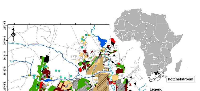
The NMDS ordinations for the open and woody grasslands showed that despite losses in
indigenous species richness the communities remained stable from 1995 to 2019 with no major changes
(Figure 2). Moreover, results of the ANOSIM analyses indicated that there were no significant changes
in species composition between the respective time periods for any of the groupings of species
(i.e., all, indigenous, exotic), for both open and woody grasslands (Table 1). Even though the woody
grassland R values were significant at p < 0.05 the values were not near 1 but near 0 which showed that
there were no real differences between the species composition of the different time periods.Sustainability 2020, 12, 1989 6 of 17
Sustainability 2020, 12, x FOR PEER REVIEW 6 of 18
Table 1. Results of the SIMPER (similarity percentages) and ANOSIM (analysis of similarity) analyses
that calculate the Bray-Curtis similarity index of the plots and whether they differ significantly for the
different time periods. p-values are significant at ≤ 0.05. Listed also is the percentage of plots where no
Woody Grasslands
exotic species were present.
All species 27 % 26 % 26 % R = 0.085 (p = 0.001)
Indigenous species SIMPER
25 % 26 % 26 % R = 0.06 (p = 0.013)
ANOSIM
(Bray-Curtis Similarity Index)
Exotic Species 45 %1995 21 2012
% 212019
% R = 0.139 (p = 0.001)
% Plots with no exotic
Open species
Grasslands 0% 8% 8%
The NMDS ordinations for the open and 26%
All species 25%
woody grasslands 22%
showed R = 0.023
that (p = 0.176)
despite losses in
Indigenous species 26% 25% 22% R = 0.023 (p = 0.186)
indigenous species richness the communities remained stable from 1995 to 2019 with no major
Exotic Species 3% 3% 6% R = 0.018 (p = 0.208)
changes (Figure 2). Moreover, results of the ANOSIM analyses indicated that there were no
% Plots with no exotic species 44% 56% 44%
significant changes in species composition between the respective time periods for any of the
Woody Grasslands
groupings ofAllspecies
species(i.e., all, indigenous, exotic),
27%for both26%
open and26% woodyRgrasslands
= 0.085 (p = (Table
0.001) 1).
Even though Indigenous
the woodyspecies
grassland R values were significant
25% at p < 0.05 26%
26% R=
the values were (p =near
0.06 not 1 but
0.013)
near 0 whichExotic
showedSpecies 45%
that there were no real differences 21%
between 21%
the R =composition
species 0.139 (p = 0.001)
of the
different time%periods.
Plots with no exotic species 0% 8% 8%
Figure
Figure 2. NMDS
2. NMDS ordination
ordination of allofspecies
all species
of theofopen
the open (a) woody
(a) and and woody grasslands
grasslands (b).outermost
(b). The The outermost
sample points of the survey period are connected to indicate the spread of
sample points of the survey period are connected to indicate the spread of the data. the data.
Analysis of the percentage occurrence of the widespread and rare indigenous and exotic species also
Analysis of the percentage occurrence of the widespread and rare indigenous and exotic species
demonstrated that proportionate distributions of these taxa stayed the same with time (Figure 3). Both
also demonstrated that proportionate distributions of these taxa stayed the same with time (Figure
the woody widespread indigenous and exotic species showed a slight increase for 2019. Open grasslands,
3). Both the woody widespread indigenous and exotic species showed a slight increase for 2019.
Openon grasslands,
the other hand, showed
on the otherahand,
slight showed
decreaseainslight
the proportion of the
decrease in widespread indigenous
proportion species.
of widespread
To determine
indigenous species. whether the suite of species remained the same, we calculated the amount of shared
and unique species found at the different time periods. In the case of the open grasslands, 66% of the
species present in 2019 were shared between 2012 and 1995, representing 51% of the original species.
Thirty-one percent of the original species were not recorded again in the resampled plots. Patterns
for the woody grasslands were similar, with 65% of the species recorded in 2019 shared between all
survey periods representing 58% of the original species with 26% unique to 1995. For both the open
and woody grasslands, some species absent in 2012 were recorded again in 2019. Indigenous species
turnover decreased dramatically from 1995–2012 to 2012–2019 in both woody and open grasslands
(Figure 4a,b). High turnover from 1995 to 2012 was a result of the disappearance of species. The rank
shift values also showed that there were a much larger reordering of species between 1995 and 2012
than between 2012 and 2019 (Figure 4c). Rank shift values of open grasslands were higher than in
woody grasslands, indicating bigger changes in community assemblages. Exotic species showed an
interesting trend where many species disappeared in open grasslands with the opposite trend in woody
grasslands for 1995–2012 (Figure 4d,e). Rank shift values were higher in both turnover periods for
woody grasslands (Figure 4f).Sustainability 2020, 12, 1989
x FOR PEER REVIEW 7 of 17
18
Figure 3. Plots indicating changes in the proportional distributions of widespread and rare indigenous
Sustainability 2020, 12, x FOR PEER REVIEW 8 of 18
and exotic species for the woody (a) and open grassland plots (b) with time.
Figure 3. Plots indicating changes in the proportional distributions of widespread and rare
indigenous and exotic species for the woody (a) and open grassland plots (b) with time.
To determine whether the suite of species remained the same, we calculated the amount of
shared and unique species found at the different time periods. In the case of the open grasslands,
66% of the species present in 2019 were shared between 2012 and 1995, representing 51% of the
original species. Thirty-one percent of the original species were not recorded again in the resampled
plots. Patterns for the woody grasslands were similar, with 65% of the species recorded in 2019
shared between all survey periods representing 58% of the original species with 26% unique to 1995.
For both the open and woody grasslands, some species absent in 2012 were recorded again in 2019.
Indigenous species turnover decreased dramatically from 1995-2012 to 2012-2019 in both woody and
open grasslands (Figures 4a,b). High turnover from 1995 to 2012 was a result of the disappearance of
species. The rank shift values also showed that there were a much larger reordering of species
between 1995 and 2012 than between 2012 and 2019 (Figure 4c). Rank shift values of open grasslands
were higher than in woody grasslands, indicating bigger changes in community assemblages. Exotic
species showed an interesting trend where many species disappeared in open grasslands with the
opposite trend in woody grasslands for 1995–2012 (Figure 4d, e). Rank shift values were higher in
both turnover periods for woody grasslands (Figure 4f).
Figure 4. Species turnover and mean rank shift analyses for open and woody grasslands. Graphs
Figure 4. Species turnover and mean rank shift analyses for open and woody grasslands. Graphs
indicate indigenous species turnover for open (a) and woody (b) grasslands, mean rank shifts for
indicate indigenous species turnover for open (a) and woody (b) grasslands, mean rank shifts for
indigenous species (c), exotic species turnover for open (d) and woody (e) grasslands, and mean rank
indigenous species (c), exotic species turnover for open (d) and woody (e) grasslands, and mean rank
shifts for exotic species (f).
shifts for exotic species (f).
3.2. Vegetation Patterns Changed Slightly between 1995 and 2019.
3.2. Vegetation Patterns Changed Slightly between 1995 and 2019.
None of the indigenous species sampled in the study area in the past or current sampling periods
were None of the
vulnerable indigenous (See
or endangered species sampled in Table
Supplementary the study
S2 for area in all
a list of theindigenous
past or current
species sampling
recorded
periods
in were
the plots andvulnerable or endangered
their conservation status).(See Supplementary
However, Table S2
species richness for a listdrastically
decreased of all indigenous
in both
species recorded in the plots and their conservation status). However, species richness decreased
drastically in both open and woody grasslands from 1995 to 2012 (see Supplementary Table S1 for a
comprehensive overview of species richness and proportionate contributions of different growth
forms, origins and life forms of all sampling periods). Total species richness remained stable from
2012 to 2019. Exotic species richness was generally low and represented 10% of the open grasslandSustainability 2020, 12, 1989 8 of 17
open and woody grasslands from 1995 to 2012 (see Supplementary Table S1 for a comprehensive
overview of species richness and proportionate contributions of different growth forms, origins and life
forms of all sampling periods). Total species richness remained stable from 2012 to 2019. Exotic species
richness was generally low and represented 10% of the open grassland species composition for all
years, with 13% (1995) and 19% (both 2012 and 2019) of the woody grasslands. Of all exotic species listed
for all time periods combined (50 species), 20 species were listed as declared invaders (Supplementary
Table S3). In keeping with the trend observed in 2012, the proportionate composition of grasses increased
and forbSustainability
species continued
2020, 12, x FORto decrease
PEER REVIEW in both the open and woody grasslands (Figure 5). 9 of 18
Figure 5. Changes
Figure in theintotal
5. Changes proportionate
the total proportionatecontribution (annual
contribution (annual andand perennial)
perennial) of different
of different growth growth
forms toforms
species composition
to species in each
composition time
in each period
time period for open(O)
for open (O)and
and woody
woody (W)(W) grasslands.
grasslands.
The biggest ‘losers’‘losers’
The biggest were indigenous forb species.
were indigenous Species
forb species. richness
Species (annual
richness andand
(annual perennial)
perennial)declined
from 104declined
in 1995from
to 70104
andin 73 respectively
1995 to 70 and 73for open grasslands
respectively with declines
for open grasslands withfrom 74 to
declines 56 74
from andto 51
56 species
in woodyandgrasslands
51 species in(Supplementary
woody grasslandsTable
(Supplementary
S1). NoneTable S1).changes
of the None of in
theperennial
changes inspecies
perennialrichness
species richness between the three sampling years were statistically significant, except for forb
between the three sampling years were statistically significant, except for forb species richness in open
species richness in open grassland habitats (Table 2).
grassland habitats (Table 2).
Table 2. ANOVA results for perennial species richness per plot between sampling years and habitats
ANOVA
Table 2.for results
indigenous for perennial
species species
richness (ISR), richness species
disturbance per plotrichness
between sampling
(DSR), years and
forb species habitats for
richness
indigenous species
(forb_SR) andrichness (ISR),
grass species disturbance
richness species
(grass_SR). richness
p-values ≤ 0.05.
(DSR),atforb
are significant species richness (forb_SR)
and grass species richness (grass_SR). p-values
One-way ANOVA
are significant at ≤ 0.05.
Post hoc Tukey Unequal N HSD
Woody ISR One-way
F(2,69) = 1.602, pANOVA
= 0.209 Post hoc
- Tukey Unequal N HSD
Woody
Woody DSR ISR F(2,69)
F(2,69) = 1.602,
= 0.688, p = 0.209
p = 0.506 - -
Woody DSR
Woody forb_SR F
F(2,79)(2,69) = 0.688, p = 0.506
= 0.889, p = 0.415 - -
Woody forb_SR F(2,79) = 0.889, p = 0.415 -
Woody grass_SR F(2,79) = 0.526, p = 0.593 -
Woody grass_SR F(2,79) = 0.526, p = 0.593 -
Grassland ISR F(2,45) = 2.840, p = 0.069 -
Grassland ISR F(2,45) = 2.840, p = 0.069 -
Grassland DSR DSR
Grassland F(2,45) = 2.987,
F(2,45) p = 0.061
= 2.987, p = 0.061 - -
Grassland forb_SR
Grassland forb_SR F(2,51) = 7.078,
F(2,51) = 7.078, p = 0.002
p = 0.002 G95 vs.G95 vsG95
G12, G12,vs.
G95 vs G19
G19
Grassland grass_SR
Grassland grass_SR F(2,51)
F(2,51) = 2.664,
= 2.664, p = 0.079
p = 0.079 - -
3.3. Time3.3. Time Lags Changed in Both Open and Woody Grassland Communities
Lags Changed in Both Open and Woody Grassland Communities
Results of the GLM analyses revealed that time lags have changed since the previous sampling
Results
periodof(Table
the GLM analyses
3). Open revealed
grassland ISR nowthat
besttime lags with
correlated havethe
changed since
2010 urban the previous
landscape sampling
measures,
period (Table 3). Open grassland ISR now best correlated with the 2010 urban landscape measures,
indicting a 9-year time lag. Open grassland DSR also indicated a 9-year time lag, which was longer
indicting a 9-year
than timesampling
for the 2012 lag. Open grassland
period DSR
but shorter also
than forindicated a 9-year
the 1995 sampling time Woody
period. lag, which was longer
grassland
plots also had changed time lags where the ISR model correlated best to the 1970 landscape,
indicating a 49-year time lag. Woody DSR patterns corresponded to a much shorter time lag periodSustainability 2020, 12, 1989 9 of 17
than for the 2012 sampling period but shorter than for the 1995 sampling period. Woody grassland
plots also had changed time lags where the ISR model correlated best to the 1970 landscape, indicating
a 49-year time lag. Woody DSR patterns corresponded to a much shorter time lag period than previous
sampling periods, now resembling the open grassland models with a 9-year time lag (Table 3).
Table 3. Simplified results of the GLM models for the three-time periods listing the landscape measures
that best explained indigenous species richness (ISR) and species richness indicative of disturbance
(DSR). Measures in bold and italics are significant at p < 0.05. The listed measures are altitude (ALT),
age of urbanization (AGE), percentage natural area (PN), road network density of natural areas (RNDN),
density of dwellings (CD) and landscape diversity (H’). The plus and minus signs indicate the direction
of the statistical relationship. For the full 1995 and 2012 table, see du Toit et al. [16] and Supplementary
Table S4 for the 2019 results.
Urban Landscape Measures Time Lag in Years
Open grassland
ISR 1995 +ALT +AGE -PN +RNDN 1
2012 +ALT +AGE +RNDN +CD +H’ 2
2019 +ALT +AGE -PN -RNDN 9
DSR 1995 -PN 25
2012 +RNDN 6
2019 -PN 9
Woody grassland
ISR 1995 -ALT -PN -RNDN -CD -H’ 25
2012 -ALT +AGE -RNDN +CD 18
2019 -CD 49
DSR 1995 -ALT -RNDN -H’ 34
2012 -ALT -PN 42
2019 PN H 9
Hanski and Ovaskainen proposed that another signature for extinction debt is the overabundance
of rare species [31]. Distribution of species occupancy histograms for perennial species only
(Supplementary Figure S1) showed that the community distributions were unimodal [64] with a
distinct peak of highest species richness of species recorded in only one site. This in itself is not a
conclusive result for overabundance as much evidence exists to indicate that a high species richness
of rare species is not unusual in ecology [64,65]. In the case of our local grasslands, due to a lack of
baseline information, we do not know if the rare species were more abundant than it ought to be.
In 1995, 27% of the species recorded were only found in one plot, this changed slightly to 26% in 2012
and 24% in 2019. However, 55% of the rare species found in 1995 were not recorded again. Of these,
forbs represented 50%. In 2012, 48% of the rare species were not recorded in 2019 of which 60% were
forbs. In 2019, 40 species were found in only one site of which 60% were forbs.
3.4. Importance of Landscape Factors Driving these Patterns Changed
The importance of the potential drivers in each model also changed for the different grassland
models (Table 3). The 2019 open grassland ISR drivers corresponded to those that were important
in 1995, but the relationship with RNDN became negative, i.e., plots with low RNDN had high ISR
patterns. The DSR model also corresponded to the same driver that was important in 1995 namely PN.
In the woody grassland models, however, the important drivers changed drastically. The ISR patterns
were now best explained by the negative relationship with the density of dwellings. In the DSR model,
the patterns now corresponded to a positive relationship with both PN and landscape diversity.
Regarding the importance of the landscape measures for the three sampling periods- in explaining
ISR patterns, both altitude (positive in open grasslands and negative in woody grasslands) and RNDN
(primarily positive) were important in five of the six models with CD important in 4 models. For DSRSustainability 2020, 12, 1989 10 of 17
patterns the most important driver was PN (primarily negative) which was important in four of the six
models (Table 3). 2020, 12, x FOR PEER REVIEW
Sustainability 11 of 18
Urban landscape measures for each of the eight time periods clearly showed how the urban
important in 4 models. For DSR patterns the most important driver was PN (primarily negative)
landscapewhich
has changed with time (Figure 6) (for the full range of measure variation for all the time
was important in four of the six models (Table 3).
periods, see Supplementary
Urban landscapeTable S5). For
measures natural
for each areas
of the eight(Figure 6a), woody
time periods clearly plots
showed hadhowconsistently
the urban higher
percentages of natural
landscape areas remaining,
has changed however,
with time (Figure 6) (foritthe
is full
clear thatofthis
range hadvariation
measure changed forconsiderably
all the time since
periods,
2010. In 2019, both seethe
Supplementary
woody andTable openS5). For naturalhad
grasslands areas (Figureaverage
similar 6a), woodyPNplots had consistently
values, with each scoring
higher percentages of natural areas remaining, however, it is clear that this had changed
53% natural areas remaining. The sharp decline in natural areas started in 1970 (Figure 6a). The density
considerably since 2010. In 2019, both the woody and open grasslands had similar average PN
of dwellings clearly
values, withshowed a rapid
each scoring 53%increase since
natural areas 1970, with
remaining. Theurban development
sharp decline in naturalincreasing
areas startedparticularly
in
in woody 1970
grassland remnants with a clear drop in the rate of urbanization in open
(Figure 6a). The density of dwellings clearly showed a rapid increase since 1970, with urban grasslands from
development increasing particularly in woody grassland remnants with
2006 onwards (Figure 6b). This indicates that most of the recent urban development encroached into a clear drop in the rate of
urbanizationThe
woody grasslands. in open
age grasslands from 2006
of urbanization onwardsthat
showed (Figure 6b). settlement
urban This indicates thattook
first mostplace
of the in open
recent urban development encroached into woody grasslands. The age of urbanization showed that
grasslandsurban
(Figure 6c). RNDN decreased drastically from 2010 to 2019 (Figure 6d), with the most
settlement first took place in open grasslands (Figure 6c). RNDN decreased drastically from
likely explanation
2010 to 2019 that more
(Figure 6d),households
with the most were supplied with
likely explanation electricity
that more householdsthan
were insupplied
the past,with which in
turn reduced the collection
electricity than in theof firewood,
past, which hence the reduced
in turn disappearance of footpaths
the collection through
of firewood, hencenatural
the areas.
Landscapedisappearance
diversity values of footpaths through
converging fornatural
the woodyareas. and
Landscape diversity values
open grasslands converging
(Figure for the results
6e) mirrored
woody and open grasslands (Figure 6e) mirrored results of the PN and CD measures, in that both
of the PN and CD measures, in that both habitats are now equally complex (multiple lands uses) with
habitats are now equally complex (multiple lands uses) with an increase in urban development in
an increasewoody
in urban development in woody grasslands.
grasslands.
Figure 6. Mean values of urban landscape measures for the eight time periods. Percentage natural
area (a), density of dwellings (b), age of urbanization (c), road network density of natural area (d),
and landscape diversity (e).Sustainability 2020, 12, 1989 11 of 17
4. Discussion
Biotic homogenization has not yet taken place in Potchefstroom, although there is clear evidence
for a steady decrease in indigenous forb species over time. Moreover, the results of the GLM models
showed that time lags in the response of vegetation patterns towards landscape drivers have changed
as well as some of the drivers responsible. This demonstrates the importance of long-term studies and
the care that should be taken with interpreting results from limited time frame research. Consequently,
it is essential to consider the history of the landscape in conservation efforts.
4.1. Little Evidence for Biotic Homogenization in Vegetation Communities from 1995 to 2019
Our results showed that, contrary to results from Melbourne [6], grasslands in the city of
Potchefstroom are not homogenizing. A few possibilities might explain this, firstly, that the intensity
of urbanization is much less than in the highly urbanized metropolitan Melbourne. In a global sense,
Potchefstroom can be seen as a small city. Secondly, Potchefstroom is also less than 200 years old
with large areas of grassland left relatively intact until major urban expansion started in 1995 [16].
Instead of homogenization, open grasslands showed slight indications of biotic differentiation (Table 1).
Percentage occurrence results indicated that the widespread indigenous species were decreasing
(Figure 3). Lastly, the lack of homogenization can be due to the low occurrence of exotic species in the
study area. Moreover, the fact that the NMDS and ANOSIM analyses showed no significant differences
between years revealed that despite high turnover and rank shifts from 1995–2012 a large suite of
widespread species did not change much.
4.2. Vegetation Patterns Changed Slightly between 1995 and 2019
The most important trend in the vegetation patterns is the proportionate composition of forb
species, especially perennials, which continually decreased with increases in graminoid species.
Moreover, the ANOVA indicated that mean forb species richness was significantly lower in open
grassland plots for both 2012 and 2019 compared to 1995. The loss of forb species, especially from
1995 to 2012, might be part of the extinction debt that is being paid. Drivers responsible for this
trend might also be linked to altered disturbance regimes of fire and grazing. When herbivores were
excluded in natural savannahs, taller fast-growing grasses shaded out lower growing forbs causing
reduced herbaceous species richness [66]. Another savannah study showed that herbivory is needed to
maintain forb species richness [67]. In Australian urban grasslands, it was also found that graminoid
species outcompeted other lower growing species, increasing their susceptibility to local extinction and
that reduced fire frequencies would potentially exacerbate the situation [32]. The interplay between
fire and grazing have been described as follows “fire affects grazing by altering large-scale foraging
patterns, and grazers affect fire by reducing fuel loads and altering fire spread in a landscape” [68].
However, in the current study, the last seven years did not indicate an acceleration in the loss of
SR but rather stable numbers with slight differences since 2012, with indigenous graminoid species,
even increasing in open grasslands (Supplementary Table S1). Decreasing numbers in indigenous
species richness in urban areas is in keeping with evidence from cities worldwide, which showed
that even though cities still contain a majority of local indigenous species it is at substantially lower
densities compared to non-urban levels [13].
Plot level differences, where some plots lost species and others gained species demonstrate that
site scale land use and management history are essential in understanding community dynamics [69].
In the current study, some plots that were degraded in 2012 improved in 2019 due to lower human
impacts as represented by the reduction in RNDN values in 2019. However, the presence of time lags
and the significant loss of indigenous forb richness indicated that despite slight increases in species
richness, the evidence for extinction debts reveals that the situation will not improve but will exacerbate
in the future if nothing is done about the situation. In their paper on the global synthesis of plant
extinction rates in urban areas, Hahs et al. divided cities into three types based on their landscapeSustainability 2020, 12, 1989 12 of 17
transformation history, namely cities highly transformed before 1600 AD, those transformed after
1600 AD but before initial floristic surveys were carried out, and those where initial surveys were
done before extensive transformation, i.e., intact native vegetation existed during the surveys [29].
Potchefstroom falls into the third category and is, therefore, likely to carry extinction debts due to
the difference in species still present and the predicted species richness based on available habitat.
Consequently, development was recent enough for native vegetation to still largely persists in remnant
patches. However, without conservation efforts, the authors argue that these populations will not be
viable in the long term [29].
4.3. Time Lags Changed in Both Open and Woody Grassland Communities
Our GLM analyses showed that the time lags for open grasslands have changed to a 9 year
lag for both the ISR and DSR patterns. In terms of the ISR patterns, this could mean that critical
habitat loss due to development and fragmentation had been reached in 2010. This might indicate that
habitat quality declined to a critical level due to anthropogenic influences [70], loss of grazing or fire
suppression. Moreover, due to the known poor seedbank of grassland species [71], the seedbank might
be depleted. The similarity of the DSR time lags to that of the open grassland ISR patterns could also
indicate that DSR species responded to the same critical threshold as that of the native grassland species.
In our previous paper, we hypothesized that the DSR time lags could act as early warning signals [16],
the current results reveal that due to the potential critical threshold reached, this seems no longer to be
true. Time lags of the woody grassland ISR were still longer than open grassland species, however,
the best fit model now showed that time lags were much longer than initially recorded. A possible
explanation for these changes might be found in a recent editorial in response to an intense debate on
the effects of fragmentation on biodiversity [72]. The authors highlighted a few key points in the debate
that included the importance of the temporal scale. They argued that “more habitat fragmentation
might result in greater initial changes in some populations and later changes in others. We cannot
assume that the initial rates of biodiversity change observed at different levels of fragmentation will
remain over longer time periods” [72]. Another factor to consider in explaining changing time lags is
the changes in community equilibrium as habitats change in relation to extinction thresholds [31] and
as the extinction debt is paid out [26].
More research on global plant extinctions in urban areas should be undertaken because
comprehensive surveys exist of historic and recent floral composition in these urban areas [29].
The changing time lags for the three sampling periods demonstrate that we should be careful in
interpreting the results of a single survey. Continuous monitoring is essential to understand the
underlying patterns and processes. Our study revealed that the history of the landscape affects current
vegetation communities and conservationists need to account for history in contemporary observed
patterns in nature.
4.4. The Importance of Landscape Factors Driving these Patterns Changed
Our results showed that the importance of some of the landscape measures and the direction of
the relationships changed between sampling years. This has important ramifications for selecting and
using landscape measures in quantifying time lags as well as incorporating the changing dynamics
of the strength of drivers that can change over time in the same landscape. Moreover, this again
highlights the importance of long-term studies to monitor changes in the landscape. If we want to
aid policymakers and conservationists in effectively managing urban vegetation, decision-makers
need to know which drivers are responsible for vegetation composition and patterns. However, we
acknowledge that drivers we did not include here could potentially be important in explaining the
observed patterns. Two such important drivers are grazing and fire as discussed earlier in explaining
the changes in vegetation patterns.Sustainability 2020, 12, 1989 13 of 17
4.5. Consequently, How will the Presence of Time Lags and Potential Extinction Debts Influence Conservation
Strategies and Planning for Resilient and Sustainable Cities?
In Potchefstroom, biotic homogenization has not yet taken place which means that here remnant
natural urban vegetation is still worthy of conservation. However, evidence of a significant decrease in
forb species richness combined with the calculated time lags reveal that even in Potchefstroom, with no
visible biotic homogenization, keeping the conservation and management status quo is not enough.
Pro-active management and restoration are essential to ensure the long-term sustainability of grassland
diversity. Better management of extant vegetation and the restoration of native vegetation in the
landscape can reduce the extinction debt [25,29]. In grasslands the best restoration results were with
planting seedlings in disturbed sites, moreover, exotic weed density was also limited by successfully
established native species [73]. Other studies showed that success depends on the re-establishment
of swards of the correct indigenous perennial grass species [74]. The removal of dominant grass
species allows light availability for intertussock forbs [75,76], however, in their study in Australian
grasslands Johnson et al. found that seed limitation of forbs was a constraint to the recovery of
degraded grasslands as indigenous forb recruitment mostly relied upon seed addition [76]. This
finding is also supported by Zamin et al. [77]. Another management strategy that could be employed
in fragmented natural areas is the collection of forb seeds from nearby natural areas and sowing it
in degraded urban open spaces including along road verges and railway embankments [78]. Such
a strategy could have several benefits in terms of improving the environment, recovering degraded
areas with native vegetation, increasing biodiversity, creating “ecological continuity” between the
inner city and surrounding natural areas, decreasing maintenance, and also increasing awareness and
involvement amongst city residents in terms of the importance of protecting native grasslands [78].
However, not all researchers agree that seeding is the best strategy. In dryland ecosystems, seeding
often fails because managers do not account for seed dormancy and germination traits [79]. Whereas,
in neotropical grasslands, the translocation of topsoil and transplantation of mature forbs and grasses
proved to be the most successful restoration technique [80].
Volis and Deng contend that population demographic assessments should be the first step in any
conservation project to determine population viability and appropriate population management [81].
Time lags in the response of species to disturbances can obscure the true conservation status of plants [81].
Our study also revealed that drivers previously associated with vegetation patterns changed. This
means that revisitation and long-term studies are essential to understand vegetation dynamics and
to continuously ensure that the correct drivers are managed and planned for. Moreover, researchers
should be careful to attribute causation too readily to drivers gleaned from limited time frame studies,
emphasizing the importance of continuous monitoring. As early as 1990, Magnuson pleaded that
“in the absence of the temporal context provided by long-term research, serious misjudgments can
occur not only in our attempts to understand and predict a change in the world around us but also in
our attempts to manage our environment.” [21]. Future measures require the mobilization of efforts
well beyond current investment in conservation and need to account for both new and old drivers and
possible extinction debts.
Supplementary Materials: The following are available online at http://www.mdpi.com/2071-1050/12/5/1989/s1,
Table S1: Species richness and percentage contributions (annual and perennial) for all comparable sites between
the sampling periods (sites that could not be resampled in 2019 were excluded from previous surveys). Table S2:
List of all the indigenous species recorded in the comparison sites for all sampling periods. The list includes
the conservation status based on the Red List of South African Plants [82] and the number of plots in which the
species occurred for each habitat type and sampling period. The bold text and dark grey fill indicate widespread
species and the light grey rare species based on Gaston’s Quartile Criterion [61]. Plant names according to the Red
List [82] and Germishuizen et al. [83]. Table S3: List of all the exotic species recorded in the comparison sites for all
sampling periods. The list includes the invasive status based on the Conservation of Agricultural Resources Act,
1983 (Act No 43 of 1983) (CARA) amended in 2001 and the National Environmental Management: Biodiversity
Act (10/2004) (NEMBA): Draft Alien and Invasive Species Lists, 2014 categories. Listed also is the number of
plots in which the species occurred for each habitat type and sampling period. The bold text and dark grey fill
indicate widespread species and the light grey rare species based on Gaston’s Quartile Criterion [61]. Plant names
according to Germishuizen et al. [83]. Table S4: Results of the GLM model for 2019. Model coefficients (±SE)Sustainability 2020, 12, 1989 14 of 17
are presented, as well as p values. Model intercept (Int), altitude (ALT), age of urbanization (AGE), percentage
natural area (PN), road network density of natural areas (RNDN), density of dwellings (CD), Shannon’s diversity
index of landscape diversity (H’). Akaike’s information criterion (AIC) for the model with the highest AIC value
(and year), and the model with the lowest AIC (and year, in bold). GLM model coefficients and SE and p values
presented here are from models with the lowest AIC values. L2 and L3 represent the second and third levels of a
variable classified as a factor. Table S5: List of the range of variation for each calculated urban landscape measure
for all time periods. The listed measures are altitude (ALT), age of urbanization (AGE), percentage natural area
(PN), road network density of natural areas (RNDN), density of dwellings (CD) and landscape diversity (H’),
Figure S1: Distribution of species occupancy histograms for open and woody grasslands for all sampling periods
indicating unimodal distributions.
Author Contributions: Conceptualization, M.J.d.T. and S.S.C.; Data curation, M.J.d.T. and D.J.K.; Formal
analysis, M.J.d.T. and D.J.K.; Investigation, M.J.d.T. and S.S.C.; Methodology, M.J.d.T., S.S.C. and D.J.K.; Project
administration, M.J.d.T.; Resources, S.S.C. and D.J.K.; Software, D.J.K.; Supervision, M.J.d.T. and S.S.C.; Validation,
S.S.C. and D.J.K.; Visualization, M.J.d.T.; Writing—original draft, M.J.d.T., S.S.C. and D.J.K.; Writing—review
& editing, M.J.d.T., S.S.C. and D.J.K. All authors have read and agreed to the published version of the manuscript.
Funding: SC acknowledges the NRF for financial support for fieldwork.
Conflicts of Interest: The authors declare no conflict of interest.
References
1. Aronson, M.F.J.; Nilon, C.H.; Lepczyk, C.A.; Parker, T.S.; Warren, P.S.; Cilliers, S.S.; Goddard, M.A.; Hahs, A.K.;
Herzog, C.; Katti, M.; et al. Hierarchical filters determine community assembly of urban species pools.
Ecology 2016, 97, 2952–2963. [CrossRef] [PubMed]
2. Kowarik, I. Novel urban ecosystems, biodiversity, and conservation. Environ. Pollut. 2011, 159, 1974–1983.
[CrossRef] [PubMed]
3. McKinney, M.L. Effects of urbanization on species richness: A review of plants and animals. Urban Ecosyst.
2008, 11, 161–176. [CrossRef]
4. Olden, J.D. Biotic homogenization: A new research agenda for conservation biogeography. J. Biogeogr. 2006,
33, 2027–2039. [CrossRef]
5. McKinney, M.L. Urbanization as a major cause of biotic homogenization. Biol. Conserv. 2006, 127, 247–260.
[CrossRef]
6. Zeeman, B.J.; McDonnell, M.J.; Kendal, D.; Morgan, J.W.; Schmidtlein, S. Biotic homogenization in an
increasingly urbanized temperate grassland ecosystem. J. Veg. Sci. 2017, 28, 550–561. [CrossRef]
7. Blouin, D.; Pellerin, S.; Poulin, M. Increase in non-native species richness leads to biotic homogenization in
vacant lots of a highly urbanized landscape. Urban Ecosyst. 2019, 22, 879–892. [CrossRef]
8. Olden, J.D.; Poff, N.L. Toward a mechanistic understanding and prediction of biotic homogenization. Am. Nat.
2003, 162, 442–460. [CrossRef]
9. Lososová, Z.; Chytrý, M.; Tichý, L.; Danihelka, J.; Fajmon, K.; Hájek, O.; Kintrová, K.; Láníková, D.;
Otýpková, Z.; Řehořek, V. Biotic homogenization of central european urban floras depends on residence
time of alien species and habitat types. Biol. Conserv. 2012, 145, 179–184. [CrossRef]
10. La Sorte, F.A.; Aronson, M.F.J.; Williams, N.S.G.; Celesti-Grapow, L.; Cilliers, S.; Clarkson, B.D.; Dolan, R.W.;
Hipp, A.; Klotz, S.; Kühn, I.; et al. Beta diversity of urban floras among European and non-European cities.
Global Ecol. Biogeogr. 2014, 23, 769–779. [CrossRef]
11. Lososová, Z.; Chytrý, M.; Danihelka, J.; Tichý, L.; Ricotta, C.; Kühn, I. Biotic homogenization of urban
floras by alien species: The role of species turnover and richness differences. J. Veg. Sci. 2016, 27, 452–459.
[CrossRef]
12. Miller, J.R. Biodiversity conservation and the extinction of experience. Trends Ecol. Evol. 2005, 20, 430–434.
[CrossRef] [PubMed]
13. Aronson, M.F.; La Sorte, F.A.; Nilon, C.H.; Katti, M.; Goddard, M.A.; Lepczyk, C.A.; Warren, P.S.; Williams, N.S.;
Cilliers, S.; Clarkson, B.; et al. A global analysis of the impacts of urbanization on bird and plant diversity
reveals key anthropogenic drivers. Proc. Biol. Sci. 2014, 281, 20133330. [CrossRef] [PubMed]
14. Rhemtulla, J.M.; Mladenoff, D.J. Why history matters in landscape ecology. Landsc. Ecol. 2007, 22, 1–3.
[CrossRef]
15. Ramalho, C.E.; Hobbs, R.J. Time for a change: Dynamic urban ecology. Trends Ecol. Evol. 2012, 27, 179–188.
[CrossRef]You can also read