Space-Time Completion of Video - Yonatan Wexler, Member, IEEE Computer Society, Eli Shechtman, Student Member, IEEE Computer Society, and Michal ...
←
→
Page content transcription
If your browser does not render page correctly, please read the page content below
IEEE TRANSACTIONS ON PATTERN ANALYSIS AND MACHINE INTELLIGENCE,                        VOL. 29, NO. 3,      MARCH 2007                              1

                       Space-Time Completion of Video
                                   Yonatan Wexler, Member, IEEE Computer Society,
                             Eli Shechtman, Student Member, IEEE Computer Society, and
                                     Michal Irani, Member, IEEE Computer Society

       Abstract—This paper presents a new framework for the completion of missing information based on local structures. It poses the task
       of completion as a global optimization problem with a well-defined objective function and derives a new algorithm to optimize it. Missing
       values are constrained to form coherent structures with respect to reference examples. We apply this method to space-time completion
       of large space-time “holes” in video sequences of complex dynamic scenes. The missing portions are filled in by sampling spatio-
       temporal patches from the available parts of the video, while enforcing global spatio-temporal consistency between all patches in and
       around the hole. The consistent completion of static scene parts simultaneously with dynamic behaviors leads to realistic looking video
       sequences and images. Space-time video completion is useful for a variety of tasks, including, but not limited to: 1) Sophisticated video
       removal (of undesired static or dynamic objects) by completing the appropriate static or dynamic background information. 2) Correction
       of missing/corrupted video frames in old movies. 3) Modifying a visual story by replacing unwanted elements. 4) Creation of video
       textures by extending smaller ones. 5) Creation of complete field-of-view stabilized video. 6) As images are one-frame videos, we
       apply the method to this special case as well.

       Index Terms—Video analysis, texture, space-time analysis.

                                                                                 Ç

1    INTRODUCTION

W      E present a method for space-time completion of large
       space-time “holes” in video sequences of complex
dynamic scenes. We follow the spirit of [14] and use non-
                                                                                         Fig. 1 shows an example of the task at hand. Given the input
                                                                                     video (Fig. 1a), a space-time hole is specified in the sequence
                                                                                     (Fig. 1b). The algorithm is requested to complete this hole
parametric sampling, while extending it to handle static and                         using information from the remainder of the sequence. We
dynamic information simultaneously. The missing video                                assume that the hole is provided to the algorithm. While in all
                                                                                     examples here it was marked manually, it can also be the
portions are filled in by sampling spatio-temporal patches
                                                                                     outcome of some segmentation algorithm. The resulting
from other video portions, while enforcing global spatio-
                                                                                     completion and the output sequence are shown in Fig. 1c.
temporal consistency between all patches in and around the                               The goal of this work is close to a few well-studied
hole. Global consistency is obtained by posing the problem of                        domains. Texture Synthesis (e.g., [2], [14], [28]) extends and
video completion/synthesis as a global optimization pro-                             fills regular fronto-parallel image textures. This is similar to
blem with a well-defined objective function and solving it                           Image Completion (e.g., [9], [12]) which aims at filling in large
appropriately. The objective function states that the resulting                      missing image portions. While impressive results have been
completion should satisfy the following two constraints:                             achieved recently in some very challenging cases (e.g., see
1) Every local space-time patch of the video sequence should                         [12]), the goal and the proposed algorithms have so far been
be similar to some local space-time patch in the remaining                           defined only in a heuristic way. Global inconsistencies often
parts of the video sequence (the “input data set”), while                            result from independent local decisions taken at indepen-
2) globally all these patches must be consistent with each other,                    dent image positions. For this reason, these algorithms use
both spatially and temporally.                                                       large image patches in order to increase the chances of
    Solving the above optimization problem is not a simple                           correct output. The two drawbacks of this approach are that
                                                                                     elaborate methods for combining the large patches are
task, especially due to the large dimensionality of video data.
                                                                                     needed for hiding inconsistencies [12], [13], [21], and that
However, we exploit the spatio-temporal relations and
                                                                                     the data set needs to be artificially enlarged by including
redundancies to speed and constrain the optimization process                         various skewed and scaled replicas that might be needed
in order to obtain realistic looking video sequences with                            for completion. When compared to the pioneering work of
complex scene dynamics at reasonable computation times.                              [14] and its derivatives, the algorithm presented here can be
                                                                                     viewed as stating an objective function explicitly. From this
                                                                                     angle, the algorithm of [14] makes a greedy decision in each
. Y. Wexler is with Microsoft, 1 Microsoft Way, Redmond, WA 98052.
  E-mail: yonatan.wexler@microsoft.com.
                                                                                     pixel based on the currently available pixels around it. It
. E. Shechtman and M. Irani are with the Department of Computer Science              only uses a directional neighborhood around each pixel. A
  and Applied Math, Ziskind Building, The Weizmann Institute of Science,             greedy approach requires the correct decision to be made at
  Rehovot, 76100 Israel.                                                             every step. Hence, the chances for errors increase rapidly as
  E-mail: {eli.shechtman, michal.irani}@weizmann.ac.il.
                                                                                     the gap grows. The work of [9] showed that this may be
Manuscript received 19 July 2005; revised 15 Jan. 2006; accepted 27 June             alleviated by prioritizing the completion order using local
2006; published online 15 Jan. 2007.
Recommended for acceptance by P. Torr.
                                                                                     image structure. In challenging cases containing complex
For information on obtaining reprints of this article, please send e-mail to:        scenes and large gaps, the local neighborhood does not hold
tpami@computer.org, and reference IEEECS Log Number TPAMI-0382-0705.                 enough information for a globally correct solution. This is
                                               0162-8828/07/$20.00 ß 2007 IEEE       Published by the IEEE Computer Society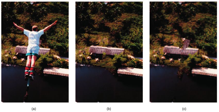
2                                      IEEE TRANSACTIONS ON PATTERN ANALYSIS AND MACHINE INTELLIGENCE,                VOL. 29,   NO. 3,   MARCH 2007

Fig. 1. 1) Few frames out of a video sequence showing one person standing and waving her hands while the other person is hopping behind her. The
video size is 100  300  240, with 97,520 missing pixels. 2) A zoomed-in view on a portion of the video around the space-time hole before and after
the completion. Note that the recovered arms of the hopping person are at slightly different orientations than the removed ones. As this particular
instance does not exist anywhere else in the sequence, a similar one from a different time instance was chosen to provide an equally likely
completion. See video at: http://www.wisdom.weizmann.ac.il/~vision/VideoCompletion.html. (a) Input Sequence. (b) Occluder cut out manually.
(c) Spatio-temporal completion.

Fig. 2. Sources of information. Output frame 114, shown in (a), is a combination of the patches marked here in red over the input sequence (c). It is
noticeable that large continuous regions have been automatically picked whenever possible. Note that the hair, head, and body were taken from
different frames. The original frame is shown in (b). (a) Output. (b) Input. (c) Selected patches.

more pronounced in video. Due to motion aliasing, there is                     Image Inpainting (e.g., [5], [6], [22]) was defined in a
little chance that an exact match will be found.                            principled way as an edge continuation process, but is
    The framework presented here requires that the whole                    restricted to small (narrow) missing image portions in
neighborhood around each pixel is considered, not just a                    highly structured image data. These approaches have been
                                                                            restricted to the completion of spatial information alone in
causal subset of it. Moreover, it considers all windows                     images. Even when applied to video sequences (as in [4]),
containing each pixel simultaneously, thus effectively using                the completion was still performed spatially. The temporal
an even larger neighborhood.                                                component of video has mostly been ignored. The basic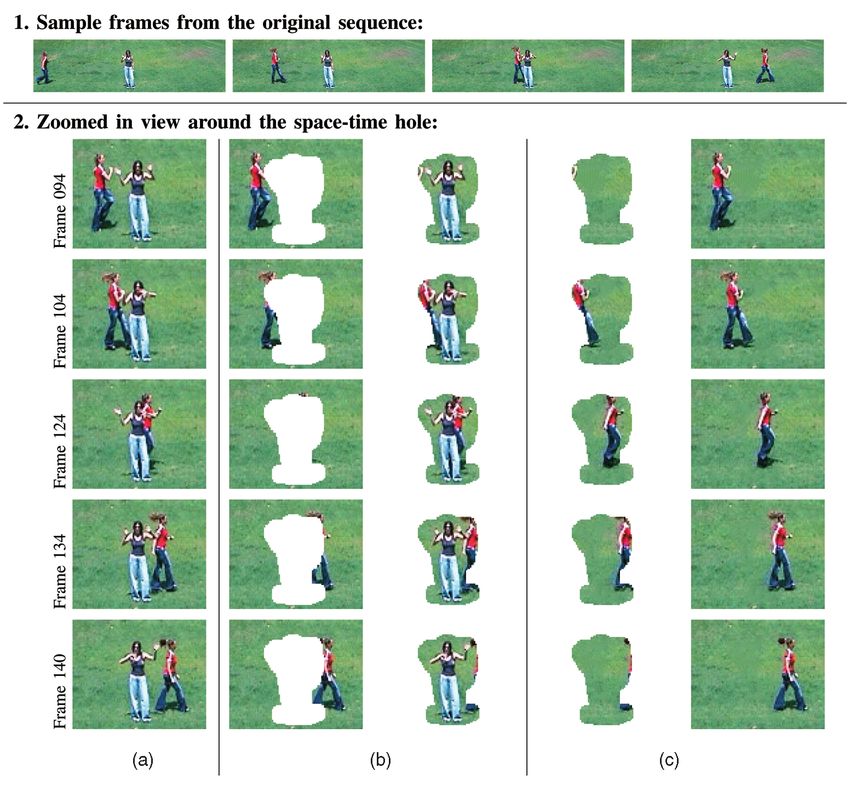
WEXLER ET AL.: SPACE-TIME COMPLETION OF VIDEO                                                                                        3

assumption of Image Inpainting, that edges should be                   The approach presented here can automatically handle
interpolated in some smooth way, does not naturally extend          the completion and synthesis of both structured dynamic
to time. Temporal aliasing is typically much stronger than          objects as well as unstructured dynamic objects under a
spatial aliasing in video sequences of dynamic scenes.              single framework. It can complete frames (or portions of
Often, a pixel may contain background information in one            them) that never existed in the data set. Such frames are
frame and foreground information in the next frame,                 constructed from various space-time patches, which are
resulting in very nonsmooth temporal changes. These                 automatically selected from different parts of the video
violate the underlying assumptions of Inpainting.                   sequence, all put together consistently. The use of a global
   In [19], a method has been proposed for employing spatio-        objective function removes the pitfalls of local inconsisten-
temporal information to correct scratches and noise in poor-        cies and the heuristics of using large patches. As can be seen
quality video sequences. This approach relies on optical-flow       in the figures and in the attached videos, the method is
estimation and propagation into the missing parts followed          capable of completing large space-time areas of missing
by reconstruction of the color data. The method was extended        information containing complex structured dynamic scenes,
to removal of large objects in [20] under the assumption of         just as it can work on complex images. Moreover, this
planar rigid layers and small camera motions.                       method provides a unified framework for various types of
   View Synthesis deals with computing the appearance of a          image and video completion and synthesis tasks, with the
scene from a new viewpoint, given several images. A                 appropriate choice of the spatial and temporal extents of the
similar objective was already used in [15] for successfully         space-time “hole” and of the space-time patches. A
resolving ambiguities which are otherwise inherent to the           preliminary version of this work appeared in CVPR ’04 [29].
geometric problem of new-view synthesis from multiple                  This paper is organized as follows: Section 2 introduces
camera views. The objective function of [15] was defined on         the objective function and Section 3 describes the algorithm
2D images. Their local distance between 2D patches was              used for optimizing it. Sections 4 and 5 discuss trade-offs
based on SSD of color information and included geometric            between space and time dimensions in video and how they
constraints. The algorithm there did not take into account          are unified into one framework. Section 6 demonstrates the
the dependencies between neighboring pixels as only the             application of this method to various problems. Finally,
central point was updated in each step.                             Section 7 concludes this paper.
   Recently, there have been a few notable approaches to
video completion. From the algorithmic perspective, the most        2   COMPLETION        AS A   GLOBAL OPTIMIZATION
similar work to ours is [7], which learns a mapping from the
input video into a smaller volume, aptly called “epitome.”          Given a video sequence, we wish to complete the missing
These are then used for various tasks including completion.         portions in such a way that it looks just like the available parts.
While our work has a similar formulation, there are major           For this, we define a global objective function to rank the
differences. We seek some cover of the missing data by the          quality of a completion. Such a function needs to take a
available information. Some regions may contribute more             completed video and rate its quality with respect to a reference
than once while some may not contribute at all. In contrast,        one. Its extremum should denote the best possible solution.
the epitome contains a proportional representation of all the          Our basic observation is that, in order for a video to
data. One implication of this is that the windows will be           look good, it needs to be coherent everywhere. That is, a
averaged and, so, will lose some fidelity. The recent work of       good completion should resemble the given data locally
[24] uses estimated optical flow to separate foreground and         everywhere.
background layers. Each is then filled incrementally using the         The constraint on the color of each pixel depends on the
priority-based ordering idea similar to [9].                        joint color assignment of its neighbors. This induces a
   Finally, the work of [18] takes an object-based approach         structure where each pixel depends on the neighboring ones.
where large portions of the video are tracked, their cycles         The correctness of a pixel value depends on whether its local
are analyzed, and they can then be inserted into the video.         neighborhood forms a coherent structure. Rather than
This allows warping of the object so it fits better, but            modeling this structure, we follow [14] and use the reference
requires a complete appearance of the object to be identified       video as a library of video samples that are considered to be
and, so, is not applicable to more complex dynamics, such           coherent.
as articulated motion or stochastic textures.                          Given these guidelines, we are now ready to describe our
   A closely related area of research which regards temporal        framework in detail.
information explicitly is that of dynamic texture synthesis in
videos (e.g., [3], [11]). Dynamic textures are usually character-   2.1 The Global Objective Function
ized by an unstructured stochastic process. They model and          To allow for a uniform treatment of dynamic and static
synthesize smoke, water, fire, etc., but cannot model nor           information, we treat video sequences as space-time
synthesize structured dynamic objects, such as behaving             volumes. We use the following notations: A pixel ðx; yÞ in a
people. We demonstrate the use of our method for synthesiz-         frame t will be regarded as a space-time point p ¼ ðx; y; tÞ in
ing large video textures from small ones in Section 6. While        the volume. Wp denotes a small, fixed-sized window around
[26] has been able to synthesize/complete video frames of           the point p both in space and in time. The diameter of the
structured dynamic scenes, it assumes that the “missing”            window is given as a parameter. We use indices i and j to
frames already appear in their entirety elsewhere in the input      denote locations relative to p. For example, Wp is the window
video and, therefore, needed only to identify the correct           centered around p and Wpi is the ith window containing p
permutation of frames. An extension of that paper [25]              and is centered around the ith neighbor of p.
manually composed smaller “video sprites” to a new                     We say that a video sequence S has global visual coherence
sequence.                                                           with some other sequence D if every local space-time patch in
4                                          IEEE TRANSACTIONS ON PATTERN ANALYSIS AND MACHINE INTELLIGENCE,            VOL. 29,   NO. 3,   MARCH 2007

Fig. 3. Local and global space-time consistency. (a) Enforcement of the global objective function of (1) requires coherence of all space-time patches
containing the point p. (b) Such coherence leads to a globally correct solution. The true trajectory of the moving object is marked in red and is
correctly recovered. When only local constraints are used and no global consistency enforced, the resulting completion leads to inconsistencies (c).
The background figure is wrongly recovered twice with wrong motion trajectories.

S can be found somewhere within the sequence D. In other                    Fig. 3c. A greedy approach requires the correct answer to be
words, we can cover S with small windows from D. Windows                    found at every step and this is rarely the case as local image
in the data set D are denoted by V and are indexed by a                     structure will often contain ambiguous information.
reference pixel (e.g., Vq and Vqi ).                                           The above objective function seeks a cover of the missing
   Let S and H  S be an input sequence and a “hole” region                 data using the available one. That is, among the exponen-
within it. That is, H denotes all the missing space-time points             tially large number of possible covers, we seek the one that
within S. For example, H can be an undesired object to be                   will give us the least amount of total error. The motivation
erased, a scratch or noise in old corrupt footage, or entire                here is to find a solution that is correct everywhere, as any
missing frames, etc. We assume that both S and H are given.                 local inconsistency will push the solution away from the
   We wish to complete the missing space-time region H with                 minimum.
some new data H such that the resulting video sequence S                  2.2 The Local Space-Time Similarity Measure
will have as much global visual coherence with some
                                                                            At the heart of the algorithm is a well-suited similarity
reference sequence D (the data set). Typically, D ¼ S n H,
                                                                            measure between space-time patches. A good measure
namely, the remaining video portions outside the hole, are
                                                                            needs to agree perceptually with a human observer. The Sum
used to fill in the hole. Therefore, we seek a sequence S  which
                                                                            of Squared Differences (SSD) of color information, which is
maximizes the following objective function:
                                                                            so widely used for image completion, does not suffice for
                                 Y                                          the desired results in video (regardless of the choice of color
           CoherenceðS  jDÞ ¼        max simðWp ; Vq Þ;      ð1Þ
                                   p2S
                                           q2D                              space). The main reason for this is that the human eye is
                                                                            very sensitive to motion. Maintaining motion continuity is
where p, q run over all space-time points in their respective               more important than finding the exact spatial pattern match
sequences. simð; Þ is a local similarity measure between                  within an image of the video.
two space-time patches that will be defined shortly                            Fig. 4 illustrates (in 1D) that very different temporal
(Section 2.2). The patches need not necessarily be isotropic                behaviors can lead to the same SSD score. The function fðtÞ
and can have different sizes in the spatial and temporal                    has a noticeable temporal change. Yet, its SSD score relative
dimensions. We typically use 5  5  5 patches which are                    to a similar looking function g1 ðtÞRis the same as the
                                                                                                                                 R SSD score
large enough to be statistically meaningful but small                       of fðtÞ with a flat function g2 ðtÞ: ðf  g1 Þ2 dt ¼ ðf  g2 Þ2 dt.
enough so that effects, such as parallax or small rotations,                However, perceptually, fðtÞ and g1 ðtÞ are more similar, as
will not affect them. They are the basic building blocks of                 they both encode a temporal change.
the algorithm. The use of windows with temporal extent                         We would like to incorporate this into our algorithm so
assumes that the patches are correlated in time, and not                    to create a similarity measure that agrees with perceptual
only in space. When the camera is static or fully stabilized,               similarity. Therefore, we add a measure that is similar to
this is trivially true. However, it may also apply in other                 that of normal-flow to obtain a quick and rough approx-
cases where the same camera motion appears in the                           imation of the motion information. Let Y be the sequence
database (as shown in Fig. 16).                                             containing the grayscale (intensity) information obtained
   Fig. 3 explains why (1) induces global coherence. Each                   from the color sequence. At each space-time point, we
space-time point p belongs to other space-time patches of                   compute the spatial and temporal derivatives ðYx ; Yy ; Yt Þ. If
other space-time points in its vicinity. For example, for a                 the motion were only horizontal, then u ¼ Yt =Yx would
5  5  5 window, 125 different patches involve p. The red
                                                                            capture the instantaneous motion in the x direction. If the
and green boxes in Fig. 3a are examples of two such
patches. Equation (1) requires that all 125 patches agree on
the value of p and, therefore, (1) leads to globally coherent
completions such as the one in Fig. 3b. If the global
coherence of (1) is not enforced, and the value of p is
determined locally by a single best-matching patch (i.e.,
using a sequential greedy algorithm as in [9], [14], [24]),
then global inconsistencies will occur in a later stage of the
recovery. An example of temporal incoherence is shown in                    Fig. 4. Importance of matching derivatives (see text).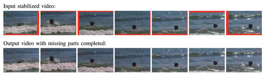
WEXLER ET AL.: SPACE-TIME COMPLETION OF VIDEO                                                                                         5

Fig. 5. Video completion algorithm.

motion were only vertical, then v ¼ Yt =Yy would capture the                                     9V i 2 D; Wpi ¼ V i :
instantaneous motion in the y direction. The fractions factor              2.   All those V 1 . . . V k agree on the color value c at
out most of the dependence between the spatial and                              location p:
the temporal changes (such as frame-rate) while capturing
object velocities and directions. These two components                                            c ¼ V i ðpÞ ¼ V j ðpÞ:
are scaled and added to the RGB measurements to obtain
                                                                        This is trivially true since the second condition is a
a five-dimensional representation for each space-time point:
                                                                        particular case of the first. These conditions imply an
ðR; G; B; u; vÞ, where  ¼ 5. Note that we do not compute             iterative algorithm. The iterative step will aim at satisfying
optical flow. We apply an L2 -norm (SSD) to this                        these two conditions locally at every point p. Any change in
5D representation in order to capture space-time similarities           p will affect all the windows that contain it and, so, the
for static and dynamic parts simultaneously. Namely, for                update rule must take all of them into account.
two space-time windows Wp and Vq , we have dðWp ; Vq Þ ¼                   Note that (1) may have an almost trivial solution in which
P                                       2
   ðx;y;tÞ kWp ðx; y; tÞ  Vq ðx; y; tÞk , where, for each ðx; y; tÞ
                                                                        the hole H contains an exact copy of some part in the
within the patch, Wp ðx; y; tÞ denotes its 5D measurement               database. For such a solution, the error inside the hole will
vector. The distance is translated to the similarity measure            be zero (as both conditions above are satisfied) and, so, the
                                                                        total coherence error will be proportional to the surface area
                                              dðWp ;Vq Þ
                                                                        of the space-time boundary. This error might be much
                      simðWp ; Vq Þ ¼ e        22        :      ð2Þ
                                                                        smaller than small noise errors spread across the entire
The choice of  is important as it controls the smoothness of           volume of the hole. Therefore, we associate an additional
the induced error surface. Rather than using a fixed value, it          quantity p to each point p 2 S. Known points p 2 S n H
is chosen to be the 75-percentile of all distances in the               have fixed high confidence, whereas missing points p 2 H
current search in all locations. In this way, the majority of           will have lower confidence. This weight is chosen so to
locations are taken into account and, hence, there is a high            ensure that the total error inside the hole is less than that on
probability that the overall error will reduce.                         the hole boundary. This argument needs to hold recursively
                                                                        in every layer in the hole. An approximation to such
                                                                        weighting is to compute the distance transform for every
3    THE OPTIMIZATION                                                   hole pixel and then use p ¼  dist . When the hole is roughly
The inputs to the optimization are a sequence S and a                   spherical, choosing  ¼ 1:3 gives the desired weighting. This
“hole” H  S, marking the missing space-time points to be               measure bears some similarity to the priority used in [9]
corrected or filled in. The algorithm seeks an assignment of            except that, here, it is fixed throughout the process. Another
color values for all the space-time points (pixels) in the hole         motivation for using such weighting is to speed up
so to satisfy (1). While (1) does not imply any optimization            convergence by directing the flow of information inward
scheme, we note that it will be satisfied if the following two          from the boundary.
local conditions are met at every space-time point p:                   3.1 The Iterative Step
    1.   All windows     Wp1   . . . Wpk   containing p appear in the   Let p 2 H be some hole point which we wish to improve.
         data set D:                                                    Let Wp1 . . . Wpk be all space-time patches containing p. Let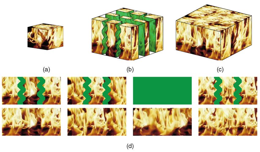
6                                       IEEE TRANSACTIONS ON PATTERN ANALYSIS AND MACHINE INTELLIGENCE,                 VOL. 29,   NO. 3,   MARCH 2007

Fig. 6. Multiscale solution. The algorithm starts by shrinking the input video (both in space and in time). The completion starts at the coarsest level,
iterating each level several times and propagating the result upward.
                                                                                                           P      i i
V 1 . . . V k denote the patches in D that are most similar                                                  i2M !p c
                                                                                                         c¼ P      i
                                                                                                                      :                             ð4Þ
to Wp1 . . . Wpk per (2). According to Condition 1 above, if Wpi                                              i2M !p

is reliable, then dðWpi ; V i Þ  0. Therefore, simðWpi ; V i Þ              This update rule produces a robust estimate for the pixel in the
measures the degree of reliability of the patch Wpi .                        presence of noise. While making the algorithm slightly more
    We need to pick a color c at location p so that the coherence            complex, this step has further advantages. The bandwidth
at all windows containing it will increase. Each window V i                  parameter controls the degree of smoothness of the error
provides an evidence of possible solution for c and the                      surface. When it is large, it reduces to simple weighted
confidence in this evidence is given by (2) as sip ¼ simðWpi ; V i Þ.        averaging (as in (3)), hence allowing rapid convergence.
According to Condition 2 above, the most likely color c at p                 When it is small, it induces a weighted majority vote, avoiding
                                                                             blurring in the resulting output. The use of a varying  value
should minimize the variance of the colors c1 . . . ck proposed
                                                                             has significantly improved the convergence of the algorithm.
by V 1 . . . V k at location p. As mentioned before, these values            When compared with the original work in [29], the results
should be scaled according to the fixed ip to avoid the trivial             shown here achieve better convergence. This can be seen from
solution. Thus, the most likely color at p will minimize                     the improved amount of detail in areas which were
P i             i 2         i     i     i
   i !p ðc  c Þ , where !p ¼ p  sp . Therefore,                           previously smoothed unnecessarily. The ability to rely on
                                 P i i                                       outlier rejection also allows us to use approximate nearest
                                    i !p c                                   neighbors, as discussed in Section 3.3.
                              c¼ P i :                          ð3Þ
                                      i !p
                                                                             3.2 Multiscale Solution
This c is assigned to be the color of p at the end of the                    To further enforce global consistency and to speed up
current iteration. Such an update rule minimizes the local                   convergence, we perform the iterative process in multiple
error around each space-time point p 2 H while maintain-                     scales using spatio-temporal pyramids. Each pyramid level
ing consistency in all directions, leading to a global                       contains half the resolution in the spatial and in the temporal
consistency.                                                                 dimensions. The optimization starts at the coarsest pyramid
   One drawback of the update rule in (3) is its sensitivity to              level and the solution is propagated to finer levels for further
outliers. It is enough that a few neighbors suggest the wrong                refinement. Fig. 6 shows a typical multiscale V-cycle
color to bias the mean color c and thus prevent or delay the                 performed by the algorithm. It is worth mentioning that, as
                                                                             each level contains 1/8th of the pixels, both in the hole H and
convergence of the algorithm. In order to avoid such effects,
                                                                             in the database D, the computational cost of using a pyramid
we treat the k possible assignments as evidence. These
                                                                             is almost negligible (8/7 of the work). In hard examples, it is
evidences give discrete samples in the continuous space of                   sometimes necessary to repeat several such cycles, gradually
possible color assignments. The reliability of each evidence is              reducing the pyramid height. This is inspired by multigrid
proportional to !ip and we seek the Maximum Likelihood                       methods [27].
(ML) in this space. This is computed using the Mean-Shift                        The propagation of the solution from a coarse level to the
algorithm [8] with a variable bandwidth (window size). The                   one above it is done as follows: Let p" be a location in the finer
Mean-Shift algorithm finds the density modes of the                          level and let p# be its corresponding location in the coarser
distribution (which is related to Parzen windows density                     level. As before, let Let Wpi# be the windows around p# and
estimation). It is used here to extract the dominant mode of                 let V#i be the matching windows in the database. We
the density. The bandwidth is defined with respect to the                    propagate the locations of V#i onto the finer level to get V"i .
standard deviation  of the colors c1 ; . . . ; ck at each point. It is      Some of these (about k8 , half in each dimension) will overlap
typically set to be 3 at the beginning and is reduced                       p" and these will be used for the maximum-likelihood step,
gradually to 0:2. The highest mode M is picked and so the                   just as before (except that here there are less windows). This
update rule in Table 5 is:                                                   method is better than plain interpolation as the initial guess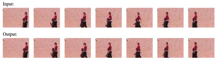
WEXLER ET AL.: SPACE-TIME COMPLETION OF VIDEO 7
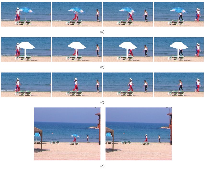
Fig. 7. Removal of a beach umbrella. The video size is 120 340 100, with 422,000 missing pixels. See the video at: http://www.wisdom.weizmann.
ac.il/~vision/VideoCompletion.html. (a) Input sequence. (b) Umbrella removed. (c) Output. (d) Full-size frames (input and output).
for the next level will preserve high spatio-temporal we use the method of [1] so the search time is logarithmic
frequencies and will not be blurred unnecessarily. in K. We typically obtain a speedup of two orders of
magnitude over brute force search. This approach is very
3.3 Algorithm Complexity suitable for our method for three reasons: First, it is much
We now discuss the computational complexity of the faster. Second, we always search for windows of the same
suggested method. Assume we have N ¼ jHj pixels in the size. Third, our robust maximum-likelihood estimation
hole and that there are K windows in the database. The allows us to deal with wrong results that may be returned
algorithm has the following structure.
by this approximate algorithm.
First, a spatio-temporal pyramid is constructed and the
The second stage is the per pixel maximum-likelihood
algorithm iterates a few times in each level (typically, five to
computation. We do this using the Mean-Shift algorithm
10 iterations in each level). Level l contains roughly N=8l hole
[8]. The input is a set of 125 RGB triplets along with their
pixels and K=8l database windows.
Each iteration of the algorithm has two stages: searching weights. A trivial implementation is quadratic in this small
the database and per-pixel Maximum Likelihood. number and so is very fast.
The first stage performs a nearest-neighbor search once The running time depends on the above factors. For
for each window overlapping the space-time hole H. This is small problems, such as image completion, the running
the same computational cost as all the derivatives from Efros time is about a minute. For the “Umbrella” sequence in
and Leung’s work [14]. The search time depends on K and Fig. 7 of size 120 340 100 with 422,000 missing pixels
the nearest-neighbor search method. Since each patch is each iteration in the top level takes roughly one hour on a
searched independently, this step can be parallelized 2.6Ghz Pentium computer. Roughly 95 percent of this time
trivially. While brute-force would take OðK=8l N=8l Þ, is used for the nearest neighbor search. This suggests that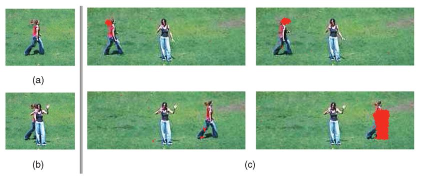
8                                 IEEE TRANSACTIONS ON PATTERN ANALYSIS AND MACHINE INTELLIGENCE,     VOL. 29,   NO. 3,   MARCH 2007

pruning the database (as in [24]) or simplifying the search       contexts, and are therefore only briefly mentioned here.
(as in [2]) would give a significant speedup.                     Other issues are discussed here in more length.
                                                                     Temporal versus spatial aliasing. Typically, there is more
3.4 Relation to Statistical Estimation                            temporal aliasing than spatial aliasing in video sequences of
The above algorithm can be viewed in terms of a statistical       dynamic scenes. This is mainly due to the different nature of
estimation framework. The global visual coherence in (1)          blur functions that precede the sampling process (digitiza-
can be derived as a Likelihood function via a graphical           tion) in the spatial and in the temporal dimensions: The
model, and our iterative optimization process can be seen as      spatial blur induced by the video camera (a Gaussian whose
an approximation of the EM method to find the maximum-            extent is several pixels) is a much better low-pass filter than
likelihood estimate. According to this model, the para-           the temporal blur induced by the exposure time of the camera
meters are the colors of the missing points in the space-time     (a Rectangular blur function whose extent is less than a single
hole and pixels in the boundary around the hole are the           frame-gap in time). This leads to a number of observations:
observed variables. The space-time patches are the hidden
                                                                     1.   Extending the family of Inpainting methods to
variables and are drawn from the data set (patches outside
                                                                          include the temporal dimension may be able to
the hole in our case).
                                                                          handle completion of (narrow) missing video por-
   We show in the Appendix how the likelihood function is
                                                                          tions that undergo slow motions, but there is a high
derived from this model, and that the maximum-likelihood
                                                                          likelihood that it will not be able to handle fast
solution is the best visually coherent completion, as defined             motions or even simple everyday human motions
in (1). We also show that our optimization algorithm fits the             (such as walking, running, etc). This is because
EM method [10] for maximizing the Likelihood function.                    Inpainting relies on edge continuity, which will be
Under some simplifying assumptions, the E step is                         hampered by strong temporal aliasing.
equivalent to the nearest neighbor match of a patch from                      Space-time completion, on the other hand, does
the data set to the current estimated corresponding “hole”                not rely on smoothness of information within patches
patch. The M step is equivalent to the update rule of (3).                and can therefore handle aliased data as well.
   The above procedure also bears some similarity to the             2. Because temporal aliasing is shorter than spatial
Belief Propagation (BP) approach to completion such as in                 aliasing, our multiscale treatment is not identical in
[22]. As BP communicates a PDF (probability density                       space and in time. In particular, after applying the
function), it is practically limited to modeling no more than             video completion algorithm of Section 3, residual
three neighboring connections at once. There, a standard                  spatial (appearance) errors may still appear in fast
grid-based graphical model is used (as is, for example, in                recovered moving objects. To correct those effects,
[16]), in which each pixel is connected to its immediate                  an additional refinement step of space-time comple-
neighbors. Our graphical model has a completely different                 tion is added, but this time, only the spatial scales
structure. Unlike BP, our model does not have links between               vary (using a spatial pyramid), while the temporal
nodes (pixels). Rather, the patch structure induces an implicit           scale is kept at the original temporal resolution. The
connection between nodes. It takes into account not only a                completion process, however, is still space-time. This
few immediate neighbors, but all of them (e.g., 125). This                allows for completion using patches which have a
allows us to deal with more complex visual structures. In                 large spatial extent to correct the spatial information,
addition, we assume that the point values are parameters and              while maintaining a minimal temporal extent so that
not random variables. Instead of modeling the PDF, we use                 temporal coherence is preserved without being
the local structure to estimate its likelihood and derive an              affected too much by the temporal aliasing.
update step using the nearest neighbor in the data set.
                                                                     The local patch size. In our space-time completion process,
   When seen as a variant of belief propagation, one can
                                                                  we typically use 5  5  5 patches. Such a patch size provides
think of this method as propagating only one evidence. In
                                                                  53 ¼ 125 measurements per patch. This usually provides
the context of this work, this is reasonable, as the space of
                                                                  sufficient statistical information to make reliable inferences
all patches is very high dimensional and is sparsely
                                                                  based on this patch. To obtain a similar number of measure-
populated. Typically, the data set occupies “only” a few          ments for reliable inference in the case of 2D image
million samples out of ð3  255Þ125 possible combinations.        completion, we would need to use patches of size 11  11.
The typical distance between the points is very high and, so,     Such patches, however, are not small, and are therefore more
only a few are relevant, so passing a full PDF is not             sensitive to geometric distortions (effects of 3D parallax,
advantageous.                                                     change in scale, and orientation) due to different viewing
                                                                  directions between the camera and the imaged objects. This
4   SPACE-TIME VISUAL TRADE-OFFS                                  restricts the applicability of image-based completion or else
                                                                  requires the use of patches at different sizes and orientations
The spatial and temporal dimensions are very different in         [12], which increases the complexity of the search space
nature, yet are interrelated. This introduces visual trade-offs   combinatorially.
between space and time that are beneficial to our space-time         One may claim that, due to the new added dimension
completion process. On one hand, these relations are              (time), there is a need to select patches with a larger number
exploited to narrow down the search space and to speed            of samples to reflect the increase in data complexity. This,
up the completion process. On the other hand, they often          however, is not the case, due to the large degree of spatio-
entail different treatments of the spatial and temporal           temporal redundancy in video data. The data complexity
dimensions in the completion process. Some of these issues        indeed increases slightly, but this increase is in no way
have been mentioned in previous sections in different             proportional to the increase in the amounts of data.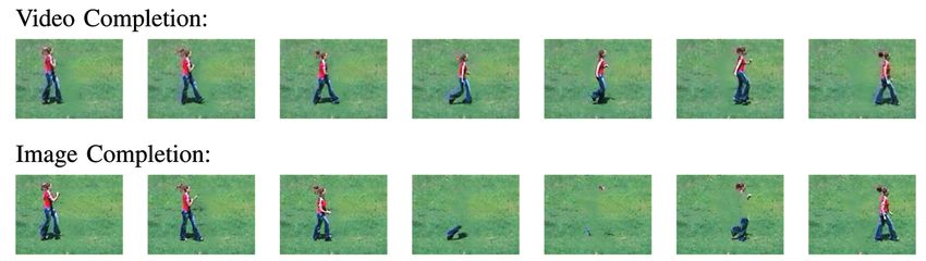
WEXLER ET AL.: SPACE-TIME COMPLETION OF VIDEO                                                                                            9

Fig. 8. Completion of missing frames. The video size is 63  131  42 and has 57,771 missing pixels in seven frames.

Fig. 9. Image completion versus video completion.

   The added temporal dimension therefore provides                       5    UNIFIED APPROACH           TO   COMPLETION
greater flexibility. The locality of the 5  5  5 patches both
                                                                         The approach presented in this paper provides a unified
in space and in time makes them relatively insensitive to
                                                                         framework for various types of image and video comple-
small variations in scaling, orientation, or viewing direction
                                                                         tion/synthesis tasks. With the appropriate choice of the
and, therefore, applicable to a richer set of scenes (richer
                                                                         spatial and temporal extents of the space-time “hole” H and
both in the spatial sense and in the temporal sense).
   Interplay between time and space. Often, the lack of spatial          of the space-time patches Wp , our method reduces to any of
information can be compensated for by the existence of                   the following special cases:
temporal information, and vice versa. To show the impor-                     1.   When the space-time patches Wp of (1) have only a
tance of combining the two cues of information, we compare                        spatial extent (i.e., their temporal extent is set to 1),
the results of spatial completion alone to those of space-time                    then our method becomes the classical spatial image
completion. The top row of Fig. 9 displays the resulting                          completion and synthesis. However, because our
completed frames of Fig. 1 using space-time completion. The                       completion process employs a global objective func-
bottom row of Fig. 9 shows the results obtained by filling in                     tion (1), global consistency is obtained that is other-
the same missing regions, but this time, using only image                         wise lacking when not enforced. A comparison of our
(spatial) completion. In order to provide the 2D image                            method to other image completion/synthesis meth-
completion with the best possible conditions, the image                           ods is shown in Figs. 12, 13, and 14. (We could not
completion process was allowed to choose the spatial image                        check the performance of [12] on these examples. We
patches from any of the frames in the input sequence. It is clear                 have, however, applied our method to the examples
from the comparison that image completion failed to recover                       shown in [12] and obtained comparably good results.)
the dynamic information. Moreover, it failed to complete the                 2.   When the spatial extent of the space-time patches Wp
hopping woman in any reasonable way, regardless of the                            of (1) is set to be the entire image, then our method
temporal coherence.                                                               reduces to temporal completion of missing frames or
   Furthermore, due to the large spatio-temporal redundancy                       synthesis of new frames using existing frames to fill in
in video data, the added temporal component provides                              temporal gaps (similar to the problem posed by [26]).
additional flexibility in the completion process. When the                   3.   If, on the other hand, the spatial extent of the space-
missing space-time region (the “hole”) is spatially large and                     time “hole” H is set to be the entire frame (but the
temporally small, then the temporal information will provide                      patches Wp of (1) remain small), then our method
most of the constraints in the completion process. In such                        still reduces to temporal completion of missing video
cases, image completion will not work, especially if the                          frames (or synthesis of new frames), but this time,
                                                                                  unlike [26], the completed frames may have never
missing information is dynamic. Similarly, if the hole is
                                                                                  appeared in their entirety anywhere in the input
temporally large, but spatially small, then spatial information                   sequence. Such an example is shown in Fig. 8, where
will provide most of the constraints in the completion,                           three frames were dropped from the video sequence
whereas pure temporal completion/synthesis will fail. Our                         of a man walking on the beach. The completed
approach provides a unified treatment of all these cases,                         frames were synthesized from bits of information
without the need to commit to a spatial or a temporal                             gathered from different portions of the remaining
treatment in advance.                                                             video sequence. Waves, body, legs, arms, etc., were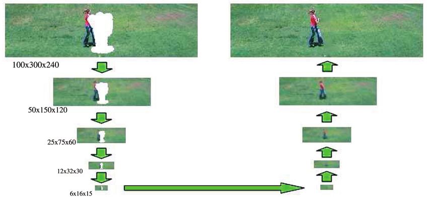
10 IEEE TRANSACTIONS ON PATTERN ANALYSIS AND MACHINE INTELLIGENCE, VOL. 29, NO. 3, MARCH 2007
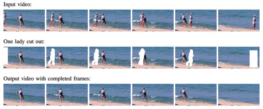
Fig. 10. Removal of a running person. The video size is 80 170 88 with 74,625 missing pixels.
automatically selected from different space-time so, reliance on background subtraction or segmenta-
locations in the sequence so that they all match tion is not likely to succeed here.
coherently (both in space and in time) to each other 2. Restoration of old movies. Old video footage is
as well as to the surrounding frames. often very noisy and visually corrupted. Entire
frames or portions of frames may be missing, and
6 APPLICATIONS severe noise may appear in other video portions.
Space-time video completion is useful for a variety of tasks These kinds of problems can be handled by our
in video postproduction and video restoration. A few method. Such an example is shown in Fig. 11.
example applications are listed below. In all the examples 3. Modify a visual story. Our method can be used to
make people in a movie change their behavior. For
below, we crop the video so to contain only relevant
example, if an actor has absent mindedly picked his
portions. The size of the original videos for most of them is
nose during a film recording, then the video parts
half PAL video resolution (360 288).
containing the obscene behavior can be removed, to
1. Sophisticated video removal. Video sequences often be coherently replaced by information from data
contain undesired objects (static or dynamic), which containing a range of “acceptable” behaviors. This is
were either not noticed or else were unavoidable at demonstrated in Fig. 15, where an unwanted scratch-
the time of recording. When a moving object reveals ing of the ear is removed.
all portions of the background at different time 4. Complete field-of-view of a stabilized video. When a
instances, then it can be easily removed from the video sequence is stabilized, there will be missing
video data, while the background information can be parts in the perimeter of each frame. Since the hole
correctly recovered using simple techniques (e.g., does not have to be bounded, the method can be
[17]). Our approach can handle the more complicated applied here as well. Fig. 16 shows such an application.
case, when portions of the background scene are 5. Creation of video textures. The method is also
never revealed, and these occluded portions may capable of creating large video textures from small
further change dynamically. Such examples are ones. In Fig. 17, a small video sequence (32 frames)
shown in Figs. 1, 7, and 10. Note that, in both Figs. 7 was extended to a larger one, both spatially and
and 10, all the completed information is dynamic and, temporally.
7 SUMMARY AND CONCLUSIONS
We have presented an objective function for the completion
of missing data and an algorithm to optimize it. The
objective treats the data uniformly in all dimensions and the
algorithm was demonstrated on the completion of several
challenging video sequences. In this realm, the objective
proved to be very suitable as it only relies on very small,
local parts of information. It successfully solved problems
with hundreds of thousands of unknowns. The algorithm
Fig. 11. Restoration of a corrupted old Charlie Chaplin movie. The video takes advantage of the sparsity of the database within the
is of size 135 180 96 with 3,522 missing pixels. huge space of all image patches to derive an update step.WEXLER ET AL.: SPACE-TIME COMPLETION OF VIDEO 11
Fig. 12. Image completion example. (a) Original. (b) Our result. (c) Result from [9].
The method provides a principled approach with a clear APPENDIX
objective function that extends those used in other works. In this section, we derive the optimization algorithm from
We have shown here that it can be seen as a variant of EM Section 3 using the statistical estimation framework for the
and we have also shown its relation to BP. interested reader. In this framework, the global visual
There are several possible improvements to this method. coherence of (1) can be derived as a likelihood function via a
First, we did not attempt to prune the database in any way, graphical model and our iterative optimization process can
even though this is clearly the bottleneck with regard to be viewed as a variant of the EM algorithm to find the
running time. Second, we applied the measure to windows maximum-likelihood estimate.
around every pixel, rather than a sparser set. Using a Under this model, the unknown parameters, denoted by
sparser grid (say, every third pixel) will give a significant , are the color values of the missing pixel locations p in the
speedup ð33 Þ. Third, breaking the database into meaningful space-time hole: ¼ fcp jp 2 Hg. The known pixels around
portions can prevent the algorithm from completing one the hole are the observed variables Y ¼ fcp jp 2 S n Hg. The
class of data with another, even if they are similar (e.g., windows fWn gN 1 are defined as small space-time patches
complete a person with background), as was done in [18], overlapping the hole where N is their total number. The set
[24]. Fourth, the proposed method does not attempt to of patches X ¼ fXn gN 1 are the hidden variables correspond-
coalesce identical pixels that come from the same (static) ing to Wn . The space of possible assignments for each Xn
part of the scene. These can be combined to form a joint are the data set patches in D. We assume that each Xn can
constraint rather than being solved almost independently in have any assignment with some probability. For the
each frame as was done here. completion examples here, the data set is composed of all
the patches from the same sequence that are completely
Fig. 13. Texture synthesis example. The original texture (a) was rotated
90 degrees and its central region (marked by white square) was filled
using the original input image. (b) Our result. (c) Best results of (our Fig. 14. The Kanitzsa triangle example is taken from [9] and compared
implementation of) [14] were achieved with 9 9 windows (the only user with the algorithm here. The preference of [9] to complete straight lines
defined parameter). Although the window size is large, the global creates the black corners in (c) which do not appear in (b). (a) Input.
structure is not maintained. (b) Our result. (c) Result from [9].12 IEEE TRANSACTIONS ON PATTERN ANALYSIS AND MACHINE INTELLIGENCE, VOL. 29, NO. 3, MARCH 2007
Fig. 15. Modification of a visual story. The woman in the top row scratches her ear but in the bottom row she does not. The video size is
90 360 190 with 70,305 missing pixels.
Fig. 16. Stabilization example. The top row shows a stabilized video sequence (courtesy of Matsushita [23]) of size 240 352 91 with
466,501 missing pixels. Each frame was transformed to cancel the camera motion and, as a result, parts of each frame are missing (shown here in
red). Traditionally, the video would be cropped to avoid these areas and to keep only the region that is visible throughout. Here, the missing parts
are filled up using our method to create video with the full spatial extent. The results here are comparable with those in [23].
Fig. 17. Video texture synthesis. (a) A small video (sized 128 128 32) is expanded to a larger one, both in space and in time. (b) is the larger
volume of 128 270 60 frames with 1,081,584 missing pixels. Small pieces of (a) were randomly placed in the volume with gaps between them. In
(c), the gaps were filled automatically by the algorithm. Several frames from the initial and resulting videos are shown in (d). (a) Input video texture.
(b) Initial volume. (c) Output video texture. (d) Initial and final resulting texture.
known, i.e., X ¼ fXn jXn S n Hg, but the data set may also Wn denotes a patch overlapping the hole, at least some of
contain patches from another source. these pixel locations are unknowns, i.e., they belong to . Let
This setup can be described as a graphical model which is cp ¼ Wnp denote the color of the pixel p in the appropriate
illustrated in Fig. 18 in one dimension. Each patch Wn is location within the window Wn and let Xnp denote the color
associated with one hidden variable Xn . This, in turn, is at the same location within the data set windows. Note that,
connected to all the pixel locations it covers, p 2 Wn . As each while the color values Xnp corresponding to pixel p may varyWEXLER ET AL.: SPACE-TIME COMPLETION OF VIDEO 13
We will next show that our optimization algorithm fits
the EM algorithm [10] for maximizing the above likelihood
function.
In the E step, at iteration t, the posterior probability
density ^t is computed. Due to conditional independence of
the hidden patches, this posterior can be written as the
following product:
Y
N Y
N
^t ¼ fðXjY; t Þ ¼ fðXn jY; t Þ ¼ n simðXn ;Wn Þ:
n¼1 n¼1
Fig. 18. Our graphical model for the completion problem. Thus, we get a probability value ^t for each possible
assignment of the data set patches. Given the above
for different window locations n, the actual pixel color cp is considerations, these probabilities vanish in all but the best
the same for all overlapping windows Wnp . Using these match assignments in each pixel, thus, the resulting PDF is an
notations, an edge in the graph that connects an unknown indicator function. This common assumption, also known as
pixel p with an overlapping window X n has an edge
“Hard EM,” justifies the choice of one nearest neighbor.
p 2
1
potential of the form ðcp ; Xn Þ ¼ e 22 ðcp Xn Þ . In the M step, the current set of parameters are
The graph in Fig. 18 with the definition of its edge estimated by maximizing the following function:
0 1
potentials is equivalent to the following joint probability X
density of the observed boundary variables and the hidden ^ tþ1 ¼ arg max@ ^t log fðX; Y; ÞA:
patches given the parameters : ðX1 ;...;XN Þ2DN
N Y
Y N Y
Y p
ðcp Xn Þ2
Given the graphical model in Fig. 18, each unknown p
fðY; X; Þ ¼ ðcp ; Xn Þ ¼ e 22 ; depends only on its overlapping patches and the pixels are
n¼1 p2Wn n¼1 p2Wn conditionally independent. Thus, the global maximization
may be separated to local operations on each pixel:
where p denotes here either a missing or observed pixel and
0 1
is a constant normalizing the product to 1. This product is X
exactly the similarity measure defined previously in (2): c^tþ1
p ¼ arg max@ ^ p Þ2 A;
ðcp X n
cp
fn j p2Wn g
Y
N Y
N
^ n are the best patch assignments for the current
fðY; X; Þ ¼ edðXn ;Wn Þ ¼ simðXn ;Wn Þ: where the X
n¼1 n¼1 iteration (denoted also by V in Section 3.1). This is an L2
distance between the point value and the corresponding
To obtain the likelihood function, we need to marginalize color values in all covering patches and it is maximized by
over the hidden variables. Thus, we need to integrate over the mean of these values similar to (3).
all possible assignments for the hidden variables X1 . . . XN : Similar to the classic EM, the likelihood in the “Hard
X EM” presented here is increased in each E and M steps.
L ¼ fðY; Þ ¼ fðY; X; Þ ð5Þ Thus, the algorithm converges to some local maxima. The
ðX1 ;...;XN Þ2DN
use of a multiscale process (see Section 3.2) and other
X Y
N
adjustments (see Section 3.1) leads to a quick convergence
¼ simðXn ;Wn Þ: ð6Þ
n¼1
and to a realistic solution with high likelihood.
ðX1 ;...;XN Þ2DN
The maximum-likelihood solution to the completion
ACKNOWLEDGMENTS
problem under the above model assumptions is the set of
hole pixel values ðÞ that maximize this likelihood function. The authors would like to thank Oren Boiman for pointing
out the graphical model that describes their algorithm and
Note that, since the summation terms are products of all patch
the anonymous reviewers for their helpful remarks. This
similarities, we will assume that this sum is dominated by work was supported in part by the Israeli Science Founda-
the maximal product value (deviation of one of the patches tion (Grant No. 267/02) and by the Moross Laboratory at the
from its best match will cause a significant decrease of the Weizmann Institute of Science.
Q
entire product term): max L maxfXg N n¼1 simðXn ; Wn Þ.
Given the point values, seeking the best patch matches can be
REFERENCES
done independently for each Wn ; hence, we can change the
[1] S. Arya and D.M. Mount, “Approximate Nearest Neighbor
order of the max and product operators: Queries in Fixed Dimensions,” Proc. Fourth Ann. ACM-SIAM
Symp. Discrete Algorithms (SODA ’93), pp. 271-280, 1993.
Y
N
[2] M. Ashikhmin, “Synthesizing Natural Textures,” Proc. 2001 Symp.
max L max simðXn ;Wn Þ; Interactive 3D Graphics, pp. 217-226, 2001.
Xn
n¼1 [3] Z. Bar-Joseph, R. El-Yaniv, D. Lischinski, and M. Werman,
“Texture Mixing and Texture Movie Synthesis Using Statistical
meaning that the maximum-likelihood solution is the same Learning,” IEEE Trans. Visualization and Computer Graphics, vol. 7,
completion that attains best visual coherence according to (1). pp. 120-135, 2001.14 IEEE TRANSACTIONS ON PATTERN ANALYSIS AND MACHINE INTELLIGENCE, VOL. 29, NO. 3, MARCH 2007
[4] M. Bertalmı́o, A.L. Bertozzi, and G. Sapiro, “Navier-Stokes, Fluid Yonatan Wexler received the BSc degree in
Dynamics, and Image and Video Inpainting,” Proc. IEEE Conf. mathematics and computer science from the
Computer Vision and Pattern Recognition, vol. 1, pp. 355-362, Dec. Hebrew University in 1996 and the PhD
2001. degree from the University of Maryland in
[5] M. Bertalmı́o, G. Sapiro, V. Caselles, and C. Ballester, “Image 2001. From 2001 to 2003, he was a member
Inpainting,” ACM Proc. SIGGRAPH ’00, pp. 417-424, 2000. of Oxford’s Visual Geometry Group and, from
[6] T. Chan, S.H. Kang, and J. Shen, “Euler’s Elastica and Curvature 2003 to 2005, he was a researcher at the
Based Inpainting,” J. Applied Math., vol. 63, no. 2, pp. 564-592, Weizmann Institute of Science. He received
2002. the Marr Prize best paper award at ICCV ’03
[7] V. Cheung, B.J. Frey, and N. Jojic, “Video Epitomes,” Proc. IEEE and a best poster award at CVPR ’04. He is a
Conf. Computer Vision and Pattern Recognition, vol. 1, pp. 42-49, member of the IEEE Computer Society.
2005.
[8] D. Comaniciu and P. Meer, “Mean Shift: A Robust Approach Eli Shechtman received the BSc degree magna
toward Feature Space Analysis,” IEEE Trans. Pattern Analysis and cum laude in electrical engineering from Tel-Aviv
Machine Intelligence, vol. 24, no. 5, pp. 603-619, May 2002. University in 1996, and the MSc degree in
[9] A. Criminisi, P. Pérez, and K. Toyama, “Object Removal by mathematics and computer science from the
Exemplar-Based Inpainting,” Proc. IEEE Conf. Computer Vision and Weizmann Institute of Science in 2003. He
Pattern Recognition, vol. 2, pp. 721-728, June 2003. received the Weizmann Institute Dean’s Prize
[10] A.P. Dempster, N.M. Laird, and D.B. Rubin, “Maximum Like- for MSc students, the best paper award at the
lihood from Incomplete Data via the EM Algorithm,” J. Royal European Conference on Computer Vision
Statistical Soc. B, vol. 39, pp. 1-38, 1977. (ECCV ’02), and a best poster award at the
[11] G. Doretto, A. Chiuso, Y. Wu, and S. Soatto, “Dynamic Textures,” IEEE Conference on Computer Vision and
Proc. IEEE Int’l Conf. Computer Vision, vol. 51, no. 2, pp. 91-109, Pattern Recognition (CVPR ’04). He is currently a PhD student at the
2003. Weizmann Institute of Science. His current research focuses on video
[12] I. Drori, D. Cohen-Or, and H. Yeshurun, “Fragment-Based Image analysis and its applications. He is a student member of the IEEE
Completion,” ACM Trans. Graphics, vol. 22, pp. 303-312, 2003. Computer Society.
[13] A. Efros and W.T. Freeman, “Image Quilting for Texture Synthesis
and Transfer,” ACM Proc. SIGGRAPH ’01, pp. 341-346, 2001. Michal Irani received the BSc degree in mathe-
[14] A. Efros and T. Leung, “Texture Synthesis by Non-Parametric matics and computer science in 1985 and the
Sampling,” Int’l J. Computer Vision, vol. 2, pp. 1033-1038, 1999. MSc and PhD degrees in computer science in
[15] A.W. Fitzgibbon, Y. Wexler, and A. Zisserman, “Image-Based 1989 and 1994, respectively, all from the Hebrew
Rendering Using Image-Based Priors,” Int’l J. Computer Vision, University of Jerusalem. From 1993 to 1996, she
vol. 63, no. 2, pp. 141-151, 2005. was a member of the technical staff in the Vision
[16] W.T. Freeman, E.C. Pasztor, and O.T. Carmichael, “Learning Low- Technologies Laboratory at the David Sarnoff
Level Vision,” Int’l J. Computer Vision, vol. 40, no. 1, pp. 25-47, Research Center, Princeton, New Jersey. She is
2000. currently an associate professor in the Depart-
[17] M. Irani and S. Peleg, “Motion Analysis for Image Enhancement: ment of Computer Science and Applied Mathe-
Resolution, Occlusion, and Transparency,” J. Visual Communica- matics at the Weizmann Institute of Science, Israel. Her research
tion and Image Representation, vol. 4, pp. 324-335, 1993. interests are in the areas of computer vision and video information
[18] J. Jia, T.P. Wu, Y.W. Tai, and C.K. Tang, “Video Repairing: analysis. Dr. Irani’s prizes and honors include the David Sarnoff
Inference of Foreground and Background under Severe Occlu- Research Center Technical Achievement Award (1994), the Yigal Allon
sion,” Proc. IEEE Conf. Computer Vision and Pattern Recognition, three-year fellowship for outstanding young scientists (1998), and the
vol. 1, pp. 364-371, 2004. Morris L. Levinson Prize in Mathematics (2003). She also received the
[19] A. Kokaram, “Practical, Unified, Motion and Missing Data best paper awards at ECCV ’00 and ECCV ’02 (European Conference on
Treatment in Degraded Video,” J. Math. Imaging and Vision, Computer Vision), the honorable mention for the Marr Prize at ICCV ’01
vol. 20, nos. 1-2, pp. 163-177, 2004. and ICCV ’05 (IEEE International Conference on Computer Vision), and a
[20] A.C. Kokaram, B. Collis, and S. Robinson, “Automated Rig best poster award at CVPR ’04 (Computer Vision and Pattern
Removal with Bayesian Motion Interpolation,” IEEE Proc.—Vision, Recognition). She served as an associate editor of TPAMI from 1999-
Image, and Signal Processing, vol. 152, no. 4, pp. 407-414, Aug. 2005. 2003. She is a member of the IEEE Computer Society.
[21] V. Kwatra, A. Schödl, I. Essa, G. Turk, and A. Bobick, “Graphcut
Textures: Image and Video Synthesis Using Graph Cuts,” ACM
Trans. Graphics, vol. 22, pp. 277-286, 2003.
[22] A. Levin, A. Zomet, and Y. Weiss, “Learning How to Inpaint from . For more information on this or any other computing topic,
Global Image Statistics,” Proc. IEEE Int’l Conf. Computer Vision, please visit our Digital Library at www.computer.org/publications/dlib.
pp. 305-312, 2003.
[23] Y. Matsushita, E. Ofek, X. Tang, and H.Y. Shum, “Full-Frame
Video Stabilization,” Proc. IEEE Conf. Computer Vision and Pattern
Recognition, vol. 1, pp. 50-57, 2005.
[24] K.A. Patwardhan, G. Sapiro, and M. Bertalmio, “Video Inpainting
of Occluding and Occluded Objects,” Proc. IEEE Int’l Conf. Image
Processing, pp. 69-72, Sept. 2005.
[25] A. Schödl and I. Essa, “Controlled Animation of Video Sprites,”
Proc. First ACM Symp. Computer Animation, (held in conjunction
with ACM SIGGRAPH ’02), pp. 121-127, 2002.
[26] A. Schödl, R. Szeliski, D.H. Salesin, and I. Essa, “Video Textures,”
Proc. ACM SIGGRAPH ’00, pp. 489-498, 2000.
[27] U. Trottenber, C. Oosterlee, and A. Schüller, Multigrid. Academic
Press, Inc., 2000.
[28] L. Wei and M. Levoy, “Fast Texture Synthesis Using Tree-
Structured Vector Quantization,” Proc. ACM SIGGRAPH ’00,
pp. 479-488, 2000.
[29] Y. Wexler, E. Shechtman, and M. Irani, “Space-Time Video
Completion,” Proc. IEEE Conf. Computer Vision and Pattern
Recognition, vol. 1, pp. 120-127, 2004.You can also read