Air Pollution Forecasting and Performance Evaluation Using Advanced Time Series and Deep Learning Approach for Gurgaon
←
→
Page content transcription
If your browser does not render page correctly, please read the page content below
Air Pollution Forecasting and Performance
Evaluation Using Advanced Time Series and
   Deep Learning Approach for Gurgaon

               MSc Research Project
               Msc In Data Analytics

                  Ankit Singh
               Student ID: X18127321

               School of Computing
             National College of Ireland

         Supervisor:   Dr. Pierpaolo Dondio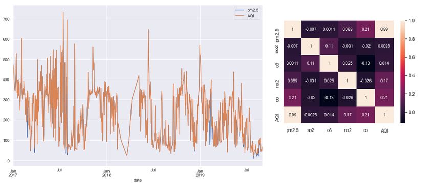
National College of Ireland
                               Project Submission Sheet
                                 School of Computing

 Student Name:                   Ankit Singh
 Student ID:                     X18127321
 Programme:                      Msc In Data Analytics
 Year:                           2019-2020
 Module:                         MSc Research Project
 Supervisor:                     Dr. Pierpaolo Dondio
 Submission Due Date:            12/12/2019
 Project Title:                  Air Pollution Forecasting and Performance Evaluation Using
                                 Advanced Time Series and Deep Learning Approach for Gur-
                                 gaon
 Word Count:                     XXX
 Page Count:                     27

    I hereby certify that the information contained in this (my submission) is information
pertaining to research I conducted for this project. All information other than my own
contribution will be fully referenced and listed in the relevant bibliography section at the
rear of the project.
    ALL internet material must be referenced in the bibliography section. Students are
required to use the Referencing Standard specified in the report template. To use other
author’s written or electronic work is illegal (plagiarism) and may result in disciplinary
action.

 Signature:                 Ankit Singh

 Date:                      11th December 2019

PLEASE READ THE FOLLOWING INSTRUCTIONS AND CHECKLIST:

 Attach a completed copy of this sheet to each project (including multiple copies).
 Attach a Moodle submission receipt of the online project submission, to
 each project (including multiple copies).
 You must ensure that you retain a HARD COPY of the project, both for
 your own reference and in case a project is lost or mislaid. It is not sufficient to keep
 a copy on computer.

    Assignments that are submitted to the Programme Coordinator office must be placed
into the assignment box located outside the office.

 Office Use Only
 Signature:

 Date:
 Penalty Applied (if applicable):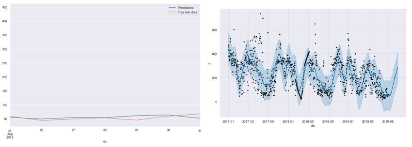
Air Pollution Forecasting and Performance Evaluation
   Using Advanced Time Series and Deep Learning
                Approach for Gurgaon

                                   11th December 2019

                                            Abstract
          Due to its detrimental repercussions, air pollution has been an significant re-
      search area since last few years. Pollution forecasting demands advanced monitor-
      ing stations along with complex algorithms to evaluate time related pollutant data.
      Accurate air quality forecasting is critical for systematic pollution control as well as
      public health and wellness. An Indian city Gurugram has been ranked as the highest
      polluted city in the world since last two years by AirVisual. Advanced forecasting
      models can be implemented on considerable pollutant datasets to get valuable future
      forecasts that aid government health organisations to adopt precautionary measures.
      This study involved the utilisation of novel forecasting model Prophet to predict the
      future pollution precisely. The obtained results were compared with several statist-
      ical, time series and deep learning models such as AR, ARMA, ARIMA, SARIMA,
      Exponential Smoothing, TBATS and LSTM in terms of forecasting error and other
      factors. Model evaluation has been carried out on 8-hourly pollution data using
      multiple evaluation metrics such as RMSE, MSE, MAE and MAPE. The results
      obtained have been evaluated and visualised. Research findings signify Prophet to be
      the most efficient forecasting model with the lowest combined evaluation errors in-
      cluding RMSE, MAE, MSE and MAPE proving capable of handling outliers, trend
      and seasonality in data. Prophet also gave good performance on a separate Delhi
      data. This approach can assist in improving the current forecasting quality thereby
      benefitting the country and its people.
      Index Terms : Air Pollution, Forecasting, AQI, Time Series, Deep Learn-
      ing, PROPHET

1     Introduction
1.1    Background
Air pollution has been one of the major concerns for developing countries such as India
since the last few years. Air pollution has caused the most number of deaths in the
near past and the count keeps increasing every year. Numbers show that more than
660 million Indians breathe polluted air every day. Breathing polluted air can cause
fatal cardiovascular and lung related diseases such as lung cancer, asthma and ischaemic

                                                 1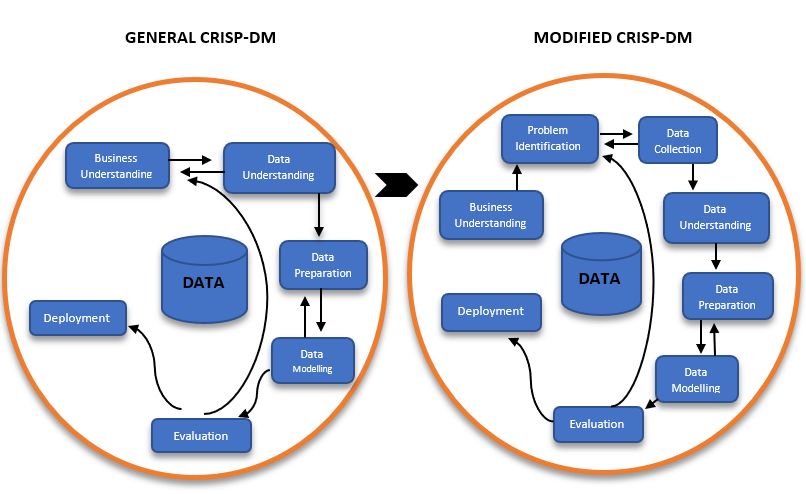
heart disease. Air Quality Index is the measure adopted by the Indian government
to quantify air pollution. Different air pollutants and meteorological factors like SO2,
NO2, PM2.5, PM10, Humidity, Wind Direction and Speed are the considered for the
calculation of the AQI. AQI is a measure which is accepted all over the world by most
countries Kumar and Goyal (2011a). AirVisual which is a popular pollution monitoring
site has ranked a north Indian city Gurgaon as the most polluted city in the world since
2018. This is the reason for selecting Gurgaon as the test location. Currently, three
major approaches are being implemented for forecasting specifically Chemical Transport,
Statistical Methods and Machine Learning Deters et al. (2017),Xi et al. (2015) . Statistical
models have been implemented in the past to forecast pollution . The major issue that
has been experienced with statistical modelling is producing negative correlation among
meteorological variables Deters et al. (2017),Xi et al. (2015). Chemical transport models
are much complex in nature and difficult to improve. Machine learning has been found
out to be the best choice for most researches as it provides the flexibility to consider
several parameters for modelling Deters et al. (2017),Xi et al. (2015) . However, most
researches done on Indian air pollution doesn’t involve advance forecasting models and
method to make accurate prediction. Important time related data aspects such as missing
values, trends, outliers and seasonality should be handled in order to make better precise
predictions. In this research advanced Prophet model has been utilised which is capable
of handling all the features of time related data. The model would be compared with
several other models such as ARMA, ARIMA, SARIMA, Exponential Smoothing and
LSTM. Since a single evaluation metric would not be trustworthy, model evaluation
would be accomplished with several metrics RMSE, MSE, MAE and MAPE.

1.2    Motivation
Following the World Health Organisation air pollution standards would add 4.7 years of
life to every living individual in India. To maintain the pollution and take prevention
measures, accurate future forecasting is required. As per Deters et al. (2017), 3 million
people die every year in the world due to outdoor air pollution. Gases like NO2, O3 and
CO harm the nervous system and cause inflammation Gu et al. (2018). Sharma et al.
(2018) mentions that the concentration of SO2 and O3 are going to increase in the future
years. As per Li et al. (2017), India is going to beat china for SO2 concentration. In
order to control the diseases and deaths, advanced air quality monitoring and forecasting
mechanisms are required. Presently, the forecasting systems only provide real time data
which is not effective for handling future pollution crisis. Many diseases and deaths can
be avoided with the assistance of an accurate forecasting model. Leaving the government
and environmental organisations aside, people living the country would be aided directly
with a future air quality level indicator model.

1.3    Project Requirement Specification
The ascending issue of air quality degradation affecting thousands of lives across India
(Gurgaon) in the absence of an effective forecasting models has been discussed in the
research question stated below:

RQ1: “Can several advanced state-of-the-art time series and deep learning models along
with a novel PROPHET model be implemented and compared on forecasting Air Quality

                                             2
of Gurgaon, India using parameters such as CO2, SO2 and PM2.5?”

RQ2: “Can novel Prophet model beat the current state-of-the-art models in terms of
forecasting errors ?”

1.4    Achieved Objectives
Following objectives have been achieved from this research project : 1.

                              Table 1: Objectives Achieved
 Objectives           Description
 Objective 1          An investigation and assessment of Indian air pollution data of Gurgaon
 Objective 2          Data gathering, preprocessing involving the calculation of Indian Air
                      Quality Index.
 Objective 3          Implementation of a novel Prophet model on the pollutant data of Gur-
                      gaon
 Objective 4          Comparison of multiple forecasting models which include AR, ARMA,
                      ARIMA, Seasonal ARIMA, TBATS, Exponential Smoothing and
                      LSTM
 Objective 5          Evaluating the applied models using several evaluation metrics RMSE,
                      MSE, MAE and MAPE
 Objective 6          Getting the most accurate model with respect to the forecasting errors
 Objective 7          Representing the results in the form of visualisations and generating
                      insights from it

1.5    Project Contributions
The research project has lead to the following contributions :

  1. The primary contribution associated with the project would be to deliver a complete
     and accurate pollution forecasting model thereby contributing to the environment
     and people health.

  2. Comparing modern state-of-the-art model with models being used in the past in
     terms of forecasting accuracy to find the best performing model.

1.6    Project Outline
In the next stages of the paper, section II provides a detailed criticism of relevant re-
searches and literature published in the past. This section is the backbone for this
research project as every steps taken has been compared and referred from the literature
reviewed. Third section explains the research methodology and scientific design adopted.
Section IV discusses the several methods and models implemented on Gurgaon air pollu-
tion data. Section V explains the evaluation of the applied models in terms of multiple
metrics. The last section gives the references to the literature cited.

                                            3
2 A Critical Review of Researches and Literature
Relevant to Air Pollution and Forecasting (2001-
2019)
2.1 Introduction
Air pollution has been regarded as a critical and dangerous issue all over the world espe-
cially in growing industrial countries such as India. According to Deters et al. (2017) ,
different machine learning and statistical methods like time series modelling, deep learn-
ing and linear modelling has been applied in forecasting air quality. However, current
researches like Neto et al. (2017) have implemented specific machine learning methods
like deep learning and time series more effective and popular. Literature review would
lay a strong foundation for this research project as all the implementation and evaluation
methods have been based upon the strengths and limitations observed in the reviewed
literature. The complete critical analysis of the literature has been separated into men-
tioned subsections to provide more clarity to the reader :
1. Critical evaluation of papers on Air Pollution and Forecasting (Section 2.2)
2. Critical evaluation of literature on the basis of research variable used (Section 2.3)
3. Critical evaluation of research papers on different time series models implemented
(Section 2.4)
4. Critical evaluation of papers on various deep learning methods used in air quality
forecasting (Section 2.5)
5. Critical review of literature based on various evaluation criteria adopted (Section
2.6)
Major papers, journals and articles referred in this research has been cited from either
IEEE Xplore, NCI Library or Google Scholar.
2.2 Critical Evaluation of Papers on Air Pollution and Fore-
casting
In a research conducted by P. Singh et al. (2013), a high correlation was discovered
between daily mortality rate and air pollution data. Guo et al. (2018) mentioned about
PM2.5 being one of the deadliest air pollutant as it can penetrate the lungs. Similarly,
Ul-Saufie et al. (2011) also mentioned about the deadly diseases like asthma and chest
pain caused to workers due to particulate matter like PM2.5 and PM10. Kumar and
Goyal (2011a) got average performance by applying general statistical methods like mul-
tiple linear regression to predict future pollution. Another research conducted by Cogliani
(2001) implemented linear regression models for prediction. The major issue that came
out from the research was correlation among the different features.
Most researches had used basic statistical models which were not accurate due to cor-
relation and disability to model several other time series factors such as trend, seasonality
and outliers. This gap has been handled in this project by using advanced time series
and deep learning models capable of better forecasting the air quality.
42.3 Critical Evaluation of Literature on the Basis of Research
Variable Used
Research variable and predictor variables play an important role in any machine learning
project. Mishra (2016) Due to its deadly repercussion, air quality degradation is an sens-
itive issue nowadays. For accurate forecasting, careful measures should be undertaken for
choosing the correct research variable and its predictors. Niska et al. (2004) forecasted
NO2 using predictors like Ozone, Sulphur di oxide, PM210 and Carbon Monoxide for
Helsinky city. Kurt et al. (2008) implemented neural networks utilised multiple pollut-
ants like SO2, CO, PM10, NO and O3 to predict SO2, PM1 and CO levels for Istanbul
data. Another forecasting project carried out by Athanasiadis et al. (2003) picked Ozone
as the forecasting variable. According to Silva et al. (2013), PM2.5 and Ozone accounted
for over 2 million deaths around the world. Apart from air gases and particulate matter,
certain meteorological factors such as wind speed, wind direction and air temperature
are also correlated with the air quality and assist in predicting the same. Most discussed
researches did not include meteorological for forecasting the air pollutants. Guttikunda
and Gurjar (2011) found out correlation among the meteorological factors and the overall
pollution. In a similar study conducted by Chaloulakou et al. (2003) found out a direct
relationship between temperature, wind speed and air pollution. An analysis was done
by Guttikunda and Gurjar (2011) to find the effect of meteorological factors on pollu-
tion. It was discovered that pollution tend to increase by 40-80 percent in the winters
than summers. This directly shows the effect of temperature on pollution. The above
discussed issue of including meteorological factors in the research was handled by Kumar
and Goyal (2011b). They considered an aggregation of both air pollutants and met-
eorological factors like pressure, temperature and rainfall for forecasting. The research
included general statistical models like linear regression and ARIMA. The drawback of
the research being absence of any advanced forecasting model capable of handling non-
linear data.
Identified Gap: Most researches have used PM2.5 or NO2 as their research variable.
However, predicting a single pollutant would not accurately represent the overall air
quality. In order to resolve this drawback in selecting the research variable, a collect-
ive air quality indicator has been used all around the world represented by Air Quality
Index. Kumar and Goyal (2011b) and P. Singh et al. (2013) handled this drawback by
forecasting AQI for Delhi and Lucknow using general statistical models. AQI is a term
used by the government to calculate and represent the overall air pollution Sharma et al.
(2018). As per the Central Pollution Control Board of India, AQI is calculated taking all
available pollutant and meteorological data into consideration which must include either
PM2.5 or PM10. Future AQI can be forecasted and categorised according to the national
standards for common people to understand and take preventive measures in advance. In
this research, the gap has been filled by calculating the AQI from the available pollutant
data and forecasting it in the future. Due to insufficient meteorological data, weather
and geographical factors have not been included in this research. However, this limitation
can be a part of the future scope or improvement for this project.
52.4 Critical Evaluation of Research Papers Involving Different
Time Series Models
Past researches show general statistical models to be inefficient in forecasting non-linear
pollution data due to several drawbacks including correlation, trend, seasonality and out-
liers. Zhao et al. (2018) mentioned machine learning models to be better in comparison
with statistical methods. In their research, Kumar and Goyal (2011a) used general models
such as linear regression and were unable to get above average performance in AQI fore-
casting. Moreover those models were not able to provide important information such as
outliers, overall trend and daily or weekly seasonality. As discussed in the earlier section,
Cogliani (2001) also faced the problem of correlation among variables while forecasting
the pollution of multiple cities. Kumar and K. Jain (2010) by implemented ARIMA
model to forecast air pollution of Delhi. Auto correlation and partial auto-correlation
plots were utilised to find the input parameters for the model. Since the above plots
are difficult to interpret, auto-arima has been implemented in this project as it finds
the best parameters for ARIMA automatically. However, one limitation for the project
was that ARIMA model is incapable of handing seasonality in data, which according to
Guttikunda and Gurjar (2011) is present in Indian air data. In order to remove this
limitation of ARIMA, Rahman et al. (2016) implemented seasonal ARIMA model which
was able to provide better results by capturing seasonality as well. The model performed
better on urban areas. As this model was able to perform better than ARIMA, it has
been implemented in this project along with ARIMA for comparison. Neto et al. (2017)
found general statistical linear models to be inefficient against time series pollution data
containing outliers, trend or seasonality. Another issue with Indian pollution data is
the presence of multiple seasonality which most models including Garch were unable to
recognise while forecasting. Guttikunda and Gurjar (2011) found the relation between
both as it was analysed that pollution in winter season was much higher than summer
seasons. So the applied model should have the capability of handling multiple seasonality.
M. De Livera et al. (2010) used an advanced forecasting model called TBATS along with
Exponential Smoothing. It is a combination of several models and is capable of handling
more than one type of seasonality and data with high correlation. TBATS is a collection
of several methods namely Trigonometric, Box Cox, ARMA errors, Trend and Seasonal-
ity. This model has performed well in most researches but hasn’t been implemented in
most Indian researches. Due to its capability of handling multiple seasonality TBATS
and Holt Exponential Smoothing has been implemented in this project.
Research Gap: The major issue with most forecasting models is the incapability of hand-
ling peak or outliers, random lags, trend, seasonality with accurate forecasting. None
of the current applied forecasting models are efficient in handling data with peaks or
outliers. Most general models are cabling of handling one or two of the above time series
data features but there is a need of a model capable of handling peaks and other time
series characteristics as well simultaneously.
In order to fill this gap, a novel advance forecasting model named Prophet has been
implemented in this project on the air pollution data of Gurgaon. This model has been
developed recently by Facebook and is capable of handling large random lags in data
as well as holidays or peaks. Apart from this Prophet is capable of handling multiple
seasonality and trend in the data as well. Kolehmainen et al. (2001) mentioned in the
research about the issue of fitting spiked data to the general models. Yenidoğan et al.
6(2018) compared the forecasting accuracy of Prophet and ARIMA on bitcoin data. In the
research it was found out that the R square value of Prophet to be 94 percent when com-
pared to 68 percent of ARIMA. The model was designed by Facebook for stock market
data containing multiple trends, seasonality and outliers. Since Indian air quality data
has similar features with respect to stock market data, Prophet has been implemented as
a novel model in this research. As no paper was found involving Prophet on Indian air
pollution data, it provides the novelty in this research.
2.5 Critical evaluation of papers on various deep learning meth-
ods used in air quality forecasting
Along with time series models, deep learning have also performed well in terms of fore-
casting air pollution. Deep learning has been used in most recent researches involving air
pollution forecasting. Kolehmainen et al. (2001) got impressive results using neural net-
works to forecast Nitrogen dioxide concentration for Stockholm. Ul-Saufie et al. (2011)
and Caselli et al. (2009) compared feed forward neural network with multiple regression
on air data and found neural network to be the better performer in terms of root mean
squared error. However, all of the above researches had a drawback of not being able
to model peaks, falls and huge lags in the data. In a study by Guo et al. (2018) Feed
forward neural network outperformed boosting and random forest algorithms with re-
spect to multiple evaluation methods. In spite of high forecasting performance of deep
learning models, the major limitation is having short term making them unable to re-
member long past values while forecasting the future. Tsai et al. (2018) and Tao et al.
(2019) implemented a deep learning model called Long Short Term Memory capable of
considering the long past values while predicting the future. In both researches LSTM
outperformed multiple models including Support Vector Machine, boosting and decision
tree methods. In the research by Tsai et al. (2018), LSTM outperformed Artificial Neural
Network as well. Due to the high performance and long term memory of LSTM, it has
been implemented in this research.
Identified Gaps: Moreover, no Indian air quality forecasting paper has been found which
compared time series models with deep learning methods. By implementing a collection
of multiple time series, statistical and deep learning prediction models this would be a
novel research on Indian air pollution data. The prediction error of novel Prophet model
would be compared against all applied model in order to find the most accurate and
efficient air pollution forecasting model.
2.6 Critical Review of Literature Based on Various Evaluation
Criteria Adopted
Evaluation is a critical step in any research project implementation. Each and every
model or method implemented should be evaluated using one or several metrics for trust-
worthy result. Without proper evaluation, a project can be declared as untrustworthy or
unauthentic. Caselli et al. (2009) used Root Mean Square Error as the evaluation criteria
for forecasting PM2.5. Multiple Linear Regression and Artificial Neural Network were
applied and evaluated. Hyndman and Koehler (2006) has mentioned the limitation of
RMSE to be good with scaled data only. Similarly, Kolehmainen et al. (2001) applied
neural networks to forecast pollution on the data of Stockholm, Sweden. RMSE was the
7evaluation measure adopted in the research. Since RMSE represents the mean errors,
it is sensitive to outliers. Niska et al. (2004) used neural networks along with parallel
genetic algorithm to forecast the Nitrogen Di-oxide concentrations of Helsinky. Regu-
larised Mean Squared Error was used for evaluation. GA performed better than neural
network getting low RMSE value. However, by using single evaluation criteria it cannot
be assured that the test results are fully trustworthy.
One major drawback of the above papers was the usage of a single evaluation metrics.
This drawback was overcome by Tao et al. (2019) in their research involving deep learn-
ing models to forecast Beijing PM2.5 concentrations. Good performance was achieved
with applied deep learning models. Several evaluation criteria namely Mean Absolute
Error, Root Mean Square Error and Symmetric Mean Absolute Percent Error were used
to evaluate the performance of the models. In another research involving deep learning
techniques by Tsai et al. (2018), Root Mean Squared Error and Mean Absolute Error
were applied to evaluate the performance of the models. The intuition behind using the
metrics was that RMSE is able to evaluate the level of change of the data and accuracy
and MAE gives the actual error values which are in the same unit as the data. In a similar
way Ying Siew et al. (2008) applied models such as ARFIMA and ARIMA to forecast
the air pollution of Malaysia. Model evaluation was done using a number of evaluation
metrics including RMSE, MAE and MAPE were used in order to get validated results.
Identified Gaps: Most researches lack the implementation of several evaluation metrics
which provides variety and trustworthy results. Different evaluation metrics has different
advantages and drawbacks as suggested by Hyndman and Koehler (2006) in a research.
Hyndman and Koehler (2006) compared multiple scale dependent and independent evalu-
ation methods and found MAE to be better for scaled data and Mean Absolute Percentage
Error good for non-scaled data. Wang et al. (2015) got impressive results using MAPE
as their evaluation metrics. In order to get trustworthy results several evaluation metrics
like RMSE, MAPE, MAE and MSE has been implemented in this project.
3 Methodology Adopted
3.1 Introduction
A modified version of CRISP-DM has been adopted as the methodology in this project
Rocha and de Sousa Junior (2010) . Several other processes such as Knowledge Discovery
in Databases and SEMMA (Sample, Explore, Modify, Model, and Assess) are also being
used in the industry. In the paper by Nadali et al. (2011), it is mentioned that most
processes including KDD and SEMMA lack business understanding which is an important
aspect for the research project. Due to this important feature, CRISP-DM is being
utilised in half of the companies and their data analytic projects Nadali et al. (2011).
Being an academic research project, it should also solve a real world problem along with
adding some business value. In order to meet the project requirements, two additional
modifications have been made to the general CRISP-DM architecture. The modified
version of the general methodology has been discussed below.
3.2 Modified Project Methodology
The modified CRISP-DM methodology is presented below (1) :
8Figure 1: Modified CRISP-DM Methodology Proposed
3.2.1 Business Understanding and Problem Identification
The research project deals with the rising problem of air pollution in India. Solving
this problem would directly aid the government and people living in the country. This
problem provides the motivation behind the research project. An accurate model capable
of accurately modelling Indian pollution data could be utilised by the environmental
government organisations for better air quality forecasts.
3.2.2 Data Collection and Understanding
Data gathering and exploration is an important aspect of any data related projects. Data
collected should be authentic and real. Most Indian air pollution researches have gathered
their data from the website of Central Pollution Control Board of India. CPCB is an
authentic Indian government organisation responsible for recording air quality data for
most Indian cities using monitoring stations nationwide. Most pollution researches done
on Indian cities have taken the data from CPCB Sharma et al. (2018).
The data for this project has been gathered from the Central Pollution Control Board
website 1 . Being the most polluted city in the world, Gurgaon has been chosen as the test
location. Dataset ranges from 1/01/2017 until 31/08/2019 containing 8 hourly concen-
trations of air pollutants namely Sulphur Di-oxide, Ozone, Carbon mono-oxide, Nitrogen
di-oxide and Particulate Matter 2.5. As per the official CPCB document, Indian air pol-
lutant concentration varies every 8 hours at minimum. For this reason 8 hourly data has
been used in this project. Apart from this, another reason behind selecting 8 hourly data
was high missing data points. Choosing 24 hourly data would have resulted in missing
dates thereby making imputation difficult. As per CPCB, a minimum of three pollut-
ant data is necessary for the calculation of AQI, one of which should be either PM10 or
PM2.5. Keeping this in mind, data has been gathered. Since Gurgaon is a new city and
the air quality monitoring stations have been recently installed, enough meteorological
data was not found to be included in the research. However, by plotting and analysing
1
https://app.cpcbccr.com/ccr/#/caaqm-dashboard/caaqm-landing/data
9the gathered pollution data it was found out that PM2.5 accounted for ninety nine per-
cent of the AQI values as the sub-indices of it being the highest among all pollutants.
It went in accordance with the CPCP official pollution document as particulate matter
being the most responsible pollutant affecting the AQI.
Exploratory data analysis: Exploratory data analysis has been carried out using Excel,
R and Python (Spyder). The dataset downloaded had several rows of redundant data
which needed to be removed along with a CPCB logo. As the file was in excel format,
’read excel’ function was used in R to read the file and the first 15 redundant rows were
omitted using skip function. EDA functions such as shape, info and describe were used in
python for understanding and exploring the dataset further. Matplotlib library was used
for visually exploring the separate pollutant concentrations. After plotting the calculated
AQI, no visible trend or seasonality was found. Statistical tests for confirming the same
has been discussed in the coming sections.
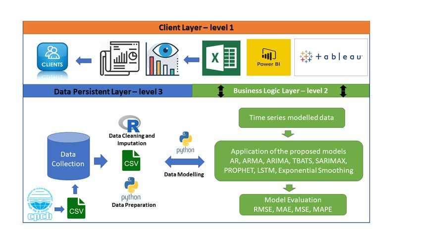
Correlation Analysis: Correlation analysis in the figure2 below shows that PM2.5 is the
major pollutant contributing about 99 percent to the overall AQI. This goes according
to CPCB as particulate matter being the most responsible pollutant for air pollution in
India. It can be seen that the plot of AQI and PM2.5 almost overlap as well. As per the
AQI generation formula, PM2.5 concentrations are the maximum everyday (Figure2)
Figure 2: Correlation Analysis
3.2.3 Data Preparation
Preprocessing is the process of making data model ready. It involves several stages such
as missing value removal, handling white spaces, making calculations and splitting of data
into train and test. Preprocessing was the most time consuming part of this project as
the data needed cleaning and transformation to get it model ready. The dataset gathered
had 5 columns namely SO2, O3, CO2, NO2 and PM2.5. As daily data was required
by the novel Prophet model, the datetime column was separated using ‘tidyr::separate’
function in R. All the columns were converted into numeric and all 0’s were replaced with
null so that they could be imputed more conveniently. ‘Since we were focusing on daily
data, ‘to date’ column was removed as it was not required.
10Figure 3: Missing Values
Handling Missing Data Points : Missing values in a time series dataset can reduce
the forecasting performance immensely. If the missing lag is long, it can affect the overall
forecast. ‘Is.na’ function was applied to the dataset to get the number of missing values.
Out of 21233 datapoints, 2103 were missing. Upon exploration, it was noticed that the
data points were not missing at random. Moreover, there were long continuous lags in
the data. As the air quality monitoring stations go under maintenance, few consecutive
days of data can get missed in a month.
Zakaria and Noor (2018) did a comparative study on several types of imputation methods
being used on time series data. Methods such as multiple imputation, mean of top and
bottom and nearest neighbour were implemented and compared. Mean top bottom was
found out to be the best imputation method. However, as pollution data varies after
every 8 hours, mean top bottom would not be a good choice as it would replace the
missing value by the average of its previous and next value. Moshenberg et al. (2015)
used spectral imputation method to fill the missing values. It was found out that the
method was not efficient when the missing data size was large or the data was not missing
at random. Other imputation method like forward and backword fill or pairwise deletion
would not be effective as the data can have seasonality, trend or outliers.
In order to resolve all the drawbacks of the above mentioned methods, a method in-
volving seasonal adjustment along with linear interpolation has been adopted in this
project. As mentioned in ‘towardsdatascience2 ’, this method can handle time series data
with both trend and seasonality. Other methods such as mean, mode and median are
not good at handling time stamped data. This method is useful if there are long missing
gaps in the data. ‘na.seadec’ function was applied to the dataset to fill the missing data-
points. All missing values were filled by first adjusting the seasonality if any and then by
interpolating. The dataset was then saved as a csv and imported to Python for further
processing and transformation.
Transformation: After reading the csv in Python, the column containing the date and
time was transformed into datetime format for Python and models to understand. This
was done using the pandas library function ‘pd.to datetime’. As the format of the date
2
https://towardsdatascience.com/how-to-handle-missing-data-8646b18db0d4
11was not default in the csv used, it was specified in the function. As all the columns apart
from datetime had integers with decimal values, those columns were converted to float
and the 8 hourly data was aggregated to daily data by using a user-defined-function.
The reason behind aggregation was that the novel Prophet model takes daily data as its
parameter. In order to convert the dataset into time series, the date column was set as
an index. Since AQI has been chosen as the research variable, its calculation has been
explained in the following section.
AIR QUALITY INDEX: AQI is the measure accepted all around the world to represent
pollution as it is calculated from the combined pollutant data. Different countries have
different formulas to calculate AQI from pollutants. Multiple researches like Wang et al.
(2017), Kumar and Goyal (2011b), P. Singh et al. (2013) and Cogliani (2001) have used
AQI as their research variable. Kumar and Goyal (2011a) in their research adopted US
aqi formula to calculate the air quality index. As mentioned by Feng et al. (2015), AQI
is used to represent the complete pollutants data into a single column so that it can be
forecasted easily and accurately. To calculate the AQI for this project, an AQI calculator
has been used. It has been created by the Central Pollution Control Board of India and is
freely available to calculate accurate AQI values from a given pollutant data. The calcu-
lator was available at https://app.cpcbccr.com/ccr_docs/AQI%20-Calculator.xls.
Being in an excel format, the formula for calculating the sub-indices of different pollut-
ants were gathered and implemented in the csv itself and five new sub-indices columns
were generated. From those sub-indices the maximum values were taken as the AQI for
a particular day. The formula for calculating the sub-indices can be stated as follows:
Figure 4: AQI Formula
Kumar and Goyal (2011a) used US-AQI to calculate the AQI for their data. In the
official document published by CPCB at http://www.indiaenvironmentportal.org.
in/files/file/Air%20Quality%20Index.pdf, most AQI’s has been compared with the
IND-AQI. Fenstock AQI is not applicable for daily data forecasting. Similarly, to calculate
Ontario API has only two pollutants SO2 and COH included in its formula. It does not
include the value of particulate matter, which is one of the most important pollutant
responsible for air pollution in India. As per CPCB, the major issue with most AQI’s is
that their formula suffer from ambiguity and eclipsing as most formula add the sub-indices
of separate pollutants to get the AQI. For example if two sub-indices are 70 and 80, their
addition would result in 150 which is higher than the pollution standards. However, the
actual values for sub-indices are below the pollution range. This produces ambiguity and
eclipsing in data. IND-AQI resolves this drawback by taking the maximum value of all
available sub-indices to calculate AQI. After the AQI has been calculated in excel, it
has been read into python and the pollutant data columns have been removed to make
the data ready for modelling. The final dataset has an AQI column along with a date
column index and is ready for further analysis followed my modelling. First two research
objectives have been achieved after the completion of data preprocessing.
123.2.4 Data Modeling
Tests for Stationarity: Before fitting models on the data, several tests were implemen-
ted as well. These tests confirmed the validity of the dataset to be used for time series
forecasting. The most important fact that separates time series data project from any
other is Stationarity. Stationary time series implies that there is no specific trend or
seasonality in the data. General classification or regression projects do not have time
related features such as trend or seasonality. Most pollution researches done on air pol-
lution found their data to be non-stationary as pollution tend to change from season to
season or month to month. Models such as AR, ARMA and ARIMA are not efficient in
handling non-stationary data. So in order to use these models, stationarity tests were
done. Autocorrelation and Partial auto correlation plots were implemented. Statistical
variance and mean summary tests showed that the dataset had different variance and
mean for different intervals, implying the data to be non-stationary. Gaussian distribu-
tion has also been checked using histogram plot in Python, which showed the series to be
skewed. However, general plots can be deceiving to the human eye. Augmented Dickey
Fuller Test and Kwiatkowski.Phillips.Schmidt.Shin test were implemented to check the
stationarity of the dataset. Both ADF and KPSS are the two most popular statist-
ical tests being used for time series. The output of both the tests showed the data to
be stationary. Seasonal decomposition also shows no presence of clear seasonality in data.
As the data came out to be stationary, all the models have been directly applied as
no differencing was needed. Auto Regression with different lags (AR1, AR2, AR19),
ARMA, ARIMA, Simple Exponential Smoothing, SARIMAX, LSTM, TBATS, Rolling
ARIMA has been implemented along with the novel PROPHET model for comparison,
although only top performing models have been mentioned in the project report. The
research objective involving implementation of all the models have been achieved after
this stage. Detailed explanation of the models implemented has been discussed in the
later implementation section 5.
3.2.5 Evaluation
Model evaluation has been carried out using several evaluation metrics to get trust-
worthy results. As per the literature reviewed Tsai et al. (2018), Ying Siew et al. (2008)
state-of-the art popular evaluation metrics like MAE, RMSE, MSE and MAPE has been
implemented in the project. Upon evaluation, PROPHET came out to be the most accur-
ate forecasting model in terms of every evaluation metrics applied. All models have been
evaluation on the basis of both weekly and monthly forecasts. Apart from the evaluation
metrics, the PROPHET model has also been tested on a new dataset of Delhi
Mean Squared Error: MSE is obtained by taking the average of squared forecasted errors
in any prediction. Due to the squared errors, large forecasting differences are converted
to even bigger errors by squaring them. So outliers increase the MSE values abruptly.
Since the MSE of PROPHET came out to be the least among all models, it shows that
the novel Prophet is capable of handling outliers effectively.
13Figure 5: MSE (yi and yi is the test and prediction values)
Mean Absolute Error: Mean Absolute error can be described as the average of all
forecast errors, where all forecasted values are positive. MAE in not sensitive to outliers
as it takes the direct absolute forecast difference between the test and predictions. This
provides MAE an advantage over mean squared error as it is very sensitive to outliers.
Since there are a number of peak values in the data, MAE has been chosen as the primary
evaluation metric.
Figure 6: MAE (yt and yt is the test and prediction values)
Root Mean Squared Error: RMSE is basically the square root of the obtained Mean
Squared Error. The general advantage of RMSE over MSE is that RMSE has the same
units as the data making it easier to interpret. RMSE is one of the most popular eval-
uation metrics with respect to time series projects. Most reviewed researches such as
Kolehmainen et al. (2001) and Ying Siew et al. (2008) has selected RMSE to be their
evaluation metrics.
Figure 7: RMSE (N means number of time data points and Pi, Oi are the predictions
and Observations)
Mean Absolute Percentage Error: Most evaluation metrics such as MSE and RMSE
are scale dependent. So they are not so reliable when the data has different scales. Since
the project is on univariate time series, there is only one column to be forecasted. Scaling
is required when there are multiple variables of different scales. The main advantage of
MAPE is that it is scale independent. Several popular air pollution researches such as
Wang et al. (2015) included MAPE as their evaluation metrics. Inclusion of MAPE has
provided variety to this research.
Figure 8: MAPE (xi and xi represent the predicted and observed values and n denotes
the number of predictions)
14By implementing all the above mentioned evaluation metrics, research objective has
been achieved.
3.2.6 Deployment
In an industrial point of view, deployment refers to the release of a model or software
in the market for use. As the research project is for academic purpose, visualisations
of the performance results obtained along with the project report constitutes as the
deployment. Moreover, as it is evident from the results that the novel Prophet model has
outperformed other compared state-of-the-art mode, this project or model can be used
by the environmental agencies for better forecasting.
4 Project Design Architecture
4.1 Introduction
A three tier architecture has been utilised for the research project. Most software Industry
projects use three tier architecture. The reason behind using a three tier architecture is
that the project covers all the three level of architecture including Data, business logic
and client layer.
Figure 9: Data flow Diagram
4.1.1 Data Layer
The data layer goes in accordance with the data collection layer of crisp-dm methodology.
For this project, the data has been downloaded as an csv from the official CPCB website
https://app.cpcbccr.com/ccr/#/caaqm-dashboard/caaqm-landing/data. All data
related calculations and preprocessing has been done in this layer.
154.1.2 Business Logic Layer
Business logic layer deals with the application and evaluation of all the models and
algorithm. This layer is the intermediary layer between the client and data. All the
models and evaluation metrics mentioned in the later section has been implemented as a
part of this layer.
4.1.3 Client Layer
This layer is the outmost layer of the architecture dealing with the client end of the
project. After the completion of the modelling and evaluation phase, the results were
noted and visualised by using several tools like Tableau, PowerBI and matplotlib(python).
An academic report has been created containing all the details about the implementation
and insights for the end user to understand.
5 Implementation, Evaluation Along with Analysis
of Results Obtained from Pollution Forecasting Mod-
els
5.1 Introduction
Implementation and Evaluation are two major parts in any data analytic project. For
this project, Python(Spyder) has been used for model implementation and evaluation.
Analysis and visualisation of results has been done using Python and Tableau. Most
packages were already available in Python, the rest were installed using ‘pip install’
function. Most time series models were available in ‘statsmodel’ package. All plotting
functions like ‘pacf’, ‘acf’ and ‘lag plot’ were either called from ‘pandas’ or ‘statsmodel’.
Implementation helped in achieving the research objective.
Lag Plot Correlation Check: Since the project had a univariate time series AQI column.
Unlike general classification or regression projects, correlation in time series refers to
plotting a time series at time x(t) on x-axis with the same time series at time x(t+1) on
y-axis. The lag plot shows a positive correlation among the time series at different time
intervals. According to the obtained lag plot, the time series is good for forecasting the
future.
Figure 10: Lag Plot
16Auto-correlation and Partial-autocorrelation: PACF and ACF plots are used to find
the complete and partial autocorrelation values of a time series with its past lagged values.
ACF finds the correlation with lagged values and PACF finds the autocorrelation with
the residuals. Kumar and De Ridder (2010) AR and MA order can be found out from the
ACF and PACF plots. It can be noticed that almost all the lags lie inside the confidence
interval which is by default 95 percent. As almost all lags lie inside the CI. However,
these plots can be misleading and difficult to interpret.
Figure 11: ACF and ACF
Augmented Dickey Fuller and Kwiatkowski Phillips Schmidt Shin Test3 : As plots can
be misleading and can give the wrong idea about whether the series is stationary or not,
ADF and KPSS tests were used to confirm the nature of time series data. ADF checks
the null hypothesis that whether the time series can be represented by a unit root or not
and KPSS checks whether or not the time series is trend stationary. ADF and KPSS
tests are opposite in nature. ‘adfuller’ and ‘kpss’ functions were used .
Figure 12: Stationarity Tests
As the p-value of KPSS is more than 0.05 and the p-value of ADF is less than 0.05,
both tests prove the time series to be stationary.
Decomposition: Time series can have multiple components such as trend, residuals and
seasonality. Due to seasonality, the pollution can be different in winters then sum-
mers. In order to check the above features, decomposition was done on the data. ‘sea-
sonal decompose’ function was used from the ‘statsmodel’ library. It was noticed that no
clear trend or seasonality was seen in the plot.
3
https://www.analyticsvidhya.com/blog/2018/09/non-stationary-time-series-python/
17Figure 13: Seasonal Decomposition
5.2 Model Implementation and Evaluation
This section deals with the implementation and evaluation of applied models individually.
5.2.1 Implementation and Evaluation of Exponential Smoothing Forecasting
Model
Exponential smoothing has been implemented using the ‘ExponentialSmoothing’ func-
tion from the library ‘statsmodels.tsa.holtwinters’. Parameters like trend and seasonality
were set to multiplicative rather than additive as there was no visible growing trend in
the plot. As no clear seasonality was seen in the seasonal decomposition, several values
for the parameter ‘seasonal periods’ were tried and the best results were obtained with 4
seasonal periods. The reason can be that Indian weather has 4 different seasons in a year.
Triple exponential smoothing was used as it can also model hidden trend or seasonality
M. De Livera et al. (2010).
Evaluation: RMSE, MSE, MAE, MAPE and the total execution time was calculated
using function ‘time.time’ imported from the library ‘time’. The results show the model
to be giving average forecasts. Exponential Smoothing gave better long term forecast in
comparison with short term weekly forecast.
Forecasts RMSE MSE MAE MAPE Execution Time(sec)
7 Days 42.1 1777 40 80.4 0.34
30 Days 38.7 1501.1 28.4 38 0.429
5.2.2 Implementation and Evaluation of Auto-Regressive(AR) Forecasting
Model
AR model uses an auto-regressive term to model time series. It basically uses an term to
represent the current state series x(t) with its passed vales. It calculates a term p, which
represents the number of past value required to generate the current values Kumar and
K. Jain (2010). AR model was tested for three different lags that is 1,2 and 19 where
19 was the best performer. A parameter (ic=’t-stat’) was used to get the best lag value
18which came out to be 19. It can be seen in the graph below, forecasting got better by
increasing the lags.
Figure 14: AR Model
Evaluation: Since, AR19 gave the best performance compared to AR1 and AR2, the
results of AR19 has been discussed. Similar to exponential smoothing, AR also performed
better for long term predictions. The overall performance of AR was not satisfactory but
the execution time was impressive. Model was not able to capture changes in data.
Forecasts RMSE MSE MAE MAPE Execution Time(sec)
7 Days 67 4501 66 128 0.013
30 Days 37 1405 30 62 0.018
5.2.3 Implementation and Evaluation of ARMA Forecasting Model
Autoregressive moving average model or ARMA is a collection of two separate processes
namely autoregression and moving average. Similar to AR it used an auto-regression
component ‘p’ and combines it with an additional moving average component ‘q’ Kumar
and K. Jain (2010). The comparison between the forecast and true data can be seen in
the below image. (figure 15
Figure 15: ARMA Model
19Evaluation: The performance of ARMA model increased for long term forecasts
though the execution time was more or less constant. The model was not able to capture
the changes, peaks and falls in the data.
Forecasts RMSE MSE MAE MAPE Execution Time(sec)
7 Days 74 5497 73 141 0.382
30 Days 40.8 1665 31.8 66 0.388
5.2.4 Implementation and Evaluation of ARIMA Forecasting Model
Since, the performance of ARMA was not satisfactory, ARIMA was implemented. AR-
IMA is one of the most utilised time series model. Most researches has implemented
ARIMA to be the baseline for their research Kumar and K. Jain (2010). ARIMA is the
combination of autoregressive(p) and moving average(q) separated by a differencing term
‘d’. ARIMA is represented as ARIMA(p,d,q) and the values of these parameters were
obtained using a function called ‘auto arima’ which was taken from the library ‘pmdar-
ima’. Since ACF and PACF plots can be mis-leading or difficult to interpret, auto-arima
checked different parameters by passing them into arima to get the best values. The
best values were found to be p=2, d=1, q=2. ‘.predict’ function was used to make the
predictions.
Evaluation:ARIMA performed better than ARMA for short term forecasting but the
performance of ARIMA was not good compared to ARMA for 30 days forecast.
Forecasts RMSE MSE MAE MAPE Execution Time(sec)
7 Days 74 5497 73 141 0.382
30 Days 40.8 1665 31.8 66 0.388
5.2.5 Implementation and Evaluation of SARIMA Forecasting Model
SARIMA is the extension of ARIMA by adding an additional component of seasonality
to it. Since, there was no visible seasonality in the seasonal decomposition, SARIMA was
implemented in comparison to ARIMA. SARIMA was introduced by Box and Jenkins.
Multiple researches like Gocheva-Ilieva et al. (2013) showed that SARIMA was able to
model the seasonality present in the data thereby giving better forecast. SARIMA can
be represented by the following:
SARIMA(p,d,q)(P,D,Q,M)
Where p,d,q are the ARIMA terms and P,D,Q,M refers to the seasonal auto-regressive
order, seasonal difference, seasonal moving average and number of time steps in a single
season
Evaluation: Auto-arima was used to get the best order values for test. Auto-arima
gave SARIMAX(1,1,1) as the best model. SARIMAX performed better than ARIMA
showing that some seasonality may be present in the data. The performance improved
for long term forecasting and the execution time was low as well. Overall, SARIMA
forecasted the value with good accuracy and less error.
Forecasts RMSE MSE MAE MAPE Execution Time(sec)
7 Days 37 1398 36 71 0.23
30 Days 26 711 21 36 0.188
205.2.6 Implementation and Evaluation of LSTM Forecasting Model
LSTM stands for long short term memory. It is a type of recurrent neural network cap-
able of remembering long past values to make the future predictions. This capability of
LSTM makes it stand out from other deep learning models for pollution forecasting Tsai
et al. (2018). The capacity of LSTM in handling volatility in the data was discussed
by Kong et al. (2019) in their research. This model has outperformed popular models
like K- nearest neighbour and back propagation neural network by forecasting accurate
short term power load for New South Wale data. Since LSTM requires scaled data,
‘MinMaxScaler’ function was imported from the ‘sklearn.preprocessing’ library to scale
the data. As deep learning models require the data to be in a particular format, Instead
of directly fitting the model on train data, a function named ‘timeseriesgenerator’ was
imported from the ‘keras’ library and fitted on the scaled train data by specifying the
number of input as 30 and features as 1 with batch size of 30.
Evaluation: Thirty epochs were made on model fit and the loss function graph was
also generated. The evaluation of short and long term lstm forecasting has been dis-
cussed below:
Forecasts RMSE MSE MAE MAPE Execution Time(sec)
7 Days 101 10240 99 190 59.9
30 Days 116 13667 106 212 47.2
5.2.7 Implementation and Evaluation of TBATS Forecasting Model
TBATS is a collection of several features like Trigonometry, Box-Cox to handle hetero-
geneity, ARMA error, Trend and Seasonality. M. De Livera et al. (2010) mentioned the
advantages of TBATS in comparison with other time series model. As TBATS is good in
handling complex seasonality and the seasonal decomposition on the data did not showed
clear seasonality, it was implemented in the project. ‘TBATS’ function was used and the
‘seasonal periods’ parameter was set to yearly seasonality. Both short and long term
forecasting was done using ‘forecast’ function. It was seen that though TBATS was not
able to model the peaks in data but it was close to the mean.
Figure 16: TBATS Model
Evaluation: Model was evaluated with the four evaluation metrics along with exe-
cution time. It is seen that TBATS model gave good forecasting results, especially for
long term forecast. The execution time was found to be higher.
21Forecasts RMSE MSE MAE MAPE Execution Time(sec)
7 Days 56 3174 55 108 109.5
30 Days 32 1062 25 38 79.5
5.2.8 Implementation and Evaluation of PROPHET Forecasting Model
Implementing PROPHET was the novelty for this research as no papers were found in-
volving its application to predict Indian air pollution. It is a newly developed forecasting
model launched by Facebook engineers, and is capable of handling most time series fea-
tures such as holidays, outliers, trend and seasonality4 . ‘Prophet’ function was imported
from ‘fbprophet’ library. The columns were converted to the format ‘ds’, ’y’ as the model
needs the dataset in this format. The predictions were stored in a future dataframe hav-
ing the predicted dates as an index. ‘make future dataframe’ function was used to create
the dataframe and ‘predict’ was used forecast values.
Figure 17: PROPHET Model
The major insight which was found upon implementation was that prophet was able
to model the peaks and falls in the data better all the compared models. Thus it could
help in solving the drawback of fitting spikes which occurred in most research like Koleh-
mainen et al. (2001) . In the second image containing the forecast, blue line refers to the
actual forecasted future values, black dot represent the data points available and light
blue region refers to the confidence interval or the degree of variance.
Evaluation: Prophet gave the lowest errors on all evaluation metrics for short term
air pollution forecast. The execution time recorded was quite high in comparison to
other models.
Forecasts RMSE MSE MAE MAPE Execution Time(sec)
7 Days 9 85 7 13 3.27
30 Days 35 1295 26 36 6.55
Delhi Data 34 1169 29 7 2.8
Evaluation of Prophet on Delhi Data: As Prophet outperformed all applied models,
In order to further test the forecasting accuracy of Prophet, it was applied to a new New
Delhi test data. It was found out that Prophet gave accurate predictions with low values
of MAE, MAPE and RMSE considering the AQI values were higher in Delhi data.
4
https://research.fb.com/prophet-forecasting-at-scale/
22Figure 18: PROPHET Components
‘plot components’ is an inbuilt feature of prophet to plot different aspects such as
trend and weekly seasonality. Prophet’s inbuilt cross validation was also performed. The
pollution was found to be higher on weekends and in winter months which is not surprising
since people tend to travel during weekends and temperature is lower in winters. In the
inbuild cross validation metric plot, it was seen that the mape value of Prophet remains
more or less constant in all time intervals that is 0-60 days forecast.
6 Analysis of Results Obtained
After successful evaluation of separate models, a combined evaluation matrix and fore-
casts were created to compare and contrast all the models applied.
Figure 19: Plotted Predictions
23You can also read