Crime is in the Air: The Contemporaneous Relationship between Air Pollution and Crime - IZA DP No. 11492 APRIL 2018
←
→
Page content transcription
If your browser does not render page correctly, please read the page content below
DISCUSSION PAPER SERIES

IZA DP No. 11492

Crime is in the Air:
The Contemporaneous Relationship
between Air Pollution and Crime

Malvina Bondy
Sefi Roth
Lutz Sager

APRIL 2018
DISCUSSION PAPER SERIES

IZA DP No. 11492

Crime is in the Air:
The Contemporaneous Relationship
between Air Pollution and Crime
Malvina Bondy
London School of Economics
Sefi Roth
London School of Economics and IZA
Lutz Sager
London School of Economics

APRIL 2018

Any opinions expressed in this paper are those of the author(s) and not those of IZA. Research published in this series may
include views on policy, but IZA takes no institutional policy positions. The IZA research network is committed to the IZA
Guiding Principles of Research Integrity.
The IZA Institute of Labor Economics is an independent economic research institute that conducts research in labor economics
and offers evidence-based policy advice on labor market issues. Supported by the Deutsche Post Foundation, IZA runs the
world’s largest network of economists, whose research aims to provide answers to the global labor market challenges of our
time. Our key objective is to build bridges between academic research, policymakers and society.
IZA Discussion Papers often represent preliminary work and are circulated to encourage discussion. Citation of such a paper
should account for its provisional character. A revised version may be available directly from the author.

                                           IZA – Institute of Labor Economics
Schaumburg-Lippe-Straße 5–9                      Phone: +49-228-3894-0
53113 Bonn, Germany                             Email: publications@iza.org                                    www.iza.org
IZA DP No. 11492                                                                                                                 APRIL 2018

            ABSTRACT
            Crime is in the Air:
            The Contemporaneous Relationship
            between Air Pollution and Crime*
            Many empirical studies have examined various determinants of crime. However, the link
            between crime and air pollution has been surprisingly overlooked despite several potential
            pathways. In this paper, we study whether exposure to ambient air pollution affects crime
            by using daily administrative data for the years 2004-05 in London. For identification, we
            mainly rely on the panel structure of the data to estimate models with ward fixed effects.
            We complement our main analysis with an instrumental variable approach where we use
            wind direction as an exogenous shock to local air pollution concentrations. We find that
            elevated levels of air pollution have a positive and statistically significant impact on overall
            crime and that the effect is stronger for types of crime which tend to be less severe. We
            formally explore the underlying mechanism for our finding and conclude that the effect
            of air pollution on crime is likely mediated by higher discounting of future punishment.
            Importantly, we also find that these effects are present at levels which are well below
            current regulatory standards and that the effect of air pollution on crime appears to
            be unevenly distributed across the income distribution. Overall, our results suggest that
            reducing air pollution in urban areas may be a cost effective measure to reduce crime.

            JEL Classification:              H23, K42, Q53
            Keywords:                        air pollution, crime, economic incentives

            Corresponding author:
            Sefi Roth
            The London School of Economics and Political Science
            Houghton Street
            London WC2A 2AE
            United Kingdom
            E-mail: s.j.roth@lse.ac.uk

            * We would like to thank Mirko Draca for sharing his data on crime in London and Gabriel Ahlfeldt and Felipe
            Carozzi for their helpful comments. Sager gratefully acknowledges financial support by the Grantham Foundation for
            the Protection of the Environment and the UK’s Economic and Social Research Council (ESRC).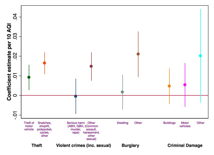
I.       Introduction

         Over the past few decades, crime has been a major policy issue in both national and

local politics due to its significant social and economic cost. According to an official

government report, the total cost of crime in England and Wales is approximately £60 billion

per year1. This figure, which is far from comprehensive, suggests that effective crime reduction

measures have the potential to provide substantial savings. Indeed, a large body of literature

studying the determinants of crime has offered several potential measures to tackle crime such

as increased police presence and better education (Draca et al., 2011; Machin et al., 2011)2.

However, the link between improved air quality and crime reduction has been surprisingly

overlooked in the empirical literature despite several potential pathways.

         In this paper, we study whether short-term exposure to elevated levels of ambient air

pollution affects crime in London. We believe that London provides an almost ideal setting for

this type of study for two main reasons. First, the high quality of the daily administrative crime

data, in conjunction with the extensive network of air pollution monitoring stations, allows us

to overcome the many identification problems, such as measurement error and the presence of

unobserved correlated factors. Second, London is similar to many major cities around the world

in terms of its characteristics. According to the 2017 Economist Safe Cities Index and recent

figures from the World Bank, both pollution and safety levels in London are almost identical

to other major cities such as Chicago and New York3. Therefore, our results should be of

1
  This figure is taken from the Home Office Research Study 217 which was published in 2000. In 2005, the Home
Office revised the estimates for the total cost of crime against individual and households to about £36.2 billion
per year but this figure does not include crimes against business and the public sector.
2
  Policymakers also tend to focus on these measures. For example, the mayor of London recently claimed that
real-terms cuts in various public services such as community education and the police had “reversed decades of
progress in tackling the root causes of violent offending” (The Independent, 2018).
3
  The 2017 Economist Safe Cities Index, which ranks 60 major cities around the globe, placed London in the
20th spot for overall safety (between Chicago (19) and New York (21)). The pollution data is for PM10.

                                                       1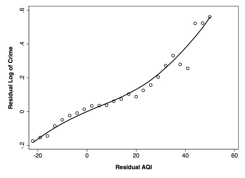
particular interest to policymakers not just in London, but also to those in many other large

cities around the world.

         We estimate the effect of air pollution on crime using a unique data set, which combines

readings of ambient air pollution concentrations with rich administrative records on over 1.8

million criminal offences recorded in London during the years 2004-2005. To account for

potential confounders we take the following measures. First, we rely on the panel structure of

the data to estimate models with ward fixed effects. Second, we complement our main analysis

with an instrumental variable approach, where we use wind direction as an exogenous shock

to local air pollution concentrations. Finally, we perform a range of robustness and placebo

tests, which provide additional support to the causal interpretation of our analysis.

         The results suggest that exposure to elevated levels of air pollution is associated with

increased crime rates. In our preferred fixed effects specification we find that an additional 10

Air Quality Index (AQI) points increase the crime rate by 0.9% and experiencing an AQI of

above 35 leads to 2.8% more crimes. The latter result, which is equivalent to 0.07 of a standard

deviation, is very large and similar to the estimated effect of a 9% decrease in police activity

(Draca et al., 2011)4. Our instrumental variable approach, which uses wind direction as an

instrument that can flexibly influence pollution at different locations, yields statistically similar

results. More specifically, we find that additional 10-instrumented AQI points increase crime

rate by 1.7%. Finally, we explore whether ambient air pollution has heterogeneous effects on

crime types and across the income distribution. We find that the effect is stronger for types of

crime which tend to be less severe and that the effect appears to be unevenly distributed across

resident income groups.

4
 Draca et al. (2011) focus on the effect of increased police presence following the July 2006 terror attacks in
London.

                                                        2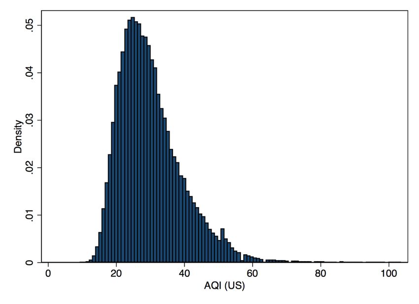
To explain the underlying mechanism for our findings, we complement our empirical

results with a formal economic framework rooted in the rational choice theory of crime

(Becker, 1968). In the context of this framework, we expect short-term fluctuations in air

pollution to influence criminal activity through any of the following three channels – (i)

altering perceived payoffs, (ii) altering risk perceptions, or (iii) altering risk preferences. Based

on our empirical results we conclude that the effect of air pollution on crime is likely mediated

by higher discounting of future punishment.

        Overall, this study provides several important contributions to the literature on crime,

as well as carrying important implications for public policy more broadly. First, our results

suggest that improving air quality in urban areas may provide a cost effective way to reduce

crime. Second, the link between pollution and crime suggests that the optimal deployment of

law enforcement resources (e.g. local police personnel) should incorporate information from

pollution forecasts. Third, our results are present at levels which are well below current US

Environmental Protection Agency (EPA) and UK Department for Environment, Food & Rural

Affairs (DEFRA) standards which suggests that it may be economically beneficial to lower

existing guidelines. Finally, this study also contributes to the evolving body of research

studying the link between ambient pollution and the impact on other aspects of human life such

as productivity, cognitive performance and sports performance (Graff-Zivin and Neidell, 2012;

Ebenstein et al., 2016; Lichter et al., 2017). More specifically, given the link between air

pollution and crime, our results therefore suggest that examining the effects of air pollution on

health impacts alone may lead to a substantial underestimation of its societal costs.

                                                 3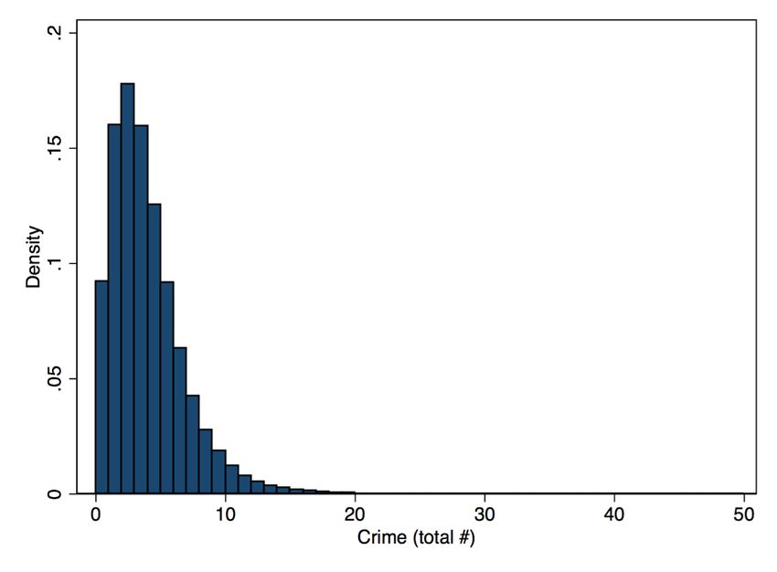
II.      Background and Conceptual Framework

         a. The Adverse Effects of Air Pollution on Human Life

         The adverse health effects of ambient air pollution are well-established in the

epidemiology and economic literature. Early epidemiological studies documented a strong

association between extreme pollution events, such as the London Great Smog, and mortality

(Logan, 1953). Later studies, which evaluate the link between pollution and health with lower

and more common air pollution levels, found that ambient pollution affects life expectancy and

hospitalisation (Dockery et al., 1993; Pope et al. 1995). The economic literature, which better

accounts for potential confounders, has also documented a strong link between air pollution

and various health outcomes such as infant mortality and emergency room visits (Chay and

Greenstone, 2003; Schlenker and Walker, 2015). More recently, a new wave of studies has

examined the impact of pollution on other aspects of human life. For example, Graff Zivin and

Neidell (2012) presented robust evidence for a causal link between ozone and productivity of

agricultural workers in California; Ebenstein et al. (2016) found that elevated levels of PM2.5

reduce student test scores among Israeli students; Sager (2016) documented a robust causal

relationship between pollution and road safety in the UK; and Lichter et al. (2017) showed that

variation in pollution affects professional soccer players in Germany.

         Despite this growing body of literature on the adverse effects of air pollution on many

aspects of human life, the evidence on the link between pollution and crime is extremely

scarce5. To the best of our knowledge there are only three papers in the economic literature

which examine somewhat related links. The first two papers (Reyes, 2007; 2015) examine the

link between childhood lead exposure and crime rates later in life in the United States. The

         5
            There are a few studies that examine the effect of other environmental factors, such as temperature, on
crime. For example, a number of studies find a significant association between temperature and violent as well as
property crimes (e.g. Ranson, 2014; Cohen and Gonzalez, 2018). A recent review of the literature on climate and
conflict is provided by Burke et al. (2015).

                                                        4
first paper uses state-year panel data to examine within state variation in lead exposure and
crime. The results suggest that lead exposure during childhood is associated with violent crimes
but not with property crimes. The second paper also finds a link between early childhood lead
exposure and criminal behaviour, using data on two cohorts of children from the NLSY.
Finally, a working paper by Herrnstadt et al. (2016) examines the contemperenous link
between pollution and crime in Los Angeles and Chicago. Similar to several other studies on
air pollution (Anderson, 2015; Deryugina et al., 2016), they also use daily wind direction as an
instrument for ambient air pollution. More specifically, they compare relative criminal activity
on opposite sides of major interstates in Chicago, on days when the wind blows orthogonally
to the direction of the interstate. In LA, they compare crimes in communities on the foothills
of the San Gabriel Mountains with those in other parts, on days with and without winds blowing
from the ocean towards this region6. Overall, they find that violent crime in Chicago increase
by 2.2% per day on the downwind side of the interstate with no effect on property crime. In
Los Angeles, they find a 19.4% increase in assaults for a 10ppb increase in ozone exposure.
Their paper is the closest one to our study but there are several important differences between
the two. Most notably, whilst they remain agnostic regarding the underlying mechanisms, we
investigate the influence of pollution on crime within a rational choice framework. By
combining our theoretical framework with our empirical evidence, we are able to provide
strong evidence that pollution raises crime rates through a change in the cost-benefit trade-off.
Furthermore, we analysed a wide range of crime types and find that pollution affects not only
violent, interpersonal crime (which is the focus of their paper), but also a range of other
crimes including those that are more economically motivated. Finally, we also provide some
6
The logic here is that the San Gabriel Mountains trap the pollution in communities on its foothills during these
days.
5evidence regarding the distributional aspects, where we analyse the relationship between air
pollution and crime across resident income groups.
b. Conceptual Framework: Pollution and Crime
To better understand the mechanism for the potential link between pollution and crime
we embed our analysis in the canonical rational choice model of crime proposed by Becker
(1968) and Ehrlich (1973), which characterises the supply of criminal activity as driven by
individual decision making under risk7. Following Becker (1968), a potential offender j
chooses to commit an offence if her expected utility from the crime outweighs the utility of a
certain outside option, so if:
!" $" %"& − ()"& + 1 − !" $" %"& > $" %"-&
Given a fixed outside option %"-& 8, any potential offender j is more likely to commit an offence
if: (i) the payoff from crime %"& increases relative to the cost of future punishment )"& which is
discounted at the rate (, (ii) the probability of being punished !" is lowered, or (iii) the
potential offender’s preferences $" . become more risk accepting9 10.
As outlined above, exposure to air pollution has been linked to changes in behaviour,
productivity and well-being. In the context of the rational choice framework, we may expect
short-term fluctuations in air pollution to influence criminal activity through any of the
7
We choose rational choice as our guiding framework in understanding the relationship between acute exposure
to air pollution and criminal activity. Rational choice is only one of many frameworks to understand criminal
behaviour. Other prominent theories focus for example on persistent personality traits (e.g. Nagin & Paternoster,
1993) or social structure (Saw & McKay, 1942; Bursik, 1988) – with both of these examples less applicable for
the short-term (daily) fluctuations in crime that are the subject of our analysis.
8
A large share of the economics of crime literature focuses on longer term determinants of crime, so that %"-&
might for example correspond to earnings from legitimate work. In our framework, which focuses on short-term
decisions, %"-& may reflect factors shaping the utility of refraining from committing an offence on that given day.
9
There is indeed robust evidence that the expected gain as well as the likelihood and magnitude of punishment
do influence the supply of offences in the expected direction. Most recently, Draca et al. (2018) find substantial
responses of property crimes to commodity prices in the United Kingdom for the years 2002-2012.
10
Alternatively, we can use a more common additive time separable formulation as follow:
U1 W13,5 + p1 U1 W17 − S15 + 1 − p1 U1 W17 > U1 W13,95 + U1 W17
6following three channels – (i) altering perceived payoffs (%"& and ()"& ), (ii) altering risk
perceptions (!" ), or (iii) altering risk preferences ($" . ). In principle, a potential influence of
air pollution may then either increase or decrease criminal activity. For example, if elevated
levels of air pollution lead to increased risk aversion, we would expect to see a decrease in
criminal activity on high polluted days. Conversely, if air pollution reduces expected cost of
future punishment, via lower discounting (() for example, we would expect to observe increase
in crime on days with pollution. We will discuss evidence for each of these possible channels
with our results below.
III. Data
Our final data set combines several files which contain administrative information on
crime rates, ambient air pollution, weather and various demographics. For crime information,
we use data from the London Metropolitan Police Service which contains ward level detailed
daily police reports of all recorded crimes in the Greater London area for the years 2004-200511.
Importantly, the data allows us to know not just the number of crimes per ward per day, but
also the type of crime. Furthermore, the file also provides data on police deployment, tube
journeys and unemployment levels which were originally obtained and defined as follow. Data
on police deployment was taken from the police service’s human resource management system
and contains the total weekly number of hours worked by officers for each of the 32 boroughs
in London. The weekly data on total number of tube journeys was taken from Transport for
London (TFL) and information on borough’s unemployment levels were taken from the UK
Quarterly Labour Force Survey (LFS)12.
11
This data file is taken from Draca et al. (2011). The file does not include data on the City of London, which is
one of the 33 local authority districts of Greater London.
12
In our analysis we divided the weekly total number of tube journeys in each borough by the number of tube
stations in the same borough.
7For information on pollution and weather, we use daily data from the Department for
Environment Food and Rural Affairs (DEFRA, 2017) and the Met office (2012). These files
provide information on daily means of five pollutants, temperature, relative humidity, rainfall
and wind direction and speed from 96 monitoring stations in the London area (see figure 1). In
our analysis we use the AQI, which is calculated according to the US EPA formula, as our
main pollution measure. More specifically, we define the overall daily AQI as the highest AQI
among the individual pollutants, which is in line with the EPA reporting guidelines.
We assign pollution and weather to wards by linking it with the three monitoring
stations closest to the ward centroid. We then use the mean value of those three measurements
weighted by the inverse squared distance between station and ward. We also attempted
alternative approaches of assignment and the results are nearly identical. Finally, we add
population data from London’s Ward Atlas (2017) and data on house prices by ward from the
Land Registry (2017) to test whether the effect of pollution on crime varies across the resident
income groups13.
Table 1 presents summary statistics for our key variables of interest. Our sample
includes 455,520 observations of daily crime counts (over 1.8 million criminal offences in
total) across 624 wards in London14. The average daily AQI and the number of crimes per
100,000 people during our sample period were 30.06 and 34.06 respectively. Figure 2 plots the
distributions of AQI and total number of crimes in our sample. In columns (2)-(3) of Table 1
we stratify the sample by the median house price. As expected, we don’t find meaningful
differences in temperature, relative humidity and rainfall. However, the table indicates that
13
The alternative approaches are (1) using only the reading from the station closest to each ward (2) using the
closest valid reading from the three closest stations.
14
The day of the July 2005 attack is dropped from the sample (reducing it to 730 days) leaving a sample of
730*624=455,520 observations.
8both, pollution levels and the number of crimes, are higher in wards where house prices are
above the median.
IV. Empirical Strategy
There are several identification challenges for inferring a causal link between pollution
and crime. The prime concern is the possible presence of unobserved correlated factors. For
example, if pollution is higher in poorer areas, a naïve OLS estimate might overstate the effect
of pollution on crime, as crime may be higher in those areas for other correlated reasons (e.g.
lower quality of education). We overcome this and other related econometric challenges by
using two separate identification strategies as follow.
a. Panel Fixed Effects Model:
In our first empirical approach, we crucially rely on the panel structure of the data to
estimate models with ward fixed effects. More formally, we estimate models of the following
form:
;?@ABCD ) = bFGHCD + I JBA!CD , KLCD + M%@varying conditions potentially related to pollution and crime16. µt and gi are time and ward fixed
effects respectively. Finally, eit is an idiosyncratic error term.
Through the inclusion of ward fixed effects our identification relies on the comparison
of crime levels between days with higher and days with lower pollution levels within the same
ward. This approach removes any potential confounding from time-invariant structural
differences between wards, which as mentioned above, is a prime concern.
Weather controls are included because of well documented evidence which show that
weather conditions can influence both pollution levels (Zannetti, 2013) and criminal activity
(Burke et al., 2015; Cohen & Gonzalez, 2018). We also include further control variables
intended to account for time-varying local conditions that may influence criminal activity. Tube
activity acts as a proxy for general levels of activity and crowdedness, which may again
influence both pollution and crime. Unemployment rates and the level of police deployment
serve as additional controls for potentially confounding factors. It is conceivable that more
police officers being deployed influences both pollution and crime. Similarly, we may
hypothesise that short-term fluctuations in unemployment are associated with both levels of
pollution and crime17.
A final concern may be periodic co-movement between pollution and crime unrelated
to the causal effect hypothesised above. For example, we may expect busy weekdays to differ
from quiet Sundays both in pollution levels and criminal activity. To account for such
systematic time-varying factors, we include in RD a collection of time fixed effects. These
include dummies for the Day of the Week to counter the potential short-run seasonality
16
We rely here on the following control variables from the data compiled by Draca et al. (2011): borough-level
unemployment rate, the number of tube journeys (separately measured for weekdays and the weekend), and the
(natural logarithm of) total hours of police deployment. These characteristics vary by week.
17
As these variables may also be seen as outcomes of the treatment (‘bad controls’) we also analysed the data
without including them as controls. The resulting estimates were very similar although slightly higher. We
decided to take a conservative approach and keep them in our final specification, as this specification yield
slightly lower estimates.
10problem described above. We also introduce 24 year-month dummies intended to account for
any larger seasonal co-movement as well as time trends. Finally, we include dummies
accounting for the six week period of intensified police presence following the July 2005 terror
attack, both in London as a whole and in special focus areas identified by Draca et al. (2011)
to have had an influence on criminal activity.
b. Instrumental Variable Model:
We believe that our fixed effect strategy in conjunction with the range of control
variables yields credible estimates of the effect of air pollution on crime. However, since air
pollution levels are not randomly assigned, we cannot conclusively rule out the presence of
unobserved time varying correlated factors. Furthermore, the above model may be susceptible
to reverse causality and measurement error which may also bias our results18. We therefore
complement our main empirical strategy with an instrumental variable approach which relies
on changes in wind direction as exogenous shocks to local air pollution concentrations. More
formally, we estimate the following model:
FGHCD = VW XWYZ[W\W] + ^ JBA!CD , KLCD + f%@directions, XWYZ[W\W] 19. Wind direction is known to influence concentrations of air pollutants
and has been previously employed successfully as an instrument for air pollution (see for
example Anderson, 2015). We allow for the influence of wind direction on pollution (fC ) to
differ between five regions of London (Central, North, South, East, West)20. We do so because
London covers a large area and wind patterns may transport pollution from different sources
located in and around the city, which may result in the same wind direction having differential
effects in different parts of the city. By allowing the first stage effect of wind direction on air
pollution to differ between regions our approach is similar to that of Deryugina et al. (2016)
who study the short-term effect of fine particulate matter exposure on mortality and medical
costs among the elderly in the United States. We again include the same set of control variables
and fixed effects used in our first empirical strategy described above. Our key identifying
assumption is that – after controlling for weather conditions, fixed effects and other control
variables – the average wind direction in ward i on day t is unrelated to criminal activity in
ward i on day t, except through its influence on air pollution.
V. Results
a. Main Results
Table 2 reports on the link between air pollution and crime using our baseline model.
In the first two columns we present cross sectional correlations between crime and ambient
19
More precisely, we use as instruments the share of hours in the 24 hours of each day in which the principal
direction of wind has been identified to belong to the three quadrants 0-90°, 91-180°, 181-270° respectively.
The fourth quadrant serves as the baseline wind direction.
20
The choice of regions is somewhat arbitrary, but results are robust to different groupings. In the results
reported in this manuscript, we group boroughs into five regions as follows: West (Brent, Ealing, Harrow,
Hillingdon, Hounslow, Richmond Upon Thames); North (Barnet, Enfield, Haringey, Waltham Forest); East
(Barking and Dagenham, Bexley, Havering, Newham, Redbridge); Central (Camden, Hackney, Hammersmith
and Fulham, Islington, Kensington and Chelsea, Tower Hamlets, Westminster); South (Lambeth, Southwark,
Wandsworth, Bromley, Croyden, Greenwich, Kingston Upon Thames, Lewisham, Merton, Sutton).
12pollution. The coefficient estimate in column 1 suggests that an additional 10 AQI units
increase crime by 6.4%. In column 2, we add our set of time varying controls for weather,
police deployment and local economic conditions (e.g. unemployment rate). We find that
additional 10 units of AQI are associated with an increase of 2.9% in crime. Whilst both of
these estimates are statistically significant at the 1% level, they are cross sectional in nature
which prevents causal interpretation.
In columns 3–6, we exploit the panel structure of the data to estimate models with time,
Day of the Week and ward fixed effects. Column 3, which estimates a within ward regression,
suggests that 10 additional units of AQI leads to a 2% increase in crime. The estimate for our
preferred specification, which includes the full set of controls and fixed effects, is reported in
column 5. We find that additional 10 units of AQI increase crime by 0.9%, an estimate
significant at the 1 percent level. This estimate is economically significant and suggests that
the crime rate in London is 8.4% higher on the most polluted day (AQI=103.6) compared to
days with the lowest level of pollution (AQI=9.3). The coefficient also corresponds to an
elasticity of 0.03 which is similar to the effect of air pollution on productivity of call centre
workers in China (Neidell, 2017). Figure 3 complements our analysis in table 2 with a visual
representation of the relationship between residual pollution and crimes. The figure clearly
demonstrates that using variation within ward yield a strong positive link between pollution
and crime. Finally, in column 6 of table 2 we use crime rate per 100,000 people as our
dependent variable instead of our log specification. We find that 10 additional units of AQI
leads to 0.46 additional crimes per a 100,000 people.
In table 3 we examine the possible non-linear relationship between pollution and crime
by substituting our continuous AQI measure with dummy variables for different levels of
pollution. The results reveal a monotonic positive relationship between pollution and crime.
For example, column 4 which report estimates from our preferred specification suggests that
13criminal activity in London increases by 2.8% on days with AQI above 35. This estimate is
statistically significant at at the 1 percent level and equivalent to 0.07 of a standard deviation,
which is very large and similar to the estimated effect of a 9% increase in police activity (Draca
et al., 2011). Importantly, we find that these large effects are present at levels which are well
below current regulatory standards as an AQI score between 0-50 is classified by the U.S EPA
as “Good”. Therefore, our results suggest that tightening existing pollution regulation may be
economically beneficial.
Whilst we believe that our above empirical strategy yields credible evidence on the
causal link between air pollution and crime, we cannot conclusively rule out the presence of
unobserved time varying correlated factors21. Therefore, in table 4 we reports estimates from
our 2SLS strategy, where we use wind direction as an instrument for pollution. In the first two
columns we replicate our preferred fixed effect strategy from table 3 with the original and IV
samples (respectively) to verify that our results do not change due to the small reduction in the
sample size. As evident from the table, the results are identical. In columns 3-6 we report our
2SLS estimates using different sets of fixed effects and control variables. The first stage results
clearly show that wind direction is indeed a strong predictor of local air pollution concentration
and can therefore be used as an instrument22. Our second stage estimates are also highly
economically and statistically significant across all specifications. In our preferred
specification, which is reported in column 6, we find that 10 additional instrumented units of
AQI increase crime by 1.7%. This result correspond to an elasticity of 0.05 which is not
statistically different from our fixed effect estimate.
21
There are other potential empirical concerns in this context such as measurement error and reverse casuality
which our IV approach should overcome.
22
For a more detailed discussion on why wind direction is a good instrument for air pollution see our empirical
strategy section.
14b. Robustness Checks
We conduct several placebo exercises and robustness tests to further support the causal
interpretation of our analysis. First, we perform a placebo exercise in which we test the link
between crime and air pollution concentration on irrelevant days23. Table 5 present our first set
of results, where we look at pollution levels in the previous week, month and year24. Column
4 replicates results from the preferred specification (table 2, column 5), which produce
statistically significant estimates only for same day pollution. The results confirm that the link
between pollution and crime is present only at the same day with no significant relationships
between the placebo pollution readings and crime. In figure 4 we perform a complementary
analysis, where we examine the relationship between crime and pollution, not only at the same
day, but also on the five days before and after. The figure clearly shows that the main effect of
pollution is indeed concentrated on the same day.
Given the count nature of our data, we also examine whether our results are sensitive
to alternative models. More specifically, the concern is that the distribution of our crime data
is positively skewed with many potentially meaningful 0 value observations (see figure 1). In
appendix table A1, we report results from Poisson, Negative Binomial and log transformation
models which include the full set of fixed effects and controls variables. In column 1, we add
a constant (=1) to our log transformation and in columns 2-3, we use Poisson and Negative
Binomial models respectively. As evident from the table, these specifications yield very similar
estimates and we therefore conclude that our results are not sensitive to alternative models in
the full sample.
23
Similar approach to Ebenstein et al. (2016).
24
More specifically, we replace our independent variable with 7, 31 and 365 days lagged pollution level.
15c. Heterogonous Effect of Air Pollution
In this section we examine the heterogonous effect of air pollution across the income
distribution and on different types of crime. The motivation for the former is to explore the
popular notion that environmental externalities disproportionally affect certain groups of
individuals across the income distribution (Hsiang et al., 2017). The motivation for the latter is
twofold. First, to study whether some crimes are more sensitive to air pollution. Second, to use
the results, in conjunction with our formal economic framework, to identify the underlying
mechanism for our headline findings. In Figure 5, we examine the effect of different types of
crime using our preferred fixed effect specification25. The results suggest that 4 out of the 5
major crime types are positively affected by pollution. In figure 6 we break up those 4 major
crimes into sub-categories and find a significantly larger effect on crimes with relatively small
magnitude of punishments. In the United Kingdom, indictable offences represent the more
serious offences which usually go for trial in front of the Crown Court and may result in lengthy
prison terms. We do not observe an effect of air pollution on offences which contain the largest
portion of indictable offences, including murder, assault causing severe bodily harm and
robbery. Meanwhile we do find positive and significant effects of air pollution on the number
of offences for which punishment is less severe – including a large share of summary offences
such as pickpocketing which are usually tried in Magistrates’ Court and result in lighter
sentences (if tried at all and not punished by warning or fine).
Next, we investigate whether our estimates vary across resident income groups. This
analysis is challenging as we need to distinguish between two possible cases. First, different
resident groups in the population may be exposed to different levels of pollution. Therefore, if
the relationship between crime and pollution is nonlinear, those groups with higher exposure
25
As some of the smaller categories contains many meaningful zeros, we decided to be conservative and use a
Poisson model in this analysis in order to maintain comparable samples across crime types.
16will be more affected by an additional unit of pollution. Second, the marginal unit of pollution
may affect some groups more than others for other reasons (e.g. vulnerability)26.
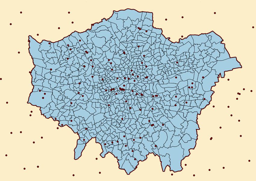
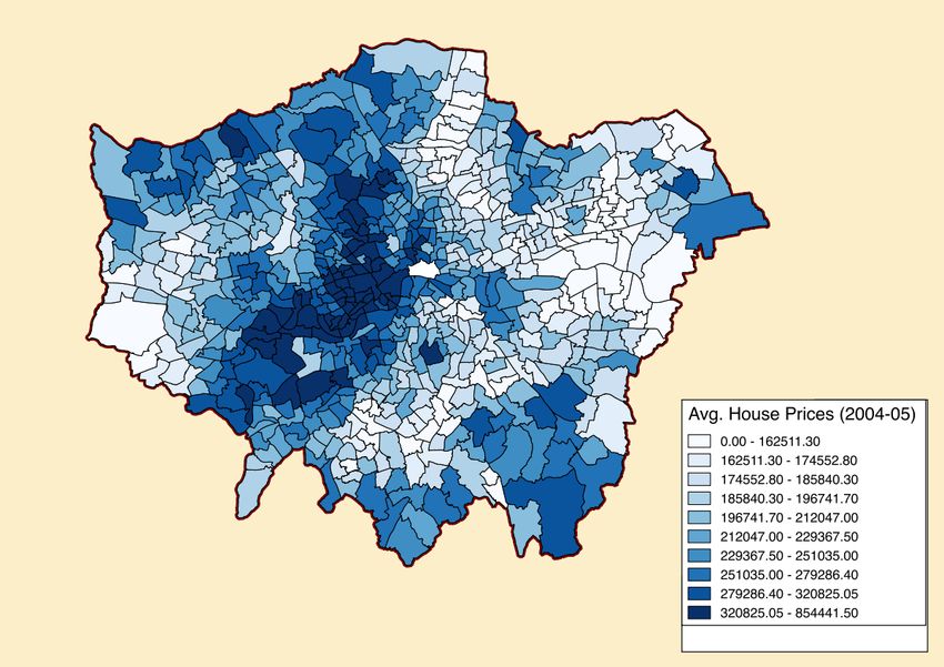
To examine these aspects, we stratify our sample of 624 wards according to their
average house price as a proxy for income (Figure 7). In figure 8, we plot the point estimates
and corresponding 95% confidence interval for each decile. We also include the long term
average AQI levels for each decile and find that long term pollution concentrations tends to be
larger in wards with higher average house prices. Overall, we find a U-shape relationship where
the larger effects seems to occur at the tails of the distribution. This suggests that both dynamics
which we described above might be at play at our spatial scale of measurement: (1) the
estimated effect of pollution on crime is larger in wealthier wards which are exposed to higher
pollution levels and (2) despite relatively low exposure, the effect of pollution on crime is also
large in the poorest wards.
VI. The Underlying Mechanism
Our results so far support our initial hypothesis that altered behaviour under heightened
pollution exposure results in a larger number of crimes committed. In this section we will
leverage our rational choice framework to uncover the underlying mechanism for our empirical
findings. More specifically, in section 2 we outlined that within the rational choice framework
of crime, the effect of pollution on crime may be mediated through the following three
channels: (i) the payoff from crime %"& increases relative to the cost of future punishment )"&
which is discounted at the rate (, (ii) the probability of being punished !" is lowered, or (iii)
the potential offender’s preferences $" . become more risk accepting. We will now explore
these channels in more detail.
26
For a full discussion on this subject see Hsiang et al. (2017).
17Risk perception and risk preferences:
Changes that lead to more risk taking should be expected to also lead to more criminal
offences. In the expected utility framework presented above, more risk taking and hence more
crime, can result from changes in either risk preferences or in risk perceptions. Existing
evidence does not support changes in risk perception or risk preferences as an explanation for
the observed effect of air pollution on crime. To explain an increase in crime, elevated levels
of air pollution should be linked to a more optimistic evaluation of ones odds of getting away
with a crime unpunished (lower p1 ) or a change towards more risk loving preferences (higher
U′′1 . ).
While the existing empirical evidence on air pollution and risk taking is limited, it
suggests an association in the opposite direction. Heyes et al. (2016) provide suggestive
evidence that risk taking in financial markets is lower on days with elevated levels of air
pollution. However, one may doubt the relevance of the behaviour of investment professionals
for the understanding of criminal activity. We thus perform an additional test, the results of
which support a negative association between risk taking and air pollution. More specifically,
we use weekly data on national lottery sales in England and Wales from (draws on Wednesday
and Saturday of each week) for a rudimentary assessment of the link between risk taking and
air pollution27. We find that a 10 point increase in the national average AQI on the day of a
draw is associated with a 1.5% decrease in lottery sales accounting for weather conditions, day
of the week, month and year of the draw.
Finally, a negative association between air pollution and risk taking is in line with the
medical literature. Experimental evidence documents that, if anything, subjects become more
risk averse when administered the stress hormone cortisol (Kandasamy et al., 2014) or when
27
We use data on Main Sales (Saturday and Wednesday) in the UK National Lottery as collected by http://lottery.merseyworld.com. We run
various specifications at times including weather controls (temperature, relative humidity, their interaction, wind speed and precipitation) as
well as fixed effects for Saturday/Wednesday draws, the month and the year of the draw. Data cover all weeks in 2009-2014. The full set of
results from our lottery analysis is available upon request.
18exposed to physical stress (Porcelli and Delgado, 2009). As we discuss further below, acute
exposure to air pollution has been linked to elevated levels of cortisol (Li et al., 2017). We
would consequently expect to result in individuals becoming more risk averse when exposed
to higher levels of pollution. In sum, both existing empirical evidence and our rudimentary
analysis using lottery sales suggest that if anything air pollution may reduce risk taking
behaviour and thus is unlikely to explain the observed increase in criminal activity on polluted
days.
Perceived payoff vs. punishment: The potential role of discounting
If we wish to maintain the rational choice framework outlined above, and by the
principle of exclusion, our results suggest that the increase in criminal activity may be driven
by changes in the perceived gain relative to the punishment. Such a change in the perceived
costs and benefits of a criminal offence can be driven by two changes – an increase in the
perceived benefit (%"& ), or a decrease in the perceived cost ()"& ) discounted at the rate (,
A first channel through which pollution may affect crime is by increasing the perceived
benefit (%"& ). While it is plausible that heightened aggression (or similar effects on emotional
disposition) might drive an increase in perceived benefit of interpersonal crime, it seems
unlikely that altered emotional disposition affects the perceived benefit of crimes that are
economically motivated and often committed by “professional” criminals. For example, we
would not expect the emotional disposition of a pickpocket to significantly alter her expected
gain from theft. We find that pollution drives most types of crimes (Figure 5), not only those
which are interpersonal but also those which are more economically motivated28. Therefore,
28
This is in line with a recent paper in the psychology literature, which finds an association between air
pollution and a wide range of crimes in the United States (Lu et al., forthcoming).
19we conclude that an increase in the perceived benefit (%"& ) of crime is not consistent with our
findings.
Whilst we do not expect air pollution today to influence sentencing ()"& ) which occurs
in the future, there is evidence from the medical literature which suggests that air pollution
exposure may alter the relative perceived costs of punishment by raising the effective discount
rate (β) applied to the future prospect of punishment. Acute exposure to elevated levels of air
pollution has been linked to heightened concentration of stress hormones. In a rare
experimental study, Li et al. (2017) provide evidence that acute exposure to elevated levels of
PM2.529 leads to significant increases in cortisol (hydrocortisone), cortisone, epinephrine, and
norepinephrine. Changes in blood levels of stress hormones are in turn expected to result in
behavioural change. More specifically, heightened concentrations of stress hormones,
especially cortisol, have been shown to alter time-preferences. In a controlled experiment, Riis-
Vestergaard et al. (2018) find that subjects that were administered cortisol 15 minutes before
the experimental task exhibited a strongly increased preference for small immediate rewards
relative to larger but delayed rewards. The same was found in studies that randomly assigned
physical stress rather than administering stress hormones. Again, individuals subject to
physical stress (or pain) exhibited greater impatience than relevant control groups (Delaney et
al., 2014; Koppel et al., 2017). In sum, acute exposure to elevated levels of air pollution
(PM2.5) may temporarily increase the discount rate applied to intertemporal trade-offs via its
effect on blood levels of stress hormones. Increased discounting lowers the cost associated with
potential future punishment ()"& ) and consequently results in an increase in criminal offences.
Increased discounting also has the potential to reconcile the increase in crime (where potential
29
Li et al. (2017) conduct a randomised, double-blind crossover trial where subjects (college students) have air purifiers installed in their
dormitories for a period of 9 days. Some purifiers are functioning (mean PM2.5 exposure of 24 mg/m3), others are not (mean PM2.5
exposure of 53 mg/m3).
20future punishment is discounted relative to immediate gains) with the observed decrease in
lottery sales (where potential future winnings are discounted relative to immediate ticket costs).
VII. Conclusion
This paper investigates the potential link between ambient air pollution and crime.
Using two separate identification strategies, we find that daily variation in air pollution is
positively linked to higher crime rates in London. We also find that pollution affects most
crime types but appears to have larger effects on crimes which are less severe. Based on the
rational choice model and our empirical results, we conclude that the underlying channel for
our findings is likely to be higher discounting of future punishment on high pollution days.
Finally, we investigate whether our estimates vary across resident income groups and find a U-
shape relationship where the larger effects seem to occur at the tails of the distribution.
Our results provide evidence that environmental factors are an important determinant
of crime. Whilst previous studies focused on weather conditions, which are unlikely to be
shaped by policymakers, we have studied an environmental condition which can be regulated.
Our results suggest that improving air quality in urban areas by tighter environmental policy
may provide a cost effective way to reduce crime. Furthermore, our results are present at levels
which are well below current US Environmental Protection Agency (EPA) and UK Department
for Environment, Food & Rural Affairs (DEFRA) standards which further suggest that it may
be economically beneficial to lower existing guidelines. Finally, given the link between air
pollution and crime, our results therefore suggest that examining the effects of air pollution on
health impacts alone, may lead to a substantial underestimation of its societal costs.
21References
Anderson, M.L. (2015). As The Wind Blows: The Effects of Long-Term Exposure to Air
Pollution on Mortality. NBER Working Paper No. 21578. National Bureau of Economic
Research.
Becker, G. (1968). Crime and punishment: An economic approach. In The economic
dimensions of crime, 13-68. Palgrave Macmillan, London.
Burke, M., Hsiang, S.M. and E. Miguel (2015). Climate and Conflict. Annual Review of
Economics, 7, 577-617.
Chay, K. Y., & Greenstone, M. (2003). The impact of air pollution on infant mortality:
evidence from geographic variation in pollution shocks induced by a recession. The quarterly
journal of economics, 118(3), 1121-1167.
Cohen, F., & Gonzalez, F. (2018). Understanding interpersonal violence: the impact of
temperatures in Mexico (No. 291). Grantham Research Institute on Climate Change and the
Environment.
Delaney, L., Fink, G. and C. Harmon (2014). Effects of Stress on Economic Decision-Making:
Evidence from Laboratory Experiments. Discussion Paper No. 8060, IZA.
Deryugina, T., Heutel, G., Miller, N. H., Molitor, D., & Reif, J. (2016). The mortality and
medical costs of air pollution: Evidence from changes in wind direction (No. w22796).
National Bureau of Economic Research.
Department for Environment, Food and Rural Affairs (2017). Automatic Urban and Rural
Network. Data retrieved 26th November 2017 at https://uk-air.defra.gov.uk/data/data_selector.
Dockery, D. W., Pope, C. A., Xu, X., Spengler, J. D., Ware, J. H., Fay, M. E., ... & Speizer, F.
E. (1993). An association between air pollution and mortality in six US cities. New England
journal of medicine, 329(24), 1753-1759.
Draca, M., Machin, S., & Witt, R. (2011). Panic on the streets of london: Police, crime, and the
july 2005 terror attacks. American Economic Review, 101(5), 2157-81.
Ebenstein, A., Lavy, V., & Roth, S. (2016). The long-run economic consequences of high-
stakes examinations: evidence from transitory variation in pollution. American Economic
Journal: Applied Economics, 8(4), 36-65.
Ehrlich, I. (1973). Participation in Illegitimate Activities: A Theoretical and Empirical
Investigation. Journal of Political Economy, 81(3), 521-565.
Graff Zivin, J., & Neidell, M. (2012). The impact of pollution on worker
productivity. American Economic Review, 102(7), 3652-73.
Heyes, A., Neidell, M. and S. Saberian (2016). The Effect of Air Pollution on Investor
Behavior: Evidence from the S&P 500. NBER Working Paper No. 22753. National Bureau of
Economic Research.
22Herrnstadt, E., Heyes, A., Muehlegger, E., & Saberian, S. (2016). Air pollution as a cause of
violent crime: Evidence from Los Angeles and Chicago. Technical Report, mimeo.
Hsiang, S., Oliva, P., & Walker, R. (2017). The distribution of environmental damages (No.
w23882). National Bureau of Economic Research.
Koppel, L., Andersson, D., Morrison, I., Posadzy, K., Västfjäll, D. and G. Tinghög (2017). The
effect of acute pain on risky and intertemporal choice. Experimental Economics, 20, 878-893.
Land Registry, HM (2017). Average house prices by borough, ward, MSOA, LSOA & postcode.
Data retrieved 13th December 2017 at https://data.london.gov.uk/dataset/average-house-prices.
Li, H., Cai, J., Chen, R., Zhao, Z., Ying, Z., Wang, L., ... & Kan, H. (2017). Particulate matter
exposure and stress hormone levels: a randomized, double-blind, crossover trial of air
purification. Circulation, 136(7), 618-627.
Lichter, A., Pestel, N., & Sommer, E. (2017). Productivity effects of air pollution: Evidence
from professional soccer. Labour Economics, 48, 54-66.
Logan, W. P. D. (1953). Mortality in the London fog incident, 1952. The Lancet, 261(6755),
336-338.
Lu, J.G., Lee, J.L., Gino, F., & Galinsky, A.D. (forthcoming). Polluted morality: Air pollution
predicts criminal activity and unethical behavior. Pyschological Science, forthcoming.
Machin, S., Marie, O., & Vujić, S. (2011). The crime reducing effect of education. The
Economic Journal, 121(552), 463-484.
Met Office (2012). Met Office Integrated Data Archive System (MIDAS) Land and Marine
Surface Stations Data (1853-current). NCAS British Atmospheric Data Centre. Data retrieved
23rd November 2017, http://catalogue.ceda.ac.uk/uuid/220a65615218d5c9cc9e4785a3234bd0.
Neidell, M. (2017). Air pollution and worker productivity. IZA World of Labor.
Pope 3rd, C. A., Bates, D. V., & Raizenne, M. E. (1995). Health effects of particulate air
pollution: time for reassessment?. Environmental health perspectives, 103(5), 472.
Ranson, M. (2014). Crime, weather, and climate change. Journal of Environmental Economics
and Management, 67(3), 274-302.
Reyes, J. W. (2007). Environmental policy as social policy? The impact of childhood lead
exposure on crime. The BE Journal of Economic Analysis & Policy, 7(1).
Reyes, J. W. (2015). Lead exposure and behavior: Effects on antisocial and risky behavior
among children and adolescents. Economic Inquiry, 53(3), 1580-1605.
Riis-Vestergaard, M.I., van Ast, V., Cornelisse, S., Joels, M. and J. Haushofer (2018). The
effect of hydrocortisone administration on intertemporal choice. Psychoneuroendocrinology,
88, 173-182.
23Sager, L. (2016). Estimating the effect of air pollution on road safety using atmospheric
temperature inversions. Grantham Research Institute on Climate Change and the Environment
working paper, 251.
Schlenker, W., & Walker, W. R. (2015). Airports, air pollution, and contemporaneous
health. The Review of Economic Studies, 83(2), 768-809.
Ward Atlas (2017). Ward Profiles and Atlas. Data retrieved 7th December 2017 at
https://data.london.gov.uk/dataset/ward-profiles-and-atlas.
http://www.independent.co.uk/news/uk/politics/sadiq-khan-crime-weak-causes-violence-
london-met-police-theresa-may-home-office-stabbings-murders-a8141436.html
24Table 1
Descriptive Statistics
By House Prices
All Low High
Variable (1) (2) (3)
Crime (log) 1.39 1.43 1.36
(0.67) (0.64) (0.70)
Crime (# per 100k population) 34.06 32.73 35.38
(38.43) (24.93) (48.25)
Air Quality Index 30.06 28.51 31.60
(AQI) (9.177) (8.060) (9.934)
28.05 26.70 29.40
PM10
(10.35) (9.863) (10.65)
50.00 46.11 53.90
Nitrogen Dioxide
(21.06) (18.15) (22.96)
4.710 4.667 4.752
Sulfur Dioxide
(3.492) (3.600) (3.380)
33.17 33.94 32.39
Ozone
(17.86) (17.81) (17.86)
Temperature 11.76 11.86 11.67
(5.805) (5.763) (5.844)
76.63 75.51 77.75
Relative Humidity
(11.42) (11.46) (11.28)
7.588 7.435 7.741
Wind Speed
(4.036) (3.712) (4.330)
1.581 1.497 1.670
Rainfall
(3.526) (3.261) (3.786)
0.0506 0.0497 0.0514
Unemployment
(0.0155) (0.0152) (0.0158)
1.677 1.721 1.632
Tube activity (million # per week)
(2.248) (2.304) (2.190)
0.527 0.469 0.585
Police deployment (log)
(0.379) (0.293) 0.441
Observations 455520 227760 227760
Notes: Standard deviations are in parentheses. Each observation corresponds to one of 730 days and one of 624 wards. Data as described in the text from the following sources: Air pollution data from DEFRA (2017), weather conditions from
the Met Office (2012), house prices from HM Land Registry (2017), and crime data from Draca et al. (2011).
25Table 2
Pooled OLS and Fixed Effect Models of Air Pollution's Impact on Crime
Polled OLS Fixed Effects
(1) (2) (3) (4) (5) (6)
AQI (10 units) 0.064*** 0.029*** 0.020*** 0.009*** 0.009*** 0.457***
(0.0124) (0.0101) (0.0041) (0.0025) (0.0025) (0.1134)
Controls N Y Y Y Y Y
Ward FE N N Y Y Y Y
DOW FE N N N Y Y Y
Year-Month FE N N N N Y Y
R-squared 0.007 0.060 0.372 0.383 0.385 0.688
Observations 419,210 398,437 398,437 398,437 398,437 433,277
Notes: Each column in the table represents a separate regression. In column (1)-(5), the dependent variable is the (log) number of criminal offences per day and ward and in column (6) the dependent variable is the crime rate per
100,000 people. AQI is based on air pollution readings from the three closest AURN monitoring stations (weighted by inverse squared distance). Control variables include weather characteristics (temperature, relative humidity and
wind speed),ward-level police deployment and unemployment levels. Standard errors are cluster-robust in two dimensions, over wards and dates. * pTable 3
Air Pollution's Impact on Crime
Polled OLS Fixed Effects
No Controls Controls No Controls Controls
(1) (2) (3) (4)
Dummy for AQI >20 & 25 & 30 & 35 0.177*** 0.035 0.083*** 0.028***
(0.0279) (0.0241) (0.0142) (0.0077)
Observations 419,210 398,437 419,210 398,437
Notes : See Table 2. Each column in the table represents a separate regression.
27Table 4
Instrumental Variable Models of Air Pollution's Impact on Crime
OLS 2SLS
(1) (2) (3) (4) (5) (6)
AQI (instrumnetd) 0.009*** 0.009*** 0.127*** 0.018** 0.039*** 0.017**
(0.0025) (0.0025) (0.0361) (0.0083) (0.0141) (0.0084)
Controls Y Y Y Y Y Y
Ward FE Y Y N Y Y Y
DOW FE Y Y N Y N Y
Year-Month FE Y Y N N Y Y
First stage (F-test) 22.91 13.69 13.25 13.54
Observations 398,437 396,521 396,521 396,521 396,521 396,521
Notes : See Table 2. Columns (3)-(6) instrumental variable estimates.
28Table 5
Measuring the Relationship between Crime and Air Pollution on the Actual Day and Irrelevant Days
Pooled OLS Fixed Effects
No Controls Controls No Controls Controls
(1) (2) (3) (4)
Day of Crime 0.062*** 0.027*** 0.022*** 0.009***
(0.0120) (0.0095) (0.0043) (0.0024)
Previous Week 0.050*** 0.017** 0.006 -0.001
(0.0122) (0.0085) (0.0043) (0.0023)
Previous Month 0.038*** -0.001 -0.010** -0.002
(0.0119) (0.0085) (0.0041) (0.0023)
Previous Year 0.041*** 0.003 -0.002 -0.001
(0.0127) (0.0094) (0.0055) (0.0032)
Notes : See Table 2. Each column in the table represents a separate regression.
29You can also read