INSTITUT F UR INFORMATIK - der Ludwig-Maximilians-Universit at M unchen
←
→
Page content transcription
If your browser does not render page correctly, please read the page content below
INSTITUT FÜR INFORMATIK
der Ludwig-Maximilians-Universität München

H OW     WELL DOES A CROWD
 RECOGNIZE DIFFERENCES
BETWEEN PHOTOGRAPHS OF
   THE SAME ARTWORKS ?

           Cedric Kummer

                 Bachelorarbeit
       Aufgabensteller   Prof. Dr. François Bry
       Betreuer          Prof. Dr. François Bry,
                         M.Sc. Stefanie Schneider

       Abgabe am         26.04.2021
Erklärung

Hiermit versichere ich, dass ich die vorliegende Arbeit selbständig verfasst habe und
keine anderen als die angegebenen Hilfsmittel verwendet habe.

                                                                  C. kümmer
München, den 26.04.2021                                                   Cedric Kummer
Matrikelnummer:                                                                   11565365

                                             i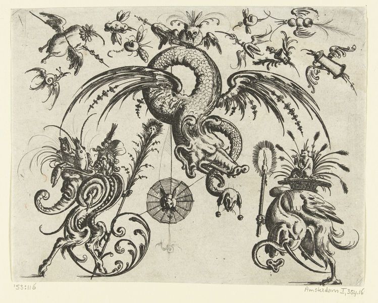
Abstract

This bachelor thesis presents two novel algorithms that can be used in combination to de-
termine the similarity of two photographs. The one algorithm analyses and compares the
tags of two reproductions. These tags were assigned in advance, mainly by laypersons
on the ARTigo platform. More precisely, the algorithm calculates the cosine similarity of
the tags that have been assigned to the images. The information provided by the first al-
gorithm can then be used to verify how much the tags annotated by the crowd differ be-
tween two reproductions that are already known to represent the same original. The AR-
Tigo platform is part of an interdisciplinary project within the field of digital art studies,
in which computer scientists and art history scholars conduct joint research. This bache-
lor thesis is part of that research project. The second algorithm is a computer vision algo-
rithm that first calculates the feature vectors of the images. These are then matched so as
to estimate how similar the two images are. Then, in a second step, the second algorithm
calculates the general colour difference of the images in the Lab colour space. The results
of the second algorithm can then be used to draw conclusions about the actual difference
between the images. These results can also be used to classify whether, in the case of a
high degree of similarity between the tags, two digital reproductions of the same origi-
nal are involved, or whether both reproductions merely show the same or a similar motif.
Finally, the thesis reports how the similarity of the assigned tags and the results of com-
puter vision can be used to draw conclusions regarding whether two images represent the
same original. This thesis is concluded with reflections on further possible application of
the approach described in this thesis as well as how the work reported about in this thesis
could be deepened.

                                              ii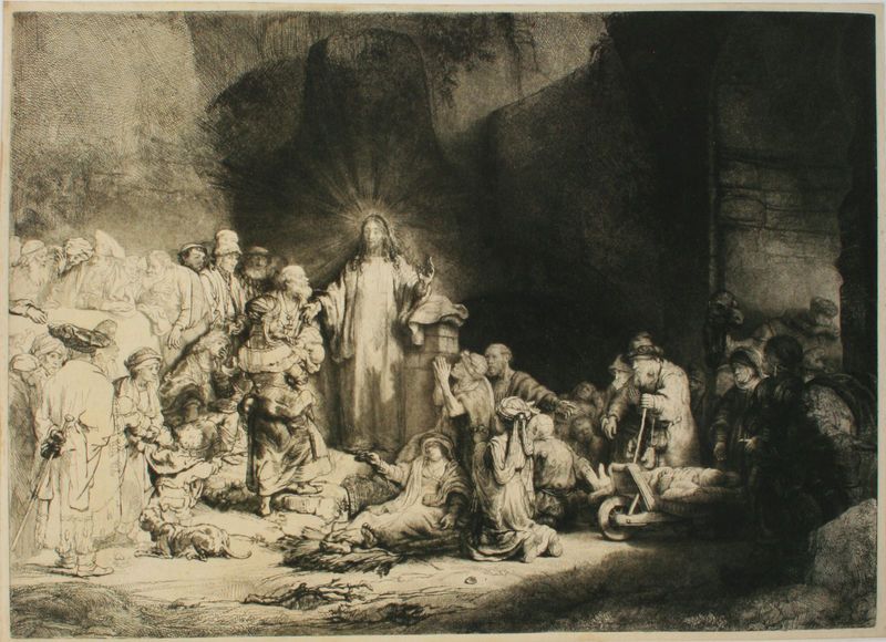
Acknowledgments

I would like to thank Professor François Bry and Stefanie Schneider very much for their
excellent supervision during this bachelor thesis. Unfortunately, due to the still ongoing
pandemic, we were never able to meet in person, except via Zoom. I would also like to
thank my family and friends who have always supported me where they could during
this time. I was able to learn a lot of things during this time, from data analysis in R to
image processing with OpenCV and to the process of scientific work.

                                             iii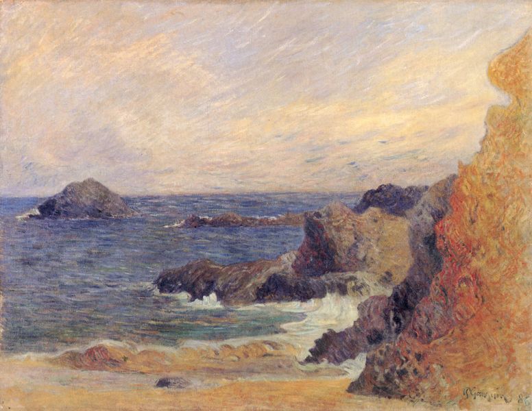
Contents

1   Introduction                                                                                                                                  1

2   ARTigo                                                                                                                                         6
    2.1 What are social tags and why are they used by ARTigo? . . . . . . . . . . . . .                                                            6
    2.2 Data creation on an example . . . . . . . . . . . . . . . . . . . . . . . . . . . . .                                                      7
    2.3 Data structure . . . . . . . . . . . . . . . . . . . . . . . . . . . . . . . . . . . . .                                                   7

3   Related Work                                                                                                                                  9

4   Cleansing the ARTigo dataset                                                               11
    4.1 Merging and cleansing the data . . . . . . . . . . . . . . . . . . . . . . . . . . . 11
    4.2 Correcting misspelled tags . . . . . . . . . . . . . . . . . . . . . . . . . . . . . . 12

5   Data Analysis                                                                                                                                 15
    5.1 Creation of the sparseMatrix . . . . . . . . . . . . . . . . . . . . . . . . . . . . .                                                    15
    5.2 Computing the cosine similarity . . . . . . . . . . . . . . . . . . . . . . . . . .                                                       16
    5.3 Evaluation of the calculated cosine similarities . . . . . . . . . . . . . . . . . .                                                      17

6   Computer Vision                                                                                                                               25
    6.1 Feature detection . . . . . . . . . . . .     .   .   .   .   .   .   .   .   .   .   .   .   .   .   .   .   .   .   .   .   .   .   .   25
        6.1.1 Computing the features . . . .          .   .   .   .   .   .   .   .   .   .   .   .   .   .   .   .   .   .   .   .   .   .   .   26
        6.1.2 Comparing the features . . . .          .   .   .   .   .   .   .   .   .   .   .   .   .   .   .   .   .   .   .   .   .   .   .   27
    6.2 Computation of the colour differences         .   .   .   .   .   .   .   .   .   .   .   .   .   .   .   .   .   .   .   .   .   .   .   28
    6.3 Results . . . . . . . . . . . . . . . . . .   .   .   .   .   .   .   .   .   .   .   .   .   .   .   .   .   .   .   .   .   .   .   .   34

7   Conclusion                                                                                  43
    7.1 Evaluation of the results . . . . . . . . . . . . . . . . . . . . . . . . . . . . . . . 43
    7.2 Further thoughts . . . . . . . . . . . . . . . . . . . . . . . . . . . . . . . . . . . 44

Bibliography                                                                                                                                      45

                                                 iv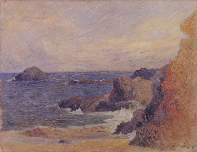
CHAPTER          1

                                                                          Introduction

Duplicates in image databases are not uncommon. There are often several scans or pho-
tographs of one and the same work of art. Filtering reproductions of the same original
from these databases is a very resource-intensive task. Several employees have to sift
through all the material and then decide which reproductions show the same original.
The ARTigo project at Ludwig Maximilians Universität Munich uses a large number of
users to categorise these images using so-called social tags mainly assigned by layper-
sons.
The question arises whether the differences between the reproductions are reflected in
the tags. Furthermore, the question arises whether, if very similar tags are assigned to dif-
ferent reproductions, this can also be used to identify reproductions that show the same
original.
In the scope of this bachelor thesis, an algorithm was developed which determines whether
two reproductions represent the same original by comparing the tags assigned to them.
For this purpose, a small subsample of the ARTigo database was used, which only con-
tains reproductions of which it is already known that they show the same original. The
tags of each reproduction are first generalised to make them more comparable. For this
purpose, the Levenshtein neighbours of each tag that has been assigned to a resource are
determined. A spelling check is then performed on these neighbours. The frequencies of
the other tags are then summed up with the frequency with which the correctly spelled
tag was assigned to the resource. This filters out any typos or misspellings and eventu-
ally makes it easier to compare the tags of the resources. Afterwards, a matrix is formed
which contains all reproductions and tags. The values of the matrix are the frequencies
with which a tag has been assigned to a reproduction. A principal component analysis
is then applied to this matrix. The result of this is then multiplied by the original matrix.
Finally, the cosine distance of the reproductions to each other is determined.
Since it is already known which reproductions portray the same original, a high match
value is to be expected for these. After this analysis, a computer vision algorithm deter-
mines to what extent the reproductions actually differ. Ideally, the algorithm confirms the
results of the data analysis.
This algorithm, in combination with the ARTigo game, saves researchers from having to
filter the reproductions by hand and validate whether they represent the same original.
Applied to the entire dataset of the ARTigo project, the algorithm could identify those
reproductions that represent the same original based on the similarity of their tags. The

                                             1
CHAPTER 1. INTRODUCTION                                                                           2

researchers only have to decide in the last instance which of the two reproductions can be
removed from the database.
The following figures each show two pictures of which it is already known that they rep-
resent the same original.

(a) Katsushika Hokusai, Der sieben Ri lange        (b) Katsushika Hokusai, Der sieben Ri lange
Strand von Soshu, Blatt 13 aus der Serie: 36       Strand von Soshu, Blatt 13 aus der Serie: 36
Ansichten des Fuji, Museum für Kunst und          Ansichten des Fuji, Museum für Kunst und
Gewerbe Hamburg - 1830 [15]                        Gewerbe Hamburg - 1830-1831 [16]

            Figure 1.1: Two different woodblock prints showing the same motif

These two woodblock prints by Katsushika Kokusai, which can be seen in Figure 1.1,
show the same motif, but the horizon of the two pictures differs. The details in these im-
ages are not too high. Therefore, it can be expected that rather few different tags have
been assigned to the two images. The problem with these two reproductions, however,
is that this is a false positive assignment. However, it is not expected that this difference
will be detected by the computer vision algorithm.

(a) Paul Gauguin, Felsige Meerküste, Göteborgs   (b) Paul Gauguin, Rochers au bord de la mer,
Konstmuseum - 1886 [21]                            Göteborgs Konstmuseum - 1886 [22]

   Figure 1.2: Two reproductions showing the same original but differing in brightness

In Figure 1.2 one can clearly see two different photographs of the artwork ”Rocky Sea
Coast” by Paul Gauguin. Since the level of detail of the two images is not great, very sim-
ilar tags are to be expected. The computer vision algorithm should detect that the two
images show the same original, with the right image being considerably darker than the
left.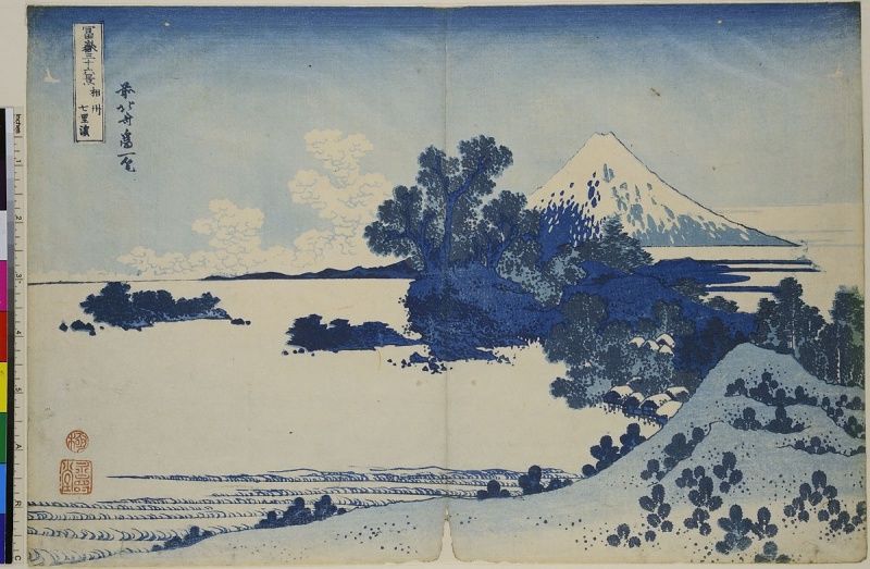
CHAPTER 1. INTRODUCTION                                                                          3

(a) Wenzel Hollar, Ansicht von Köln und Deutz   (b) Wenzel Hollar, Vogelansicht von Köln und
aus der Vogelschau, Stadtmuseum Köln - 1635     Deutz, Staatliche Kunsthalle Karlsruhe - un-
[39]                                             known [40]

              Figure 1.3: Two copper engravings depicting the same original

The two copperplate engravings by Wenzel Hollar, which can be seen in Figure 1.3, have
a very high level of detail, it is to be expected that many different tags have been assigned
to them. It is therefore to be expected that the tag similarity of the two images will not
be that high. The computer vision algorithm should recognise that the two images are
two reproductions from the same original. It should also recognise that the right image is
slightly brighter than the left.

(a) Rembrandt, Christus heilt die Kranken,
                                                 (b) Rembrandt, Das Hundertguldenblatt, Al-
genannt das Hundertguldenblatt, Staatliche
                                                 bertina Wien - 1647-1649 [27]
Kunsthalle Karlsruhe - 1601-1649 [26]

                     Figure 1.4: Different executions of the same theme

The two reproductions in Figure 1.4 both show Rembrandt’s ”Hundred Guilder Leaf ”. They
differ greatly in their contrast, brightness and general colouring. However, since a very
familiar scene is depicted here, it is quite reasonable to assume that the tags assigned will
be quite similar. However, the computer vision algorithm should be able to detect a clear
difference here.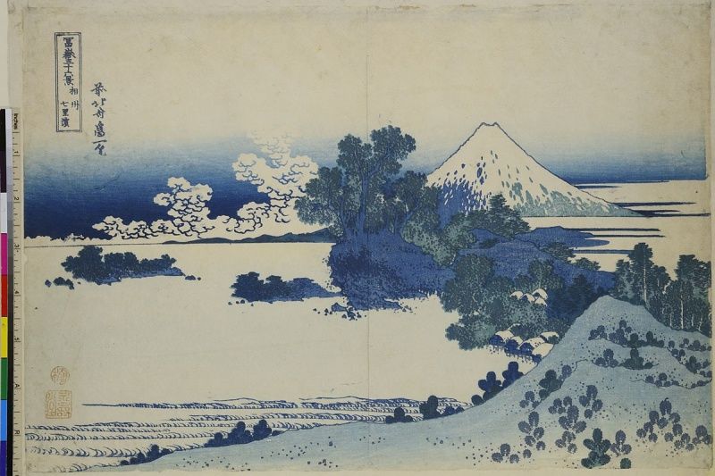
CHAPTER 1. INTRODUCTION                                                                         4

(a) Bartolomé Esteban Murillo, Einladung zum     (b) Bartolomé Esteban Murillo, Einladung zum
Pelota - Spiel, The trustees of Dulwich Picture   Pelota - Spiel, The Trustees of Dulwich Picture
Gallery London - 1670 [3]                         Gallery London - 1670 [4]

                 Figure 1.5: Two reproductions that differ in their colouring

The two reproductions of the artwork ”Invitation to the Pelota - Game” by Bartolomé Este-
ban Murillo in Figure 1.5 differ clearly in their colouring. The left image has a clear yel-
low/red cast. In general, quite similar tags are to be expected. The computer vision algo-
rithm should be able to show clear differences.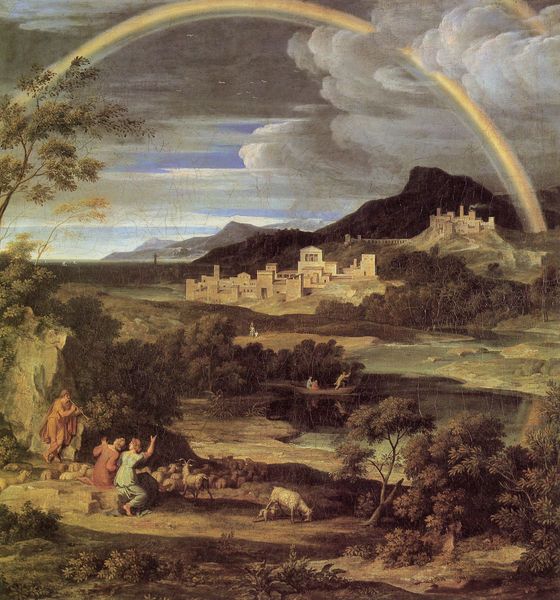
CHAPTER 1. INTRODUCTION                                                                         5

                                                 (b) Utagawa Hiroshige, 100 berühmte An-
(a) Utagawa Hiroshige, Die Komagata-Halle
                                                 sichten von Edo, Institution not known 1856-
und die Azuma-Brücke, Blatt 62 aus der Serie:
                                                 1858 [33]
100 berühmte Ansichten von Edo, Museum für
Kunst und Gewerbe Hamburg - 1857 [34]

            Figure 1.6: Two different woodblock prints showing the same motif

These two reproductions, shown in Figure 1.6 made by Utagawa Hiroshige, both from the
series ”100 famous views of Edo”, are clearly two different woodblock prints. Since there
is a significant difference in colour, it is to be expected that these differences will also be
reflected in the tags annotated by the crowd.

In the following chapter, the ARTigo project is introduced. It also illustrates how the data
set used in this bachelor thesis has been created.
The following chapter presents some of the work and tools that were necessary to make
this thesis possible.
Chapter 4 shows which data was selected as a basis for the algorithm. It also explains
why these data was chosen and why it had to be cleansed again.
Chapter 5 then describes how the existing data has been analysed and how the algorithm
decides which reproductions represent the same original.
Chapter 6 then follows with the colour subtraction of the images. This is done because it
is possible to quantify how good the analysis or even the assignment of the tags was.
Finally, there is an outlook on what could not be realised in this thesis due to time con-
straints, but which can help the developed algorithm to become even more accurate. In
addition, there is an outlook on what this algorithm could be used for.
CHAPTER 2
ARTigo
The ARTigo project [24] at LMU Munich, an interdisciplnar project of the Institutes for Art
History and for Informatics, uses various games which allow the user to playfully partic-
ipate in art history. One of the games shares its name with the project and web gaming
platform. In ARTigo, two players are randomly selected. They are then shown 5 repro-
ductions of a work of art, which can be a scan or a photograph, for example. These re-
productions are randomly selected initially from the Artemis image database of the Lud-
wig Maximilians Universität Munich. By the time other image databases joined ARTigo.
Among them for example the one of ”Rijksmuseum”. The image database of the ”Mu-
seum für Kunst und Gewerbe Hamburg”, for example, was added through a cooperation.
For each picture, one has 60 seconds to annotate the features he is seeing. Both players
gain points for each identical tag. It is therefore advisable to annotate the most prominent
features of the picture in order to collect as many points as possible. ARTigo relies on so-
called social tags, the reason for this being useful in art history is explained in the next
section. The method used in ARTigo is based on that of Luis von Ahn, who developed
a game 1 that makes it possible to transfer the involvement of laypersons in the creation
process so successfully practised in the online encyclopaedia Wikipedia to the field of im-
age annotation while at the same time controlling misuse. [9]
In each run, the players get to see five pictures. For each picture, they have one minute to
enter keywords that they recognise in the picture and that they think the other player also
recognises. So the limited time puts them under some time pressure. Among other things,
this is also reflected in the typos of some tags. The challenges that come along with this
are discussed in chapter 4.
2.1 What are social tags and why are they used by ARTigo?
Social tagging refers to the free, i.e. arbitrary, assignment of keywords (tags) by a group
of people, whereby they explicitly do not have to be experts. The tags assigned in each
case are aggregated and thus form a keyword index.[1] The great advantage of social tag-
ging is therefore that the tagging is done by a large interdisciplinary crowd. This group
consists mainly of laypersons, in the case of ARTigo precisely not of studied art scholars.
1 http://www.gwap.com/gwap/gamesPreview/espgame/
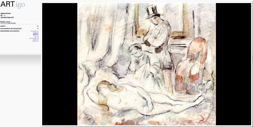
6CHAPTER 2. ARTIGO 7 Although this does not mean that there are no experts to be found in this group. ARTigo uses these social tags without quality control of the input. Players can freely choose any number of terms to describe a picture. Thus, both form aspects and semantic content aspects can appear in the created keyword catalogue.[9] 2.2 Data creation on an example In Figure 2.1 you can see a running ARTigo game. Shown directly below the picture is a text field in which the player enters the tag he can recognise in the picture. Once he has entered the tag, he presses the button next to it to assign the word respectively these words to the picture. At the left edge the player can see which terms he has entered and how many points he has received for them. If the entered tag does not yet exist in the database, a new one is created and a new entry is created in the Tagging relation, which receives this new tag, this image and the number 1 as the frequency for the first time. If the entered tag already exists, the tagging relation is checked to see if this tag has al- ready been assigned to this image. If this is the case, the frequency of this entry in the database is increased by one. If this is not the case, a new entry is created in the tagging relation as described above. Above the word list, the player can see the time he has left to assign more tags to this pic- ture. Figure 2.1: A running ARTigo game (Image: Paul Cézanne, Olympia, 1875/1877, New York (New York), Collection Stern) 2.3 Data structure As already mentioned in the previous section, the tags that a player gives to an image are stored in a database. The frequency with which these tags have been assigned to a partic- ular resource is essential for this thesis, as the algorithm that has been developed needs to know the frequency with which a particular tag has been assigned to a particular re- source. This information can then be used to decide how well the tags of two resources match. The ARTigo data model (Figure 2.2) used for this thesis is engineered as follows:
CHAPTER 2. ARTIGO                                                                            8

Tag:
This relation reflects an actually assigned tag. This tag can be identified by a unique id.
Name describes exactly the word that was entered by a player. Language gives informa-
tion about the language in which the tag was written. In addition to German, English and
French are also available.
Artist:
This relation contains all the different artists who can be assigned to their artworks on the
basis of their id.
Resource:
Describes an image from the database. Id again stands for the unique identification num-
ber. The remaining part contains further information about the painting, which is not rele-
vant for this thesis.
Tagging:
This relation contains the actual assignments of a tag to a resource and the frequency of
annotation. Resource id refers to the image and tag id to the assigned tag. Frequency de-
scribes how often this tag has been assigned to this image.
Relation:
There are two images here which are knowingly reproductions of the same original. The
entry in the type field is also important. This can either be ”variant of” or ”part of”. In the
case of variant of, the two images differ in colouring, contrast, brightness or similar. In the
case of part of, one of the pictures only shows a section of what can be seen in the other
picture.

                    Figure 2.2: ER diagram of the 2018 data structure [5]
CHAPTER 3
Related Work
In her article ”Social tagging als Methode zur Optimierung kunsthistorischer Bilddatenbanken–
eine empirische Analyse des ARTigo-Projekts” [9], Laura Commare writes about how the
ARTigo project uses social tags to help ensure that images in a database are tagged with
high quality by a large group of art experts and laypeople. Based on this article, it can be
assumed that it is possible to develop an algorithm that can eventually group reproduc-
tions that show the same original based on the tags used.
In their article ”The Computer as Filter Machine: A Clustering Approach to Categorize Artworks
Based on a Social Tagging Network” [32], Stefanie Schneider and Hubertus Kohle present
the application of a clustering algorithm that uses crowdsourced annotations given by
laypersons to segment artworks into groups.
In her doctoral thesis entitled ”Art History Calculated: Interdisciplinary image data analysis
of crowd-sourced annotations” [30], Sabine Scherz writes about the possibilities offered by
computer games, such as ARTigo, to tag art data benches with keywords.
Writing a tool that makes it possible to carry out the data analysis would not have been
possible within the scope of this bachelor thesis. For the data analysis, the project R [25]
and some libraries developed for it were used. This includes the package vwr [19], which
contains the levenshtein.neighbors function, with which it was possible to eliminate the
typing and spelling errors of the assigned tags. The package dplyr [41] was used to search
the data more easily.
In her article ”Rot rechnen” [23] Waltraud von Pippich writes about the software Redcolor-
Tool, which is able to assign a certain red value to any colour. She also addresses the fact
that red in images can be interpreted as a symbol of domination and power. This illus-
trates how much colouring can influence human perception. On this basis, it is interesting
for this bachelor thesis to analyse to what extent the resources examined differ in their
colouring and whether conclusions can be drawn about the correspondence of the as-
signed tags.
For the computer vision part, openCV [6] was used. OpenCV is a tool that, among other
things, allows you to read in images, create feature vectors of these images and compare
them with each other, and calculate colour differences.
In his paper entitled ”Distinctive Image Features from Scale-Invariant Keypoints”. [20],
David G. Lowe presents a method for extracting distinctive invariant features from im-
ages. With these so-called keypoints it is then possible to compare images with each other
and to make a statement as to whether they represent the same thing.
9CHAPTER 3. RELATED WORK 10 Stefanie Schneider describes in her lecture entitled ”Über die Ungleichheit im Gleichen. Erken- nung unterschiedlicher Reproduktionen desselben Objekts in kunsthistorischen Bildbeständen” [2] (pp. 92-93), how the SIFT algorithm was used to identify digital reproductions in a database that represent the same original. Stefanie Schneider has written another essay on the application of the SIFT algorithm. This can be found in the book entitled ”Das digitale Objekt – Zwischen Depot und Internet”, published by the Deutsche Museum. The title of the essay is ”Paare aufdecken. Das digi- tale Bild in historischen Inventaren” [31]. Stefanie Schneider reports on how it is possible to use the SIFT algorithm to link so-called Near-duplicates resp. Near-replicas, which is the description for images in a database that show the same original.
CHAPTER          4

                                                   Cleansing the ARTigo dataset

The ARTigo dataset consists of 6.805 images, 8.706 relations, and 4.654.646 taggings. This
is a quiet large dataset. In data analysis, it is common to eliminate superfluous data and,
if possible, improve the significance of the remaining data. This thesis is limited to the
taggings of the resources, which can be found inside the relation called relation.
This chapter describes how the tags not needed for the subsample of the ARTigo dataset
were eliminated. Chapter 2 described, among other things, the advantages of social tag-
ging. Besides those advantages, they also cause some problems for the data analysis:
The fact that the user is not restricted in his or her input leads to multiple typos and spelling
mistakes, which is partly due to the limited time available to him or her for assigning
tags.
Because of that, the Levenshtein distance is then applied to the remaining tags to group
similar ones. Within these groups, each tag is then subjected to a spelling check, which is
realised using web scraping. At the end of the process, the frequencies of the misspelled
tags are added to the frequency of the correctly spelled tag. When comparing the tags
later, this ensures that misspelled tags do not affect the result of the algorithm.
The analysis is based on a dataset from November 15th 2018 from Open Data LMU (Fig-
ure 2.2).

4.1    Merging and cleansing the data
This thesis focuses on digital reproductions of the same artworks, which may differ in
colour, contrast, brightness or similar. These images are stored in pairs in the relation ”re-
lation” and have the value ”variant of” in the column ”type”.
The analysis of the taggings is limited to the German-language tags, which are identified
by the value ”de” within the ”language” column.
Initially, there are 8,706 relations containing 6,805 different reproductions.
In addition to reproductions of the type ”variant of”, there are also reproductions of the
type ”part of”. These reproductions differ in the section they show of the original work of
art.
After eliminating every relation that is not of the type ”variant of”, 5,614 relations and
4,839 different images remain.

                                              11
CHAPTER 4. CLEANSING THE ARTIGO DATASET 12
In addition to the German-language tags, there are also English and French tags. For this
thesis, only the 409,130 of the total 454,996 taggings are of interest whose assigned tag is
in German.
4.2 Correcting misspelled tags
As described earlier in chapter 2, the assigned tags are so-called social tags. While these
bring some advantages as already mentioned, they also pose some major challenges for
data processing. The most common one are misspelled words or typos.
In order to find out which tags could possibly refer to the same word, the Levenshtein
algorithm resp. the Levenshtein distance, which is very common in spell-checking, was
used. In R, this algorithm is located inside the package vwr [25] [19].
The Levenshtein distance returns a result that describes how much it costs to convert the
source word into the target word. If the source word and the target word are identical, the
Levenshtein distance returns the value 0. This also applies to two empty words.
The algorithm works as follows: Given are the tags adler and adle. The algorithm should
now calculate the distance between the words. First the length of the source and target
word is required.
m := length(adler) = 5 = source( j);
n := length(adle) = 4 = target(i);
Now a matrix with the distanced[n + 1, m + 1] needs to be created. Since the starting value
of the matrix is 0, each string is extended by one.
To calculate the Levenshtein distance, the following loop is run: (Figure 4.1)
0 f o r ( i = 0 ; i < n ; i ++)
1 {
2 f o r ( j = 0 ; j < m; j ++)
3 {
4 d i s t a n c e [ i , j ] = MIN(
5 d i s t a n c e [ i −1 , j ] = i n s e r t i o n c o s t s ( t a r g e t ) , // i n s e r t i o n c o s t s 1
6 d i s t a n c e [ i −1 , j −1] = exchange c o s t s ( source , t a r g e t ) , // exchanging a r e 2
7 d i s t a n c e [ i , j −1] = d e l e t e c o s t s ( s o u r c e ) // d e l e t i o n c o s t s 1
8 )
9 }
10 }
11
Figure 4.1: The Levenshtein Algorithm [10]
There are 3 operations that can be performed per letter.
1. If a letter has to be inserted: d[i 1, j]1 +1
2. If a letter has to be exchanged: d[i 1, j 1]2 +2
3. If a letter has to be deleted: d[i, j 1]3 +1
The operation that returns the minimum value is always selected.
min(d[i 1, j], d[i 1, j 1], d[i, j 1])
If both letters at d[i, j] are the same, no operation costs occur. The lowest value of those
three cells is than selected.
1 (the value found underneath the current cell)
2 (the value found diagonally left of the current cell)
3 (the value found on the left hand side of the current cell)CHAPTER 4. CLEANSING THE ARTIGO DATASET 13
First Step
In the first step, zero is inserted where the cross sign is in both column and row.
d[0, 0] = 0
Second Step
In the second step, the first column and the first row are filled in ascending order from
zero. The last letter of each word thus contains its length.
Third Step
Since the first two letters match, the smallest number in this case is d[i 1, j 1]. For the
following letters, the 3rd operation is the most favourable.
Fourth Step
The first two letters are A and D. The most minimal operation is number 1.
d[i 1, j] = 0 + 1 = 1
This is followed by the letters D and D, which is why 0 is inserted from position d[i 1, j
1]. For the following letters, operation 3 is again the minimum.
Fifth Step
For the first two letters, operation 3 is the minimum solution. Since source and target
match at d[i, j] and 0 is found at d[i 1, j 1], it is entered in this cell. For the following
letters, operation 1 is again the minimum solution.
Sixth Step
Up to the position d[5, 5], operation 3 is always the minimum. At d[5, 5] the letters match
again and at d[i 1, j 1] a 0 can be found again. For the last letter, operation 1 is the most
minimal.
2 32 32 3
R R 5 R 5 4
6E 7 6E 4 7 6E 4 3 7
6 76 76 7
6L 7 6L 3 7 6L 3 2 7
6 76 76 7
6D 7 6D 2 7 6D 2 1 7
6 76 76 7
6A 7 6A 1 7 6A 1 0 7
6 76 76 7
4# 0 5 4# 0 1 2 3 45 4 # 0 1 2 3 45
# A D L E # A D L E # A D L E
2 32 32 3
R 5 4 3 R 5 4 5 2 R 5 4 5 2 1
6E 4 3 2 7 6E 4 3 4 1 7 6E 4 3 4 1 07
6 76 76 7
6L 3 2 1 7 6L 3 2 2 0 7 6L 3 2 2 0 17
6 76 76 7
6D 2 1 0 7 6D 2 1 0 1 7 6D 2 1 0 1 27
6 76 76 7
6A 1 0 1 7 6A 1 0 1 2 7 6A 1 0 1 2 37
6 76 76 7
4# 0 1 2 3 45 4 # 0 1 2 3 45 4 # 0 1 2 3 45
# A D L E # A D L E # A D L E
In the upper right corner of the matrix, the distance between the two words is now shown.
So ”adler” and ”adle” are class one neighbours. [14] [10]
The package vwr also contains the so-called levenshtein.neighbours function. This function
returns a list, which is sorted according to the neighbourhood classes, i.e. 1, 2, 3, etc.
Class 0, which contains the identical words as described above, is not included.
In order to identify possibly matching tags, the entries in the list are only of interest if
they belong to the neighbourhood class of 1. The algorithm does not add the input word
to the list. Therefore, this must be done manually afterwards.CHAPTER 4. CLEANSING THE ARTIGO DATASET 14 To determine which tags were the ones spelled correctly in this list, a query in a German online encyclopaedia was made for each tag. The frequencies of the tags for which no official entry could be found in the dictionary were summed up and assigned to the tag from the list that had the highest frequency. The original list was then filled with the tags again. Tags for which a dictionary entry was found, but which did not have the highest frequency, have been inserted into the original list unchanged. This process eliminated 33,021 tags. The total number of tags to be compared is now at 377,109.
CHAPTER          5

                                                                         Data Analysis

After data cleaning, 4,587 different images and a total of 38,096 different tags remained.
The information on how often a tag was assigned to a resource can be displayed in a 4, 587⇥
38, 096 dimensional matrix. The cells of the matrix contain the frequency with which a tag
was assigned to a resource. However, since only a fraction of the total number of assigned
tags was assigned to a resource, the matrix consists mostly of zeros. For this reason, a
sparseMatrix is used, which is designed to consist mostly of zeros. After the sparseMatrix
has been filled, the cosine similarities of the resources are calculated. Then a list is created
containing all known reproductions showing the same original and its cosine similarity.
The first section of this chapter demonstrates how the required sparseMatrix was created.
The second section first explains why cosine similarity was used to determine the tag sim-
ilarity of the resources. This is followed by the actual calculation of the cosine similarity.
The third section of this chapter then shows seven examples. These examples each con-
tain two reproductions. The first six examples are the same as those shown in the intro-
duction. The seventh example shows the two reproductions with the worst cosine similar-
ity.
After these seven examples, which were already known to represent the same original,
three more images follow, which have been newly discovered through cosine similarity.

5.1    Creation of the sparseMatrix
The creation of the sparseMatrix in R is shown in Figure 5.1. All taggings that remain af-
ter data cleansing must first be read in. The required values are resource id, tag id and
f requency. The rows and columns must be in ascending order. Therefore, the ids of re-
source and tag must first be converted as a factor (lines 7 & 8). It is important to save
which factor belongs to which id in order to be able to draw conclusions about the actual
data later (line 9).
In line 10, the sparseMatrix is eventually filled. The function argument i defines the rows
of the matrix. The argument j defines the columns. Finally, the frequencies are passed to
the argument x. Each cell has the value of the frequency with which the tag in column j
has been assigned to the resource in column i. If a tag has not been assigned to a resource,
the value at this point is 0. To clean up the sparseMatrix at the end, the function drop0 is
applied, which removes all zero values from the matrix.

                                             15
CHAPTER 5. DATA ANALYSIS 16 0 l i b r a r y ( data . t a b l e ) 1 l i b r a r y ( Matrix ) 2 // Resource id , t a g id and frequency o f a l l r e s o u r c e s c l e a n s e d i n c h a p t e r 4 3 data
CHAPTER 5. DATA ANALYSIS                                                                                                           17

                                                                                       x·y
                                                                 sim(x, y) =        ||x||||y||

                                Figure 5.2: The formula to calculate the cosine similarity

 0         c a l c u l a t e . c o s i n u s . s i m i l a r i t y  xi [ 2 ] ) {
 2         A = pca . matrix [ x i [ 1 ] , ]
 3         B = pca . matrix [ x i [ 2 ] , ]
 4         s i m i l a r i t y = sum (A* B ) / s q r t ( sum (Aˆ 2 ) * sum ( B ˆ 2 ) )
 5         return ( s i m i l a r i t y )
 6         } e l s e i f ( x i [ 1 ] == x i [ 2 ] ) {
 7         return ( 1 )
 8         } else {
 9         return ( 0 )
10     }
11     }
12     n
CHAPTER 5. DATA ANALYSIS 18
(a) Katsushika Hokusai, Der sieben Ri lange (b) Katsushika Hokusai, Der sieben Ri lange
Strand von Soshu, Blatt 13 aus der Serie: 36 Strand von Soshu, Blatt 13 aus der Serie: 36
Ansichten des Fuji, Museum für Kunst und Ansichten des Fuji, Museum für Kunst und
Gewerbe Hamburg - 1830 [15] Gewerbe Hamburg - 1830-1831 [16]
Figure 5.5: Cosine similarity of 1
The two reproductions seen in Figure 5.5 have been found to have the highest possible co-
sine similarity. However, when viewed with the human eye, it is doubtful whether these
two images are reproductions of the same original at all. The foreground of the pictures is
identical, but the horizon of the two pictures is completely different.
However, looking at both sets of tags, it is noticeable that both resources were actually
assigned exactly the same tags. And since each tag has been assigned to the resource ex-
actly once, there is a cosine similarity of 1. It can also be assumed that the computer vision
algorithm, which will be discussed in the next chapter, will recognise the two images as
identical. However, differences should be detected by the algorithm during the subse-
quent colour examination.
(a) Paul Gauguin, Felsige Meerküste, Göteborgs (b) Paul Gauguin, Rochers au bord de la mer,
Konstmuseum - 1886 [21] Göteborgs Konstmuseum - 1886 [22]
Figure 5.6: Cosine similarity of 0.9
The two images in Figure 5.6 have a cosine similarity of 0.9. It can be seen that the right
image is significantly darker than the left one. In contrast to the images in Figure 5.5,
these images were assigned significantly more tags. On the other hand, the frequencies
with which the tags were assigned to the images also vary here.CHAPTER 5. DATA ANALYSIS 19
(a) Wenzel Hollar, Ansicht von Köln und Deutz (b) Wenzel Hollar, Vogelansicht von Köln und
aus der Vogelschau, Stadtmuseum Köln - 1635 Deutz, Staatliche Kunsthalle Karlsruhe - un-
[39] known [40]
Figure 5.7: Cosine similarity of 0.85
The images seen in Figure 5.7 have a cosine similarity of 0.85. Only 29 different tags were
assigned to the left image. The image on the right, though, was given 106 different tags
by the crowd. This is where the advantage of cosine similarity can be seen. Since only the
term frequency of those tags that both images have in common is compared, a cosine sim-
ilarity of 0.85 could be achieved here.
(a) Rembrandt, Christus heilt die Kranken,
(b) Rembrandt, Das Hundertguldenblatt, Al-
genannt das Hundertguldenblatt, Staatliche
bertina Wien - 1647-1649 [27]
Kunsthalle Karlsruhe - 1601-1649 [26]
Figure 5.8: Cosine similarity of 0.76
As expected in the introduction, the tag correlation is relatively high, although on the
right image less can be detected due to overexposure.CHAPTER 5. DATA ANALYSIS 20
(a) Barolomé Esteban Murillo, Einladung zum (b) Bartolomé Esteban Murillo, Einladung zum
Pelota - Spiel, The trustees of Dulwich Picture Pelota - Spiel, The Trustees of Dulwich Picture
Gallery London - 1670 [3] Gallery London - 1670 [4]
Figure 5.9: Cosine similarity of 0.67
The cosine similarity of these images is somewhat worse than expected. Nearly equal
numbers of tags were assigned to each of the images.CHAPTER 5. DATA ANALYSIS 21
(b) Utagawa Hiroshige, 100 berühmte An-
(a) Utagawa Hiroshige, Die Komagata-Halle
sichten von Edo, Institution not known - 1856-
und die Azuma-Brücke, Blatt 62 aus der Serie:
1858 [33]
100 berühmte Ansichten von Edo, Museum für
Kunst und Gewerbe Hamburg - 1857 [34]
Figure 5.10: Cosine similarity of 0.1
The images shown in Figure 5.10 only share a cosine similarity of 0.1. The two images
show approximately the same motif. However, they clearly do not show the same origi-
nal.
(a) Groteske Figuren mit Knorpelwerk, Blatt
aus dem ’Neuw Grotteßken Buch’, Museum für (b) Christoph Jamnitzer, Gevleugelde draak,
Kunst und Gewerbe Hamburg - 1610 [8] Rijksmuseum Amsterdam - 1573 [7]
Figure 5.11: Cosine similarity of 0.007CHAPTER 5. DATA ANALYSIS 22
These two photographs of Vincent van Gogh’s ”Grotesque Figures with Cartilage”, to be
seen in Figure 5.11, are the reproductions with the worst cosine similarity. It is striking
that the two images were assigned different numbers of tags. In addition, each tag was
annotated a maximum of once in the right image.
After analysing the cosine similarities of already known reproductions representing the
same original, it can be said that the threshold value of the cosine similarity of tags of two
images should be set between 0.5 and 0.6 in order to pre-sort images that could possibly
show the same original.
The following three examples are not already known reproductions that depict the same
original. All have a cosine similarity between 0.6 and 1.
(a) Utagawa Toyokuni I., Aus: Holzschnittbuch (b) Utagawa Toyokuni I., Aus: Holzschnittbuch
über zeitgenössische Kleidung, Museum für über zeitgenössische Kleidung, Museum für
Kunst und Gewerbe Hamburg - 1802 [35] Kunst und Gewerbe Hamburg - 1802 [36]
Figure 5.12: Cosine similarity of 1
The tags of these two woodblock prints (Figure 5.12) by Utagawa Toyokuni I, which be-
long to the dataset of the Museum für Kunst und Gewerbe Hamburg and are titled ”From:
Woodblock Book on Contemporary Clothing”, have a cosine distance of 1. The two images
show the same scene, although they differ in colour. This example shows that the crowd
has recognised the similarity of the images, which stands for a very good tag quality. It is
to be expected that the computer vision algorithm will classify these two images as very
similar. It should also recognise that the images differ in their colouring.CHAPTER 5. DATA ANALYSIS 23
(a) Kawanabe Kyosai, Die Reise nach Westen:
Das Holen der Sutraschriften aus Indien, Mu- (b) Kawanabe Kyosai, Die Reise nach Westen:
seum für Kunst und Gewerbe Hamburg - 1630 Das Holen der Sutraschriften aus Indien, Mu-
[29] seum für Kunst und Gewerbe - 1629 [28]
Figure 5.13: Cosine similarity of 0.64
The two pictures from Figure 5.13 both show a self-portrait by Rembrandt. They originate
from the data holdings of the Rijksmuseum and the Rijksprentenkabinett in Amsterdam.
The cosine similarity of 0.64 indicates that the crowd has recognised some differences, but
overall has annotated the two images very similarly. The cosine similarity of the tags of
the two reproductions could clearly show that they are very similar. The computer vision
algorithm, should recognise that they do not show the same original.CHAPTER 5. DATA ANALYSIS 24
(b) Vincent van Gogh, Gipsmodell eines
(a) Vincent van Gogh, Gipsmodell eines kniendne Mannes, Van Gogh Museum Ams-
kniendne Mannes, Van Gogh Museum Ams- terdam - 1805 [12]
terdam - 1806 [13]
Figure 5.14: Cosine similarity of 0.73
The paintings in Figure 5.14 are clearly reproductions of the same original, although the
way they were painted differs. These are two paintings by Joseph Anton Koch entitled
”Heroic Landscape with Rainbow”. Figure 5.14a was painted around 1806 according to the
ARTigo database, but unfortunately it is not noted by which institution this painting was
provided. Figure 5.14b was created around 1805 and was provided by the Staatliche Kun-
sthalle Karlsruhe.
A cosine similarity of 0.73 also proves here that the crowd has recognised and annotated
the similarities of both images. The computer vision algorithm should recognise that the
two images are quite similar. It should also show that the images are very different in
colour.CHAPTER 6
Computer Vision
In this chapter, all known reproductions are analysed using computer vision. Using the
SIFT algorithm [20] provided by OpenCV [6]. The SIFT algorithm can calculate an in-
dividual feature vector for each image. How this works is described in section 6.1. The
feature vectors of two images, are checked for similarity, can then be calculated using
a method described by Davig G. Lowe describes in his paper [20]. Depending on how
many matching feature vectors are found, this can then be used as a guide to judge whether
the two images being compared are reproductions of the same original.
To have another indicator for the similarity of two images, the colour channels of both
images are then subtracted. The general colour difference between the two images can
then also be used to draw conclusions about their equality.
6.1 Feature detection
In his paper ”Distinctive Image Features from Scale-Invariant Keypoints” [20], David G.
Lowe presents a method that extracts distinctive invariant features from images, which
can then be used for reliable comparison between different views of an object or a scene.
The method works as follows:
The first step is to detect scale-space extrema (keypoints). To do so, first locations and
scales have to be identified, that can be repeatably assigned under differing views of the
same object. This is done using the Gaussian function. ”The scale space of an image is de-
fined as function, L(x, y, s ), that is produced from the convolution of a variable-scale Gaussian,
G(x, y, s ), with an input image, I(x, y):
L(x, y, s ) = G(x, y, s ) ⇤ I(x, y)
where ⇤ is the convolution operation in x and y, and
1 (x2 +y2 )/2s 2
G(x, y, s ) = 2ps 2
” [20]
Scale spaces are computed by convolving the initial image for each octave of scale space
with Gaussians to produce a set of scale space images. The different scale spaces of an im-
age can be imagined as blur views of differing intensity of the initial image. Local maxima
25CHAPTER 6. COMPUTER VISION 26 and minima are than calculated by comparing each sample point to its eight neighbors in the current image and nine neighbors in the scale above and below. Only the points that are either smaller or larger than all their neighbours are selected as local extrema resp. Keypoints. [20] After all keypoints are selected, a detailed fit to the nearby data for location, scale and ra- tio of principal curvatures is performed on each of them. ”This information allows points to be rejected that have low contrast (and are therefore sensitive to noise) or are poorly localized along an edge.” [20] After that, all keypoints are assigned a consistent orientation based on local image proper- ties. The later assigned keypoint descriptor will be represented relative to this orientation. Throughout all these parameters a 2D coordinate system is created, in which the local im- age region is described. ”The next step is to compute a descriptor for the local image region that is highly distinctive yet is as invariant as possible to rmaining variations, such as change in illu- mination or 3D viewpoint”. [20] To create this keypoint descriptor, first the gradient magnitude an orientation at each im- age sample point in a region around the keypoint location has to be computed. The de- scriptors are than weighted by a Gaussian window and than accumulated into orientation histograms summarizing the contents over 4 ⇥ 4 subregions. After creating keypoints and descriptors for both images, they have to be compared. This is done by assigning the nearest neighbour of a keypoint in image two to the nearest in image one. However, if only the nearest neighbour is determined, no statement can be made as to whether it is actually a good match. David G. Lowe writes in his paper that the best two matches from image one should be assigned to the keypoint in image two. Next a global threshold value is set, which according to Lowe should be arround 0.8. Now the distances of all knn(k nearest neighbour) matches to the keypoint in image two are compared. It is evaluated whether the distance of the first, better match is smaller than that of the second match multiplied by the threshold value. If this is the case, it is a good match. According to Lowe, this measure works well because correct matches must have a significantly smaller distance to their nearest neighbour than to their second best neighbour. In order to present these good matches in a comprehensible way, the image with the lower number of keypoints is searched for. The percentage of good matches is then calculated on the basis of this value. 6.1.1 Computing the features As it can be seen in Figure 6.1, both images are first converted to greyscale, as the SIFT algorithm cannot operate on coloured images. Then a new instance of the SIFT algorithm is created. Then the two vectors are initialised, which will contain the keypoints of image 1 and image 2 respectively. The calculation described in section 6.1 is then performed in lines 10 and 11.
CHAPTER 6. COMPUTER VISION                                                                            27

 0       Mat img1 grey , img2 grey , img1 d e s c r i p t o r s , img2 d e s c r i p t o r s ;
 1       c v t C o l o r ( image1 , img1 grey , COLOR BGR2GRAY) ;
 2       c v t C o l o r ( image2 , img2 grey , COLOR BGR2GRAY) ;
 3       // C r e a t e SIFT
 4       Ptr s i f t = SIFT : : c r e a t e ( ) ;
 5
 6       // C r e a t e Keypoints v e c t o r
 7       v e c t o r img1 keypoints , img2 k e y p o i n t s ;
 8
 9       // Compute and d e t e c t
10       s i f t −>detectAndCompute ( img1 grey , noArray ( ) , img1 keypoints , img1 d e s c r i p t o r s )
         ;
11       s i f t −>detectAndCompute ( img2 grey , noArray ( ) , img2 keypoints , img2 d e s c r i p t o r s )
         ;
12

                        Figure 6.1: Computing keypoints and descriptors with sift

     6.1.2   Comparing the features
     Figure 6.2 demonstrates, as described in section 6.1, the calculation of the good matches.
     In line 1, the vector that will later contain the good matches is initialised. One line below,
     the same happens with the vector that will contain all the knn matches that will later be
     passed over step by step. In line 5, the so-called matcher is initialised. DescriptorMatcher ::
     FLANNBASED is an algorithm provided by OpenCV that will find all knn matches in an
     efficient time. The function call that results in finding the two best matches from image
     one per keypoint in image two is done in line 8. img2 descriptors describes the descriptors
     of image two calculated in the previous step. The same applies to img1 descriptors. As al-
     ready mentioned, knnMatches references the vector in which the matches are to be stored.
     The 2 at the end of the function indicates how many k-neighbours the algorithm should
     determine.
     Line 10 then defines the global threshold of 0.8 addressed in section 6.1. Lines 11 18
     contain the loop that decides whether the match is a good match or not. If m.distance <
     ration thresh ⇤ n.distance, the better of the two matches, m, is added to the vector of good
     matches.
     The calculation of the percentage of good matches is shown in Figure 6.3.
CHAPTER 6. COMPUTER VISION 28
0 // I n i t i a l i z e v e c t o r o f good matches
1 v e c t o r goodMatches ;
2 // I n i t i a l i z e v e c t o r o f knnMatches
3 v e c t o r knnMatches ;
4
5 // I n i t i a l i z e matcher
6 Ptr matcher = D e s c r i p t o r M a t c h e r : : c r e a t e ( D e s c r i p t o r M a t c h e r
: : FLANNBASED) ;
7
8 // Compute knnMatches
9 matcher−>knnMatch ( img2 d e s c r i p t o r s , img1 d e s c r i p t o r s , knnMatches , 2 ) ;
10 // Define Threshold
11 const f l o a t r a t i o thresh = 0.8 f ;
12 // S e l e c t good matches
13 f o r ( auto & knnMatch : knnMatches )
14 {
15 c o n s t auto m = knnMatch [ 0 ] ;
16 c o n s t auto n = knnMatch [ 1 ] ;
17 i f (m. d i s t a n c e < r a t i o t h r e s h * n . d i s t a n c e )
18 {
19 goodMatches . push back (m) ;
20 }
21 }
22
Figure 6.2: Calculating the good matches
0 double min kp ;
1 i f ( img1 k e y p o i n t s . s i z e ( ) > img2 k e y p o i n t s . s i z e ( ) )
2 {
3 min kp = 1 0 0 . 0 0 / ( double ) img2 k e y p o i n t s . s i z e ( ) ;
4 } else
5 {
6 min kp = 1 0 0 . 0 0 / ( double ) img1 k e y p o i n t s . s i z e ( ) ;
7 }
8 kp p e r c e n t = min kp * ( double ) goodMatches . s i z e ( ) ;
9
Figure 6.3: Calculating the percentage of good matches
6.2 Computation of the colour differences
How do people perceive colours? Probably, the best known colour model is the RGB model,
which represents all colours based on the intensity of red, blue and green. However, it is
known that humans do not see colour in terms of red, blue and green. A colour model
that is closer to the human eye than the RGB model is the L*a*b model. The L*a*b is con-
structed as follows:
L stands for the lightness. The value is between 0 and 100.
a represents the axis between green and red, whose value can be between -128 and 127.
b represents the axis between blue and yellow, whose value can be between -128 and 127.
This algorithm computes the colour differences of two resources. The corresponding re-
sources and their save paths are stored in a .csv file, which will initially be parsed by the
program.CHAPTER 6. COMPUTER VISION 29
Resource 1 id, it’s path, resource 2 id it’s path and the cosine similarity will be extracted.
For each resource pair, the percentage match is then first calculated using the feature vec-
tors described in section 6.1. This is followed by the calculation of the colour differences
between the two images.
In order to be able to compare the two images pixel by pixel, they must first both be scaled
to the same size (Figure 6.5).
The algorithm (Figure 6.7) does the following:
Both images will be split up into a vector that contains their three colour-channels. Then,
for each entry inside the Mat, the three L*a*b-channels are extracted.
In lines 15 and 16 the L-channel of both images is saved. Next the a- and b-channel is ex-
tracted and summed by 128. This is because the value of either a or b is between 128 an
127. By summing the value with 128, the range will be between 0 and 255.
The next step at lines 24 to 26, each channel of the two images will be subtracted. The val-
ues at channel a and b again be subtracted with 128 to fit the original range. At the end
each channel-vector will be pushed into a result vector of < vector < double >>, which will
be returned.
After that the values of each channel will be summed up to calculate the general differ-
ence of the two images (Figure 6.7). The results will again be stored inside a .csv file to be
able to compare the tag differences to the colour differences.
An example showing the calculated keypoints and the good matches of two images can
be found in Figure 6.8.
0 // images have t h e same s i z e
1 S i z e img 1 s i z e , img 2 s i z e , new s i z e ;
2 i n t new s i z e 1 , new s i z e 2 ;
3 img 1 s i z e = img1 . s i z e ( ) ;
4 img 2 s i z e = img2 . s i z e ( ) ;
5 coutCHAPTER 6. COMPUTER VISION 30
0 s t r i n g r e s 1 id , r e s 2 id , img1 path , img2 path , c o s i n e s i m i l a r i t y , p e r c e n t
conformity , img 1 r e l a t i v e path , img 2 r e l a t i v e path ;
1 i f ( element . s i z e ( ) ! = 6 )
2 {
3 c e r rCHAPTER 6. COMPUTER VISION 31
0 v e c t o r new c h a n n e l s = processLabColor ( img1 lab , img2 l a b ) ;
1 double l d i f f = 0 . 0 ;
2 f o r ( double l v a l : new c h a n n e l s [ 0 ] )
3 {
4 l d i f f += l v a l ;
5 }
6 l d i f f /= new c h a n n e l s [ 0 ] . s i z e ( ) ;
7 double a d i f f = 0 . 0 ;
8 f o r ( double a v a l : new c h a n n e l s [ 1 ] )
9 {
10 a d i f f += a v a l ;
11 }
12 a d i f f /= new c h a n n e l s [ 1 ] . s i z e ( ) ;
13 double b d i f f = 0 . 0 ;
14 f o r ( double b v a l : new c h a n n e l s [ 2 ] )
15 {
16 b d i f f += b v a l ;
17 }
18 b d i f f /= new c h a n n e l s [ 2 ] . s i z e ( ) ;
19
20 // c o n v e r t d i f f s t o s t r i n g
21 string l diff str , a diff str , b diff str ;
22 l d i f f s t r = to s t r i n g ( l d i f f ) ;
23 a d i f f s t r = to s t r i n g ( a d i f f ) ;
24 b d i f f s t r = to s t r i n g ( b d i f f ) ;
25 // append t o csv f i l e
26 w r i t e t o csv (
27 w r i t e csv path , c o u n t e r s t r i n g , r e s 1 id ,
28 img 1 r e l a t i v e path , r e s 2 id , img 2 r e l a t i v e path ,
29 c o s i n e s i m i l a r i t y , p e r c e n t conformity , l d i f f s t r ,
30 a diff str , b diff str
31 );
32
Figure 6.6: Resizing the images if necessary and converting their colour into LabCHAPTER 6. COMPUTER VISION 32
0 v e c t o r processLabColor ( Mat &image1 , Mat &image2 ) {
1 v e c t o r c h a n n e l s ;
2 v e c t o r img1 l a b channels , img2 l a b c h a n n e l s ;
3 v e c t o r l channel , a channel , b channel ;
4 i n t rows , c o l s ;
5 rows = image1 . rows ;
6 c o l s = image1 . c o l s ;
7 f o r ( i n t i = 0 ; i < rows ; i ++) {
8 f o r ( i n t j = 0 ; j < c o l s ; j ++) {
9 double img1 l channel , img2 l channel , img1 a channel , img2 a channel ,
img1 b channel , img2 b channel , new l channel , new a channel , new b channel ;
10 Vec3b img1 l a b P i x e l ( image1 . at( i , j ) ) ;
11 Vec3b img2 l a b P i x e l ( image2 . at( i , j ) ) ;
12 img1 l a b c h a n n e l s . push back ( img1 l a b P i x e l ) ;
13 img2 l a b c h a n n e l s . push back ( img1 l a b P i x e l ) ;
14 // e x t r a c t c h a n n e l s
15 img1 l channel = img1 l a b P i x e l [ 0 ] ;
16 img2 l channel = img2 l a b P i x e l [ 0 ] ;
17 // add 128 t o a and b channel t o g e t a range from 0 t o 255
18 img1 a channel = img1 l a b P i x e l [ 1 ] + 1 2 8 . 0 ;
19 img2 a channel = img2 l a b P i x e l [ 1 ] + 1 2 8 . 0 ;
20 img1 b channel = img1 l a b P i x e l [ 2 ] + 1 2 8 . 0 ;
21 img2 b channel = img2 l a b P i x e l [ 2 ] + 1 2 8 . 0 ;
22
23 // p r o c e s s c h a n n e l s
24 new l channel = img1 l channel − img2 l channel ;
25 new a channel = img1 a channel − img2 a channel ;
26 new b channel = img1 b channel − img2 b channel ;
27 l channel . push back ( new l channel ) ;
28 // s u b t r a c t 128 from a and b channel t o g e t o r i g i n a l range
29 a channel . push back ( new a channel ) ;
30 b channel . push back ( new b channel ) ;
31 }
32 }
33 v e c t o r r e s u l t ;
34 r e s u l t . push back ( l channel ) ;
35 r e s u l t . push back ( a channel ) ;
36 r e s u l t . push back ( b channel ) ;
37 return r e s u l t ;
38 }
39
Figure 6.7: The raw calculation of pixel differenceCHAPTER 6. COMPUTER VISION 33
(a) Paul Gauguin, Rochers au bord de la mer, (b) Paul Gauguin, Felsige Meerküste, Göteborgs
Göteborgs Konstmuseum - 1886 [22] Konstmuseum - 1886 [21]
(c) Greyscale image with Keypoints drawn of (d) Greyscale image with Keypoints drawn of
Figure 6.8a Figure 6.8b
(e) The computed good matches of both images.
Figure 6.8: Illustration of the SIFT algorithm.CHAPTER 6. COMPUTER VISION 34
6.3 Results
(a) Katsushika Hokusai, Der sieben Ri lange (b) Katsushika Hokusai, Der sieben Ri lange
Strand von Soshu, Blatt 13 aus der Serie: 36 Strand von Soshu, Blatt 13 aus der Serie: 36
Ansichten des Fuji, Museum für Kunst und Ansichten des Fuji, Museum für Kunst und
Gewerbe Hamburg - 1830 [15] Gewerbe Hamburg - 1830-1831 [16]
Figure 6.9: Cosine similarity of 1
For the two images in Figure 6.9, the computer vision algorithm calculated a match of
about 30%. The difference in their brightness value was about 6.1, their difference on the
a-axis was about 0.63 and their difference on the b-axis was about 3.49.
It was found that both images differ only marginally in brightness, green/red and blue/yel-
low. Despite these minor differences, only 30% of the matches found could be described
as good. Without knowing these images and their cosine similarity beforehand, it can be
assumed that they are not reproductions depicting the same original. And that was ex-
actly what was expected in the introduction.
(a) Paul Gauguin, Felsige Meerküste, Göteborgs (b) Paul Gauguin, Rochers au bord de la mer,
Konstmuseum - 1886 [21] Göteborgs Konstmuseum - 1886 [22]
Figure 6.10: Cosine similarity of 0.9
The calculated correspondence of the images in Figure 6.10 is approximately 63.32%.
Their L-value differs by about 24.34, the a-axis by about 2.61 and the b-axis by 5.08.
Compared to the images in Figure 6.9, a significantly higher colour difference was found
in these two images. At the same time, the percentage of good matches is more than twiceCHAPTER 6. COMPUTER VISION 35
as high. If only the data were considered, it would have to be assumed that these two im-
ages show the same original. The algorithm has thus confirmed exactly what is also vis-
ible to the human eye. Although the images differ noticeably in their brightness, it can
nevertheless be recognised that these two reproductions show the same original.
(a) Wenzel Hollar, Ansicht von Köln und Deutz (b) Wenzel Hollar, Vogelansicht von Köln und
aus der Vogelschau, Stadtmuseum Köln - 1635 Deutz, Staatliche Kunsthalle Karlsruhe - un-
[39] known [40]
Figure 6.11: Cosine similarity of 0.85
The two images shown in Figure 6.11 only have a match of 35.39% according to the com-
puter vision algorithm. They differ by 30.17 in brightness. Since these are black and white
images, the values of the a- and b-axes are always zero, which is why no differences can
be detected for them.
With these images the algorithm did not work as expected. If one were to proceed here as
in Figure 6.9 and only start from the computer vision data, it would be difficult to make a
concrete statement about the two images.
(a) Rembrandt, Christus heilt die Kranken,
(b) Rembrandt, Das Hundertguldenblatt, Al-
genannt das Hundertguldenblatt, Staatliche
bertina Wien - 1647-1649 [27]
Kunsthalle Karlsruhe - 1601-1649 [26]
Figure 6.12: Cosine similarity of 0.76
According to Computer Vision, the images shown in Figure 6.12 only match by 21%. TheirCHAPTER 6. COMPUTER VISION 36
L-value differs by 25. The a-value by 0.64. Their b-value differs by 7.8, suggesting a slight
yellow tint in one image, which is also visible here to the naked eye.
Here, too, the algorithm had problems determining the similarity of the two images.
(a) Barolomé Esteban Murillo, Einladung zum (b) Bartolomé Esteban Murillo, Einladung zum
Pelota - Spiel, The trustees of Dulwich Picture Pelota - Spiel, The Trustees of Dulwich Picture
Gallery London - 1670 [3] Gallery London - 1670 [4]
Figure 6.13: Cosine similarity of 0.67
The images seen in Figure 6.13 match by 51.83%, according to Computer Vision. Their L-
value differs by 15, their a-value by 2 and their b-value by 1. Since the a and b values are
both shifted in the same direction, this shows that the images differ in the warmth of their
colours, which is also visible to the naked eye.
These two images again fulfil the expectation from the introduction. With relatively small
differences in colour, a high number of features of both images could be matched.CHAPTER 6. COMPUTER VISION 37
(b) Utagawa Hiroshige, 100 berühmte An-
(a) Utagawa Hiroshige, Die Komagata-Halle
sichten von Edo, Institution not known - 1856-
und die Azuma-Brücke, Blatt 62 aus der Serie:
1858 [33]
100 berühmte Ansichten von Edo, Museum für
Kunst und Gewerbe Hamburg - 1857 [34]
Figure 6.14: Cosine similarity of 0.1
The two images from Figure 6.14 have 22% good matches. Their L-value differs very sig-
nificantly by 80. Their a-value by 5.7 and their b-value is virtually identical.
In the introduction, it was assumed that these two images would produce a similar result
to those in Figure 6.9. However, the result shows more clearly than expected that these
two images have more significant differences than those from Figure 6.9.You can also read