Analytical Model of Induction Machines with Multiple Cage Faults Using the Winding Tensor Approach
←
→
Page content transcription
If your browser does not render page correctly, please read the page content below
sensors
Article
Analytical Model of Induction Machines with Multiple Cage
Faults Using the Winding Tensor Approach
Javier Martinez-Roman † , Ruben Puche-Panadero † , Angel Sapena-Bano † , Carla Terron-Santiago † ,
Jordi Burriel-Valencia † and Manuel Pineda-Sanchez *,†

                                          Institute for Energy Engineering, Universitat Politècnica de València, Camino de Vera s/n, 46022 Valencia, Spain;
                                          jmroman@die.upv.es (J.M.-R.); rupucpa@die.upv.es (R.P.-P.); asapena@die.upv.es (A.S.-B.);
                                          cartersa@alumni.upv.es (C.T.-S.); jorburva@die.upv.es (J.B.-V.)
                                          * Correspondence: mpineda@die.upv.es; Tel.: +34-96-387-7964
                                          † The authors contributed equally to this work, J.M.-R., R.P.-P., A.S.-B., C.T.-S., J.B.-V. and M.P.-S.

                                          Abstract: Induction machines (IMs) are one of the main sources of mechanical power in many
                                          industrial processes, especially squirrel cage IMs (SCIMs), due to their robustness and reliability.
                                          Their sudden stoppage due to undetected faults may cause costly production breakdowns. One of
                                          the most frequent types of faults are cage faults (bar and end ring segment breakages), especially
                                          in motors that directly drive high-inertia loads (such as fans), in motors with frequent starts and
                                          stops, and in case of poorly manufactured cage windings. A continuous monitoring of IMs is needed
                                          to reduce this risk, integrated in plant-wide condition based maintenance (CBM) systems. Diverse
                                          diagnostic techniques have been proposed in the technical literature, either data-based, detecting

                                   fault-characteristic perturbations in the data collected from the IM, and model-based, observing
                                          the differences between the data collected from the actual IM and from its digital twin model. In
Citation: Martinez-Roman, J.;
                                          both cases, fast and accurate IM models are needed to develop and optimize the fault diagnosis
Puche-Panadero, R.; Sapena-Bano, A.;
Terron-Santiago, C.; Burriel-Valencia,
                                          techniques. On the one hand, the finite elements approach can provide highly accurate models, but its
J.; Pineda-Sanchez, M. Analytical         computational cost and processing requirements are very high to be used in on-line fault diagnostic
Model of Induction Machines with          systems. On the other hand, analytical models can be much faster, but they can be very complex in
Multiple Cage Faults Using the            case of highly asymmetrical machines, such as IMs with multiple cage faults. In this work, a new
Winding Tensor Approach. Sensors          method is proposed for the analytical modelling of IMs with asymmetrical cage windings using a
2021, 21, 5076. https://doi.org/          tensor based approach, which greatly reduces this complexity by applying routine tensor algebra to
10.3390/s21155076                         obtain the parameters of the faulty IM model from the healthy one. This winding tensor approach is
                                          explained theoretically and validated with the diagnosis of a commercial IM with multiple cage faults.
Academic Editor: Francesc Pozo

                                          Keywords: inductance tensor; induction machines; fault diagnosis; winding asymmetries
Received: 20 June 2021
Accepted: 21 July 2021
Published: 27 July 2021

                                          1. Introduction
Publisher’s Note: MDPI stays neutral
with regard to jurisdictional claims in
                                                The growing importance of electrical machines, and especially SCIMs [1,2], in indus-
published maps and institutional affil-   trial production lines, electricity generation, and electric mobility, has sparked a growing
iations.                                  demand of condition based monitoring (CBMs) systems, which help maintain their oper-
                                          ation and avoid costly breakdowns of machines and production lines due to the sudden
                                          appearance of undetected IMs faults. Among IM machines, cage IMs are considered to be
                                          the most rugged and reliable ones, due to the robustness of the cage assembly. Nevertheless,
Copyright: © 2021 by the authors.
                                          in motors that directly drive high-inertia loads (such as fans), in motors with frequent starts
Licensee MDPI, Basel, Switzerland.
                                          and stops, or in case of poorly manufactured cage windings [3,4], bars or end rings can
This article is an open access article
                                          have failures, due to high mechanical and thermal stresses of the rotor cage, especially
distributed under the terms and           during the start-up process of line fed IMs [5,6]. These faults must be detected as early and
conditions of the Creative Commons        fast as possible, because they can produce heat damage to the rotor core, an increase of the
Attribution (CC BY) license (https://     current for a given load, and a reduction of the torque and efficiency [3,7].
creativecommons.org/licenses/by/                Responsive CBMs must be able to operate on-line, in a non-invasive way, so that any
4.0/).                                    fault can be detected in an incipient state and corrective maintenance measures can be

Sensors 2021, 21, 5076. https://doi.org/10.3390/s21155076                                                      https://www.mdpi.com/journal/sensors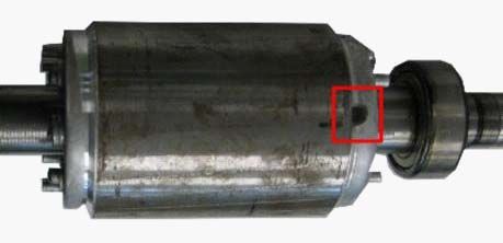
Sensors 2021, 21, 5076                                                                                          2 of 30

                         applied before it becomes a catastrophic one. Although the cage fault is a slowly developing
                         one, it is important to deploy fast and simple diagnostic techniques that can be applied
                         on-site, without the need for transmitting a huge amount of machine data to higher-level
                         processing centres, so saving valuable communications bandwidth resources. This requires
                         fast and simple fault diagnostic techniques, which can be implemented in embedded field
                         devices, such as digital signal processors (DSPs) or field-programmable arrays (FPGAs) [8].
                         For example, a growing trend in the condition monitoring of induction motors is the use of
                         smart sensors, attached to the motor frame, such as the SIEMENS Simotics Connect 400 [9],
                         or the ABB Ability Smart Sensor [10], which performs the diagnostic procedure locally,
                         and transmits the diagnostic results to the Internet of Things (IoT). Other scenarios that
                         benefits from fast diagnostic techniques are companies dedicated to diagnosis responsible
                         for monitoring big sets of motors, which might need several analyses in the case of alarm,
                         needing a quick response of the motor state to avoid unnecessary stops [11].
                               Among the different fault diagnostic techniques that can be deployed in CBM systems,
                         the use of digital twins is attracting a rising interest: a digital model of the IM is built,
                         and the model outputs (currents and voltages) are compared with the quantities mea-
                         sured at the machine terminals. Divergences between the predicted and measured values,
                         as well as the increase with time of these differences, are clear indications of a possible
                         fault. Recent developments in this field propose to integrate discrete component prog-
                         nosis in model-based CBMs of hybrid systems, with a new event-triggering mechanisms
                         using degradation model selection [12]. This methodology enables even the prognosis of
                         intermittent faults in discrete components, as shown in [13]. Digital twins of an IM can
                         be built using different approaches. The finite elements method (FEM) provides highly
                         accurate IM models [14], but it demands huge computing resources in terms of speed
                         and processing power, especially when simulating non-symmetrical, faulty IMs. This
                         hampers its use in low-power embedded units. On the contrary, analytical models, based
                         on a circuital approximation, can be very fast, but they lack the precision of FEM models.
                         Nevertheless, from a diagnostic point of view, it suffices that the analytical models can
                         reproduce accurately the effects of the faults in the IM currents or voltages, and they can
                         do this at a much higher speed and lower cost that FEM models [15]. As [16] points out,
                         these analytical models allow finding the most important effects of cage asymmetry and
                         require only the basic motor parameters. Another diagnostic area in which IM models are
                         used is in the training of neural networks or expert systems for fault diagnosis, which need
                         thousands of tests performed under different working conditions with controlled degrees
                         of IM faults. In this area, again, the speed of analytical models can give them a decisive
                         edge over FEM .
                               One of the main difficulties in the development of circuital models of the IM is the
                         dependency of the mutual and self inductances of the windings, and their derivatives,
                         on the rotor position. This is a complex, non-linear function, which depends on the
                         windings configurations, and on their relative positions [15]. Besides, these configurations
                         may become asymmetrical in case of cage faults, rendering useless many labor-saving
                         procedures that can only be applied to symmetrical windings. Indeed, mutual and self
                         inductances of rotor and stator windings must be recalculated for each type of fault.
                         A common simplification is to consider only pure sinusoidal air-gap spatial waves, that
                         is, approximating the winding inductances by their fundamental harmonic component.
                         Nevertheless, the complex interactions between spatial and time harmonics that generate
                         the characteristic fault harmonics in the machine current cannot be accurately reproduced
                         by these simplified models, what prevents their use for fault simulation and diagnosis
                         of SCIMs.
                               Diverse approaches have been presented in the technical literature for an accurate
                         computation of the inductance matrix needed in analytical models of the SCIM under fault
                         conditions. In [17,18], this matrix is obtained by direct measurements, in [19] a FEM model
                         has been used for inductance computation, and in [20,21] a hybrid FEM-analytical method
                         has been presented. In [22], a reduced-order model of the rotor cage is used to take into
Sensors 2021, 21, 5076 3 of 30
account non-sinusoidal magnetomotive (MMF) forces. Saturation and non-linearities of
the magnetic circuit have been taken into account in circuital IM models using modified air
gap length functions [23], the co-energy based method [15], or a complex multi-harmonic
model [24]. In [25], the partial-inductance method has been proposed for obtaining the
inductance matrix using an analytical solution of the air gap magnetic vector potential.
Linear models allow for a further simplification, using a one-dimensional analysis in
which the radial component of the flux density is determined as a function of the angular
position of the coils along the air gap circumference [15]. Many formulas for determining
the self and mutual inductances of an arbitrary pair of coils situated in the air gap zone
have been presented in the technical literature, as in [26,27], and they are the base of the
winding function approach (WFA) [23,28]. Nevertheless, this approach requires complex
winding functions that depend on the relative position of the coils, on the coils MMF
functions, on the permeance function of the air gap, and on the rotor position, leading to
triple integrals for each pair of coils [15]. On the contrary, the winding tensor function
approach [29] uses the conductor as the most basic unit, instead of the coil, and gives the
self and mutual inductances of the IM windings applying routine tensor algebra functions,
following Kron’s method [26,30].
The methodology proposed in this work greatly simplifies the process for calculating
the parameters of the SCIM model under different rotor asymmetry conditions, using a
novel approach: instead of obtaining directly the parameters of the SCIM under faulty
conditions, which is a difficult computation that must be done for each type of fault
or combination of faults, only the parameters of the healthy SCIM are obtained, using
the winding tensor approach [29]. The parameters of the SCIM under any type of rotor
asymmetry (bar breakages, end-ring breakages) are then obtained using simple connection
tensors, whose elements are only zeros, ones or minus ones, and applying routine tensor
algebra operations. It is proven, both theoretically and experimentally, that this simple
approach is able to account for any type and number of rotor asymmetry faults, so avoiding
a cumbersome setup of the equations of all the possible asymmetrical rotor circuits that
correspond to these faults.
The paper’s structure is the following one. In Section 2, the analytical model of the
SCIM is presented. In Section 3, the parameters of the SCIM are obtained in a primitive
reference frame, where they have its simplest expression. In Section 4, the model of a SCIM
in healthy state is developed using these parameters and a simple tensor transformation.
The model of the faulty SCIM is derived by and additional tensor transformation of the
healthy SCIM model in Section 5. An experimental validation of the proposed approach
is carried on in Section 6 using a commercial SCIM with different cage faults. Finally,
Section 7 presents the conclusions of this work.
2. Analytical Model of the SCIM
Let us consider a generic IM with ns stator windings and nr rotor windings, with a
total number of windings n = ns + nr . A holonomic reference frame [26] will be used in
this paper, with an electrical axis rigidly connected to each winding, as seen in Figure 1.
Therefore, the axes attached to the ns windings phases (s1 , s2 , . . . , sns , in Figure 1) will be
static, and those attached to the nr rotor windings (r1 , r2 , . . . , rnr , in Figure 1) will move
with the rotor.Sensors 2021, 21, 5076 4 of 30
s3 s2
r2 r1
s4 s1
r3 rnr
s5 sns
Figure 1. Coordinate system of the IM with an electrical axis rigidly connected to each phase, static
in the case of the ns stator windings and moving with the rotor in case of the nr rotor windings.
The n winding currents are the components of the current tensor i in this reference
frame, that is
s1 s2 ... sns r1 r2 ... r nr
t
(1)
i= i s1 i s2 ... i sns i r1 i r2 ... i r nr
where the superscript t stands for the transpose operator. For easy of notation, if the
axes information in (1) is omitted, then only the tensor components will be indicated as
i = [is1 , is2 , . . . , isns , ir1 , ir2 , . . . , irnr ]t .
The tensor equations of voltage and torque of the IM in this coordinate system
are [26,31]
dϕ
• Equation of voltage: e = Ri + dt
(2)
• Equation of torque: T= J dt − 12 it dL
dθ̇
dθ i
Besides the current tensor, i, the quantities that appear in (2) are the following ones:
• e is the voltage tensor. Its n components are the instantaneous terminal voltages
applied to each winding e = [es1 , es2 , . . . , esns , er1 , er2 , . . . , ernr ]t .
• ϕ is the flux linkage tensor. Its n components are the instantaneous flux linkages of
each winding ϕ = [ ϕs 1 , ϕs 2 , . . . , ϕs ns , ϕr 1 , ϕr 2 , . . . , ϕr nr ]t .
• R is the resistance tensor. It is a diagonal tensor, with n2 components, whose elements
are the resistances of the windings.
• L is the inductance tensor. It is a dyadic tensor, whose n2 components are the self and
mutual inductances of the windings. It relates the current and flux linkage tensors as
ϕ = L · i.
• The rest of the terms that appear in (2) are the instantaneous applied shaft torque T,
the rotor instantaneous angle θ and speed θ̇, and the moment of inertia of the rotor J.
The inductance tensor L can be expressed as the sum of two components, one with
the inductances corresponding to the main flux linkages, the main inductance matrix Lµ ,
and other with the leakage inductances Lσ , as
L = Lµ + Lσ (3)Sensors 2021, 21, 5076 5 of 30
End turns, end rings, and slots leakage inductances, included in the diagonal Lσ matrix,
need to be pre-calculated, as usual in the technical literature, where explicit expressions
for these inductances can be found in [32–34]. Only the analytical computation of Lµ in (3)
will be carried out in this work.
A Simulink model that implements (2) is shown in Figure 2. As seen in Figure 2,
the mutual inductances between the stator and rotor windings depend on the rotor position,
and must be updated at each step of the simulation.
k1 k1
MI MI
f1 f1
Matrix
Multiply 1 1
s s
Matrix
1 Multiply
s
1 1 2 3 J 2 3
Figure 2. Analytical model that implements (2) in Simulink.
The reference frame used for the analytical model of the IM in Figure 1 is not unique.
If the current tensor is expressed in a different reference frame, its new components i0
would be different than the old ones, i. Nevertheless, if the matrix C of the coordinate
transformation is given, then the relation between the old components and the new ones is
given by
i = C · i0 (4)
and the transformation law of the rest of tensors e, R and L is given, applying tensor
algebra, by
e0 = Ct · e
ϕ0 = Ct · ϕ
(5)
L0 = Ct · L · C
R0 = Ct · R · C
In the case that the new reference frame is also holonomic, with all the electrical axes
rigidly attached to the windings, then (2) remains valid, just substituting the old tensors by
the new ones [26], as
dϕ0
• Equation of voltage: e0 = R0 i 0 + dt
(6)
1 0t dL0 0
• Equation of torque: T = J ddtθ̇ − 2 i dθ i
In this work, only holonomic reference frames, with all the electrical axis rigidly
attached to the windings, will be used. Therefore, (6) will remain valid for all the reference
frames used for modelling the SCIM both in healthy and faulty conditions.
The parameters of the model of Figure 2, both in healthy and faulty conditions, are
obtained in this work using simple tensor transformations based on constructive data and
on the resistances and leakage inductances of stator windings, rotor bars and end-ring
segments. Most of these basic parameters can be found in the technical data provided by the
manufacturer of the IM, as in the case of the machine used for the experimental tests in thisSensors 2021, 21, 5076 6 of 30
work. If these specifications are not available, they can be estimated using offline [35–37] or
online parameter estimation techniques [38]. A comprehensive review of these techniques
can be found in [39]. Recently, artificial intelligence (AI) methods for parameter estimation
have been proposed in [40], or using differential evolution algorithms [41]. Additionally,
IM parameters change with temperature, frequency, and saturation, which has not been
considered in the model used in with work.
It is worth mentioning that the model of Figure 2 is a dynamical one. Therefore,
it can be applied to IMs working in stationary regime, or under transient conditions,
as in [42]. Besides, being an analytical model, it is very fast, and can be run in real time.
This opens the possibility of using it not only for fault diagnosis of IMs, which is the
focus of this work, but also for speed estimation in sensorless control systems [43], or for
reducing torque oscillations produced by space harmonics [44,45], among many other
technical applications.
3. Primitive Reference Frame of the SCIM
Let us consider an SCIM with ns stator windings and a cage with nb rotor bars. Instead
of deriving directly the inductance and resistance matrices of the rotor loops and stator
windings, a simpler reference frame will be used as starting point, the primitive reference
frame, as proposed in [26]. The matrices obtained in this simpler reference frame will be
converted to the final ones using easy tensor transformations.
Following the method of tensor analysis proposed by Kron in [26], the rotor cage
network is modelled first by considering bar and end ring currents as independent variables,
shown in Figure 3. The actual rotor cage parameters will be obtained from this primitive
network by using a transformation matrix that represents the connections between those
elements, and applying (5).
The characteristics of the primitive reference frame represented in Figure 3 are the
following ones:
• The stator electrical axes are attached to the ns stator windings (usually three for
industrial SCIMs). The unit vectors along these axes will be denoted as s1 , s2 , . . . , sns ,
and the components of the current tensor will be denoted as is1 , is2 , . . . , isns . All the
stator windings are considered to have the same resistance Rs and leakage induc-
tance Lσs .
• Each bar of the rotor cage has attached rigidly an electrical axis. The unit vectors along
these axes will be denoted as b1 , b2 , . . . , bnb , and the components of the current tensor
will be denoted as ib1 , ib2 , . . . , ibn . All the bars are considered to have equal resistance
b
Rb and leakage inductance Lσb .
• Each end ring segment of the cage has attached rigidly an electrical axis. The unit
vectors along the axes of the segments of one end ring will be denoted as f 1 , f 2 , . . . , f nb ,
and g1 , g2 , . . . , gnb for the opposite end ring. The components of the current tensor
along these axes will be denoted as i f1 , i f2 , . . . , i f n for the segments of one end ring
b
and i g1 , i g2 , . . . , i gnb for the opposite one. All the end ring segments are considered to
have equal resistance Re and leakage inductance Lσe .
Therefore, the primitive network of the SCIM is built by removing all interconnections
between the windings and short circuiting each, as shown in Figure 4.Sensors 2021, 21, 5076 7 of 30
Lσe Re if nb
if 1 if 2 if 3 if nb1
Lσe Re Lσe Re Lσe Re Lσe Re
Lσb Lσb Lσb Lσb Lσb
ib1 ib2 ib3 ibnb−1 ibnb
Rb Rb Rb Rb Rb
Lσe Re Lσe Re Lσe Re Lσe Re
ig1 ig2 ig3 if ng1
Lσe Re ignb
Figure 3. Primitive reference frame used for the rotor cage, with nb bars. Each bar and each end
ring segment have a rigidly attached coordinate axis. The bar and end ring segment currents are the
components of the current tensor in this frame. The bars are coupled to each other and to the stator
currents through their mutual inductances (not shown in this circuit). On the contrary, the end ring
segments do not couple with the other windings through mutual inductances.
Ls1 bnb
Ls1 b1 Lsns bnb
Ls1 sns Lsns b1 Lb1 bnb
Lσs Rs Lσs Rs Lσb Rr Lσb Rr Lσe Re Lσe Re
es esn
1 s
s1 sns b1 bnb f1 gnb
Figure 4. Primitive reference frame of the SCIM, found by removing all interconnections between
the windings, and short circuiting each. The arrows show the mutual impedances between stator
windings and cage bars. The end ring segments do not couple with the other windings through
mutual impedances.
In the primitive reference frame of Figure 4, the current tensor i p has (ns + 3 · nb )
components:
s1 . . . sns b1 . . . bnb f 1 . . . f n b g1 . . . g n b
t (7)
i p = is1 . . . isns ib1 . . . ibn i f1 . . . i fn i g1 . . . i g n b
b b
In this primitive reference frame, the voltages of the stator windings are considered to
be independent variables, while the voltages applied to the rotor windings are zero. That
is, the voltage tensor is given by
s1 . . . sns b1 . . . bnb f 1 . . . f n b g1 . . . g n b
t (8)
e p = e1 . . . e n s 0 ... 0 0 ... 0 0 ... 0
3.1. Resistance Tensor of the SCIM in the Primitive Reference Frame
The resistance tensor in the primitive reference frame R p is a diagonal tensor, of size
(ns + 3 · nb ) × (ns + 3 · nb ), with the following components (from now on, the matrix
elements with a zero value will be left blank, for easy of presentation):Sensors 2021, 21, 5076 8 of 30
s1 . . . sns b1 . . . bnb f 1 . . . f nb g1 . . . gnb
s1 R s
.. ..
. .
sns Rs
b1 Rb
.. ..
. .
R p = bn b Rb (9)
f1 Re
.. ..
. .
f nb Re
g1 Re
.. ..
. .
gn b Re
3.2. Leakage Inductance Tensor of the SCIM in the Primitive Reference Frame
The leakage inductance tensor in this reference frame, L pσ (3), is also a diagonal tensor,
of size (ns + 3 · nb ) × (ns + 3 · nb ), with the following components:
s1 . . . sns b1 . . . bnb f 1 . . . f n b g1 . . . g n b
s1 Lσs
.. ..
. .
sns Lσs
b1 Lσb
.. ..
. .
L pσ = bnb Lσb (10)
f1 Lσe
.. ..
. .
f nb Lσe
g1 Lσe
.. ..
. .
gn b Lσe
It is worth mentioning that, in the primitive reference frame, the resistance (9) and the
leakage inductance (10) matrices are diagonal ones.
3.3. Main Inductance Tensor of the SCIM in the Primitive Reference Frame
The main inductance tensor in this reference frame, corresponding to the main flux
linkages, L pµ (3), is a dyadic tensor of size (ns + 3 · nb ) × (ns + 3 · nb ), with the follow-
ing components:Sensors 2021, 21, 5076 9 of 30
s1 ... sns b1 ... bn b f 1 . . . f n b g1 . . . g n b
s 1 L s1 s1 . . . L s1 s n s Ls1 b1 . . . L s 1 bn
b
.. .. ..
. . . ... ... ... ...
sns Lsns s1 . . . Lsns sns Lsns b1 · · · Lsns bn
b
b1 Lb1 s1 . . . Lb1 sns Lb1 b1 · · · Lb1 bn
b
.. .. ..
. . ... ... ... . ...
L pµ = bnb Lbn s . . . L bn s L bn b · · · L bn b (11)
b 1 b ns b 1 b nb
f1
..
.
f nb
g1
..
.
gn b
As displayed in L pµ (11), the mutual inductances between the end ring segments and
the rest of the windings due to the main flux linkages are zero, because their only flux
linkages are the leakage ones. As for the rest of the components of (11), they depend on
the actual stator and rotor winding configurations, and, besides, the mutual inductances
between stator and rotor windings also depend on the rotor angular position. Among the
many available methods in the technical literature for obtaining their values (FEM, WFA,
etc.), in this work the winding tensor approach has been selected, which is described briefly
in the next subsection.
3.4. Computation of the Main Inductances of the SCIM Using the Winding Tensor Approach
Neglecting the iron saturation and losses, mutual inductances depend only on the
geometry of the system [46]. Only the radial component of the main flux that crosses the
smooth air gap is considered in this work, and the iron permeability has been considered as
infinite. The analytical computation of mutual inductances considering also the tangential
component of the flux can be found in [25], and with non-uniform air-gap in [29]. A higher
precision can be achieved using numerical methods, such as those based in FEM [20,47],
but at the cost of an increased computing complexity. Nevertheless, the simple, analytical
approach followed in this work has proven to be able to reproduce correctly the fault
harmonics of the cage fault, while keeping a low computational burden.
A simplified computation of the self and mutual inductances between the IM windings
can be made assuming a sinusoidal distribution of their MMFs, thereby neglecting the
spatial harmonics generated by the windings distribution. This simplification hampers the
use of the analytical model presented in Figure 2 for fault diagnosis, because in case of a
fault there are complex interactions between spatial and time harmonics that can not be
reproduced by such a simplified model. In [26], the calculation of self and mutual winding
inductances with spatial harmonics was made by first establishing the mutual inductance
between two elementary coils, in different relative positions, and then transforming it into
winding inductances using a transformation matrix, as in (5). In [29], a similar procedure
was presented, but using a single conductor instead of a coil as the most basic unit, which
avoids the need to establish a different winding function for each relative position between
two coils.Sensors 2021, 21, 5076 10 of 30
For using the conductor as the most basic unit, a reference frame is established by
considering that the circular air gap is evenly divided into N segments, and that each of
them is filled with an elementary conductor, located in the air gap zone, with an electrical
axis attached to it (see Figure 5). In [25], two layers of conductors have been considered
instead, one placed on the inner stator surface and the other one placed on the outer rotor
surface. The maximum spatial harmonic of the winding that can be represented in this
reference frame is N/2, and, therefore, a high value of N is selected (N = 3600 in [29]).
2π
N
c4
c3
c2
c1
cN
cN −1
Figure 5. Reference frame constituted by N independent conductors placed in the air gap. The N
components of the air gap current tensor in this system, ic , are the currents through each elemen-
tary conductor.
In this reference frame, the air gap current tensor components, ic , are the currents
through each elementary conductor.
c1 c2 ... cN
t
(12)
ic = i c1 i c2 ... ic N
In the reference frame of Figure 5, the main inductance tensor, Lcµ , is a N × N dyadic
tensor, given by
c1 c2 ... cN
c1 L c1 c1 L c1 c2 . . . L c1 c N
Lcµ = c2 L c2 c1 L c2 c2 . . . L c2 c N (13)
.. .. .. ..
. . . . ...
c N L c N c1 L c N c2 . . . L c N c N
whose component (i, j), Lci c j , is the mutual partial inductance [25] between the conductors
placed at positions (i − 1) · 2π 2π
N and ( j − 1) · N , with i, j = 1, 2, . . . , N. In case of an IM with
uniform air gap length, as represented in Figure 5, and considering that the air gap is smallSensors 2021, 21, 5076 11 of 30
compared to its radius, Lci c j depends only on the angular separation between conductors i
and j, and is given by [42]
µ0 · l · r · π 1 | i − j | 2
Lcµ (i, j) = Lci c j = · − (14)
g 2 N
where µ0 = 4π10−7 , l is the effective length of the stator bore, r is the radius at the center
of the air gap, and g is the air gap length.
The expression of the mutual inductance between conductors Lcµ has also been
obtained considering an analytic two dimensional field analysis in [25,48], or a numerical
model in [47]. Besides, it has been obtained in the case of a non-uniform air gap due to
rotor eccentricity in [29,49].
From (14), the components of Lcµ are the same for every IM, except for the scaling
µ · l ·r · π
factor 0 g , which depends only on the geometrical dimensions of the machine l, r and g.
Besides, Lcµ is a circulant, symmetrical, matrix, where every column is obtained by shifting
one position the preceding column.
The relation between the old currents ic (12), and the new ones i p (7) can be formulated
using a ( N × (ns + 3nb )) winding tensor Cc as (4)
ic = Cc · i p (15)
where
s1 ... sns b1 ... bn b f 1 . . . f n b g1 . . . g n b
c1 z1s1 . . . z1sns z1b1 . . . z1bn 0 ... 0 0 ... 0
b
Cc = c2 z2s1 . . . z2sns z2b1 . . . z2bn 0 ... 0 0 ... 0 (16)
b
.. .. .. .. .. .. .. .. ..
. . ... . . ... . . ... . . ... .
c N z Ns1 . . . z Nsns z Nb1 . . . z Nbn 0 ... 0 0 ... 0
b
The winding tensor Cc (16) represents the connections between the conductors of each
winding. Its (i, j) element contains the number of conductors zij of winding j contained in
the angular interval 2π/N (Figure 5), centred at (i − 1) · 2π N , with the corresponding sign
according to the direction of the current. For example, the distribution of the conductors
along a stator slot that contains Zslot conductors of a given stator winding, and has a
slot opening equal to b, would be a constant value of zsc = Zslot /b · (2πrs )/N air gap
conductors per interval along the slot opening (with its corresponding sign), where rs is
the inner radius of the stator bore. In this way, the effects of the slot width or the rotor bar
inclination can be represented with up to N/2 spatial harmonics. In the case of the rotor
end rings, as they have no conductors in the air gap, the corresponding columns in Cc
(e1 , . . . , enb , f 1 , . . . , f nb ) are zero. These columns have been maintained in (16) for the sake
of completeness.
The main inductance tensor of the windings in the reference frame of Figure 3, L pµ (11),
can be obtained from the main inductance tensor of the conductors in the reference frame of
Figure 5, Lcµ (13), applying the routine tensor algebra transformation (4) with the winding
tensor Cc (16), as
L pµ = Cc t · Lcµ · Cc (17)
The winding tensor Cc (16) must be obtained for the N possible angular positions
of the rotor (θk = (k − 1) · 2π
N , with k = 1, . . . , N). Nevertheless, the columns of Cc
corresponding to the ns stator windings do not depend on the rotor position, and the
columns of Cc corresponding to the rotor windings for a given rotor position θk are the
same as the columns defined with the rotor at the origin (θ0 = 0), but circularly shifted
k positions.Sensors 2021, 21, 5076 12 of 30
In (16), no restrictions are imposed on the connections of the conductors of each
winding, which can be arbitrarily complex, as in the case of asymmetrical windings (turn-
to-turn short circuits, etc.). Nevertheless, in case of a healthy machine, the configuration of
all the stator and rotor windings are the same, respectively. Therefore, the column of Cc
corresponding to the kth stator winding (sk ) is equal to the column of the first stator winding
(s1 ), but circularly shifted k · N/ns positions. The same applies to the rotor windings, but in
this case the circular shift is k · N/nb positions. In this particular case, the computation
of (16) can be performed in a very fast way using the convolution theorem, based on the
the circulant properties of matrix Lcµ , as presented in [42].
4. Analytical Model of the SCIM in Healthy State
In Section 3, a primitive reference frame has been used, considering the bar and the
end ring segment currents as independent variables. The number of rotor equations of the
SCIM in this reference frame is very high, equal to the sum of the number of rotor bars and
twice the number of end-ring segments. To reduce it, rotor loop equations are established
in this section, taking into account the connections between the cage components (bars and
end ring segments), using a connection tensor. The parameters of the SCIM using rotor
loop currents will be found by applying routine tensor algebra (5).
4.1. Connection Tensor for the Rotor Bars and End Ring Segments
The new reference frame consists of attaching an electrical axis to each rotor loop,
which is constituted by two adjacent rotor bars and their connecting end ring segments,
as displayed in Figure 6.
Lσe Re
if
Lσe Re Lσe Re Lσe Re Lσe Re
Lσb Lσb Lσb Lσb Lσb
i l1 i l2 i l3 ilnb −1
Rb Rb Rb Rb Rb
Lσe Re Lσe Re Lσe Re Lσe Re
ig
Lσe Re
Figure 6. Rotor loops in a squirrel cage rotor of nb bars. There are nb − 1 rotor loops, formed by two
consecutive bars, coupled to each other and to the stator windings through their mutual inductances
(not displayed in this schema). Besides, there are two end ring loops, which do not couple with any
other windings through mutual inductances.
Therefore, in the reference frame of Figure 6, the current tensor i will have (ns + nb + 1)
components, the currents in the ns stator windings, the nb − 1 rotor loops and the two end
ring loops:
s1 ... sns l1 ... l n b −1 f g
(18)
i= i s1 ... i sns i l1 ... i ln ie ig t
b −1Sensors 2021, 21, 5076 13 of 30
The relation between the primitive network currents
i p (7), and the new ones i (18)
can be formulated using a (ns + 3nb ) × (ns + nb + 1) connection tensor C p , with the aid
of Kirchoff’s laws, as
i p = Cp · i (19)
The connection tensor C p can be established by direct comparison of Figure 3 and
Figure 6, just indicating the connections between the individual bars and end ring segments
forming each rotor loop as:
s1 . . . s n s l1 l2 . . . l n b −2 l n b −1 f g
s1 1
.. ..
. .
sns 1
b1 1
b2 −1 1
.. ..
. .
bn b − 2 −1 1
bn b − 1 −1 1
bn b −1
f1 1 −1
Cp = (20)
f2 1 −1
.. .. ..
. . .
f n b −2 1 −1
f n b −1 1 −1
f nb 1
g1 −1 1
g2 −1 1
.. .. ..
. . .
g n b −2 −1 1
g n b −1 −1 1
gn b −1
Using the connection tensor C p in (4), the tensors’ components in this new reference
frame are obtained directly from their components in the primitive reference frame as
voltage tensor =e C pt · ep
resistance tensor R = C pt · Rp · Cp
(21)
leakage inductance tensor Lσ = C pt · L pσ · Cp
main inductance tensor Lµ = C pt · L pµ · CpSensors 2021, 21, 5076 14 of 30
For example, the resistance tensor R (rotor loop resistances in Figure 6) is obtained,
applying (21), as
s1 . . . s n s l1 l2 ... l n b −2 l n b −1 f g
s1 R s
.. ..
. .
sns Rs
l1 Rbe − Rb − Re − Re
R= l2 − Rb Rbe − Rb − Re − Re (22)
.. .. .. .. .. ..
. . . . . .
l n b −2 − Rb Rbe − Rb − Re − Re
l n b −1 − Rb Rbe − Re − Re
f − Re − Re − Re − Re − Re nb · Re
g − Re − Re − Re − Re − Re nb · Re
which checks with the expression given in [29], with Rbe = 2( Rb + Re ). That is, the careful
derivation of the circuit equations of the network of Figure 6 has been replaced by routine
laws of tensor transformations applied to the much simpler primitive network parameters,
just the diagonal resistance matrix (9), using a transformation matrix whose elements are
ones, minus ones and zeros (20).
4.2. Connection Tensor for the Stator Windings
In the primitive reference frame of Section 3, the stator currents have been considered
as independent variables. In this section, the connections between the stator windings are
taken into account, using a connection tensor, and the actual parameters of the SCIM will
be found by applying routine tensor algebra (5). The stator currents can be considered
as independent variables if each winding is fed with an independent power source, or if
they are connected in star configuration, fed from a power line with a distributed neutral
connected to the neutral point of the star. In any other case, the connection tensor of the
stator windings must be applied to the primitive tensors to obtain the actual SCIM ones.
For example, in case of a star connection of the stator windings, fed from a power line
without distributed neutral, the following constraint of the stator currents applies:
ns n s −1
∑ i si = 0 =⇒ isns = − ∑ i si (23)
i =1 i =1
This constraint reduces the number of independent stator currents by one. Therefore,
the current tensor (18) will have (ns + nb ) components, the currents in the ns − 1 stator
windings, the nb − 1 rotor loops and the two end ring loops:
s1 ... s n s −1 l1 ... l n b −1 f g
(24)
i= i s1 ... i s n s −1 i l1 ... i ln ie ig t
b −1Sensors 2021, 21, 5076 15 of 30
and the connection tensor C p (20) becomes:
s1 . . . s n s −1 l1 l2 . . . l n b −2 l n b −1 f g
s1 1
.. ..
. .
s n s −1 1
s n s −1 −1 −1
b1 1
b2 −1 1
.. ..
. .
Cp = (25)
bn b − 1 −1 1
bn b −1
f1 1 −1
.. .. ..
. . .
f nb 1 −1
g1 −1 1
.. .. ..
. . .
gn b −1 1
For ease of presentation, in this work it will be assumed that the stator currents are
independent variables, and, therefore, the connection tensor (20) will be used for obtaining
the SCIM parameters, and the voltage tensor (8) will not be modified by the connection
tensor C p . That is, e = e p in (21).
4.3. Voltage and Torque Equations of the SCIM with a Healthy Rotor Cage
As seen in (21), the parameters of the SCIM with a healthy cage in the rotor loop frame,
Figure 6, can be obtained directly from the parameters of the SCIM in the primitive reference
frame, Figure 6, where they adopt their simplest form (diagonal matrices for the resistance
and leakage inductance tensors, partial inductances between single rotor bars and stator
windings). The new parameters have been found by routine tensor transformations, using
a simple connection matrix C p , whose element are ones, minus ones and zeros, which just
reflect the connections between bars and end ring segments in the healthy rotor cage (20).
As this transformation is holonomic (the new rotor axes remain rigidly attached to the rotor
windings), the voltage and torque equations (2), being a tensorial equation, remain valid,
just replacing the old by the new, transformed SCIM tensors.
5. Analytical Model of the SCIM with Rotor Cage Faults
In this section, the parameters of a SCIM with rotor cage faults is obtained from the
resistance and inductance tensors of the healthy machine, by defining a transformation
tensor that takes into account each type of fault, and applying routine tensor transformation
laws. Three cases will be considered next: a cage with a broken bar, a cage with two non-
consecutive rotor bars, and a cage with a broken end ring segment. Other faults such as
non-consecutive broken bars, or the combined breakage of end ring segments and rotor
bars can be treated in a similar way.
5.1. Analytical Model of the SCIM with a Broken Rotor Bar
The rotor network of an SCIM with a single broken rotor bar (b2 in this example) can
be established as depicted in Figure 7. This electrical network is derived from the healthySensors 2021, 21, 5076 16 of 30
rotor cage shown in Figure 6, but now the first rotor loop (which contains the broken bar
b2 ) is formed by two non-consecutive rotor bars (b1 and b3 ).
Lσe Re
i0f
Lσe Re Lσe Re Lσe Re Lσe Re
Lσb Lσb Lσb Lσb
i0l1 i0l2 i0lnb −2
Rb Rb Rb Rb
Lσe Re Lσe Re Lσe Re Lσe Re
i0g
Lσe Re
Figure 7. Rotor loops in a squirrel cage rotor of nb bars with a single broken bar (b2 ). It is similar to
the circuits in a healthy rotor cage shown in Figure 6, but now the first rotor loop is formed by two
non-consecutive bars (b1 and b3 ).
In the reference frame of Figure 7, the current tensor i0 will have (ns + nb ) components,
the currents in the ns stator windings, the nb − 2 rotor loops and the two end ring loops.
s10 ... s0ns l10 ... ln0 b −2 f0 g0
(26)
i0 = is0 1 ... is0 ns il0 ... il0n i0f i0g t
1 b −2
The transformation tensor that relates the currents in the healthy and in the faulty
reference frame, Cb2 , so that i = Cb2 · i0 , can be established by direct comparison of
Figures 3 and 7, as:
s10 . . . s0ns l10 l20 . . . ln0 b −3 ln0 b −2 f 0 g0
s1 1
.. ..
. .
sns 1
l1 1
l2 1
Cb2 = (27)
l3 1
.. ..
. .
l n b −2 1
l n b −1 1
f 1
g 1
That is, what Cb2 reflects is simply that the effect of a broken bar in Figure 7 can be
represented by equating the currents in the two rotor loops that contain the missing bar,
in this case loops l1 and l2 . As the transformation tensors of the current form a group, theirSensors 2021, 21, 5076 17 of 30
combined effect is obtained by a simple product. Therefore, the final tensors of the SCIM
with a broken bar of Figure 7 are obtained, using both connecting tensors C p and Cb2 as
resistance tensor R0 = (C p · Cb2 )t · Rp · (C p · Cb2 )
leakage inductance tensor L0σ = (C p · Cb2 )t · L pσ · (C p · Cb2 ) (28)
main inductance tensor L0µ = (C p · Cb2 )t · L pµ · (C p · Cb2 )
5.2. Analytical Model of the SCIM with Two Non-Consecutive Broken Rotor Bars
The electrical rotor network of a SCIM with two non-consecutive broken rotor bars (b2
and b4 in this example) can be established as depicted in Figure 8. This network is similar
to the healthy rotor cage shown in Figure 6, but now the first two rotor loops contain the
non consecutive broken bars.
Lσe Re
i0f
Lσe Re Lσe Re Lσe Re Lσe Re
Lσb Lσb Lσb Lσb
i0l1 i0l2 i0lnb −2
Rb Rb Rb Rb
Lσe Re Lσe Re Lσe Re Lσe Re
i0g
Lσe Re
Figure 8. Rotor loops in a squirrel cage rotor of nb bars with two non-consecutive broken bars (b2
and b4 ). It is similar to the circuits in a healthy rotor cage shown in Figure 6, but now the the first two
rotor loops contain non-consecutive broken bars.
In the reference frame of Figure 8, the current tensor i0 will have (ns + nb − 1) compo-
nents, the ns stator currents, the nb − 3 rotor loop currents and the two end ring currents.
s10 ... s0ns l10 ... ln0 b −3 f0 g0
(29)
i0 = is0 1 ... is0 ns il0 ... il0n i0f i0g t
1 b −3
The transformation tensor that relates the currents in the healthy (18) and in the faulty
(29) reference frames, Cb2 b4 , so that i = Cb2 b4 · i0 , can be established by direct comparison
of Figures 3 and 7, as:Sensors 2021, 21, 5076 18 of 30
s10 . . . s0ns l10 l20 . . . ln0 ln0 b −3 f 0 g0
b −4
s1 1
.. ..
. .
sns 1
l1 1
l2 1
Cb2 b4 = l3 1 (30)
l4 1
.. ..
. .
l n b −2 1
l n b −1 1
f 1
g 1
That is, what Cb2 b4 reflects is simply that the effect of two broken bars in Figure 8
can be represented by making equal the currents in the two rotor loops that contain each
missing bar. As the transformation tensors of the current form a group, their combined
effect is obtained by a simple product. Therefore, the final tensors of the SCIM with two
non-consecutive broken bars of Figure 8 are obtained, using both connecting tensors C p
and Cb2 b4 as
resistance tensor R0 = (C p · Cb2 b4 )t · Rp · (C p · Cb2 b4 )
leakage inductance tensor L0σ = (C p · Cb2 b4 )t · L pσ · (C p · Cb2 b4 ) (31)
main inductance tensor L0µ = (C p · Cb2 b4 )t · L pµ · (C p · Cb2 b4 )
5.3. Analytical Model of the SCIM with a Broken End Ring Segment
The rotor network of a SCIM with a broken end ring segment ( f 1 in this example)
can be established as depicted in Figure 9. This circuit is similar to the circuit of a healthy
rotor cage shown in Figure 6, but now the first rotor loop (which contains the broken end
segment ) includes the whole end ring loop.
Lσe Re
Lσe Re Lσe Re Lσe Re
Lσb Lσb Lσb Lσb Lσb
i0l1 i0l2 i0l3 i0lnb −1
Rb Rb Rb Rb Rb
Lσe Re Lσe Re Lσe Re Lσe Re
i0g
Lσe Re
Figure 9. Rotor loops in a squirrel cage rotor of nb bars with a single broken end ring segment () f 1 ).
It is similar to the circuits in a healthy rotor cage shown in Figure 6, but now the first rotor loop
includes the whole end ring loop.Sensors 2021, 21, 5076 19 of 30
In the reference frame of Figure 9, the current tensor i0 will have (ns + nb ) components,
the ns stator currents, the nb − 1 rotor loop currents and the healthy end ring current.
s10 ... s0ns l10 ... ln0 b −2 ln0 g0
b −1
(32)
i0 = is0 1 ... is0 ns il0 ... il0n ie0 i0g t
1 b −2
The transformation tensor that relates the currents in the healthy (18) and in the faulty
(32) reference frames, C f1 , so that i = C f1 · i0 , can be established by direct comparison of
Figures 3 and 9, as:
s10 . . . s0ns l10 l20 . . . ln0 b −3 ln0 b −2 ln0 g0
b −1
s1 1
.. ..
. .
sns 1
l1 1
l2 1
C f1 = (33)
l3 1
.. ..
. .
ln0 b −2 1
ln0 −1 1
b
f 1
g 1
That is, what C f1 reflects is simply that the effect of a broken end ring segment in
Figure 9 can be represented by making equal the current in the rotor loop that contain
the missing end ring segment f 1 , in this case loop l1 , and the current in the end ring loop.
As the transformation tensors of the current form a group, their combined effect is obtained
by a simple product. Therefore, the final tensors of the SCIM with a broken end ring
segment of Figure 9 are obtained, using both connecting tensors C p and C f1 as
resistance tensor R0 = (C p · C f1 )t · Rp · (C p · C f1 )
leakage inductance tensor L0σ = (C p · C f1 )t · L pσ · (C p · C f1 ) (34)
main inductance tensor L0µ = (C p · C f1 )t · L pµ · (C p · C f1 )
5.4. Voltage and Torque Equations of the SCIM with Cage Faults
As commented in Section 4.3, the parameters of the SCIM with a faulty cage can be
obtained directly from the parameters of the SCIM in the primitive reference frame (the
simplest one) by routine tensor transformations. Simple connection matrices C p (20), Cb2 (27),
Cb2 b3 (30), and C f1 (33), whose elements are ones and zeros, which reflect the connections
between bars and end ring segments in the faulty rotor cage, are used in this transformations.
As the new rotor axes remain rigidly attached to the rotor windings, the voltage and torque
Equations (2) remain valid, just using the transformed SCIM tensors. That is
0 0 0
R0 i0 + L0 di 0 dL
e
= dt + i dθ θ̇
0 (35)
T = J ddtθ̇ − 12 i0t dL
dθ i
0
where e0 = e, because the stator windings voltages have not been changed (only rotor cage
faults have been considered).Sensors 2021, 21, 5076 20 of 30
5.5. Analytical Model of the SCIM with Rotor Faults in Progress
In some cases, the faulty rotor bar or end ring segment are not completely broken,
but their resistance or leakage reactance are different from normal values due to a fault
in progress, such as an oxidation process [50]. In this case, the parameters of the faulty
rotor part are simply adjusted in the corresponding diagonal element of the primitive
resistance (9) or leakage inductance tensor (10). In this way, the proposed model can be
applied to the prognosis of incipient broken rotor bars in an induction motor, as in [51],
or half broken bars, as in [52]. Nevertheless, as [51] states, the deterioration of the bar is
a highly non-linear process, and more advanced physical models, such as multi-physics
finite-element analysis and fatigue testing would be necessary to establish a non-linear
failure model for the prognosis of incipient broken bar faults.
6. Experimental Validation
The validation of the proposed approach has been carried out by the simulation and
experimental tests of a commercial squirrel-cage induction motor, whose characteristics are
given in Appendix A. The types of faults that have been used for the experimental valida-
tion of the proposed model are broken bars faults: a single broken bar, two consecutive
broken bars, and two non-consecutive broken bars. In fact, major motor manufacturers
have reported cases where the damaged bars appear randomly distributed around the
rotor perimeter, indicating that the failure of non-adjacent bars is fairly common in large
cage induction motors.
6.1. Experimental Setup
The test equipment, displayed in Figure 10, consists of a current clamp, whose charac-
teristics are given in Appendix B, a 200 pulse/revolution incremental encoder, a Yokogawa
DL750 oscilloscope and a personal computer (Appendix C) connected to it via an intranet
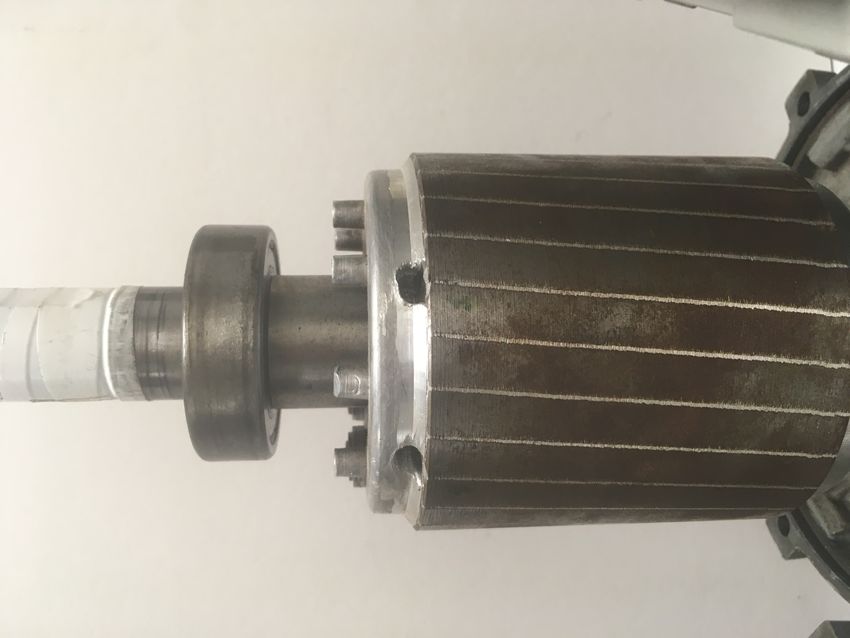
network. The broken bar fault has been artificially produced by drilling a hole in the
selected bars, as shown in Figure 10.
Figure 10. Experimental setup: measurement equipment (left), and rotor of the motor whose
characteristics are given in Appendix A, with a broken bar (right).
The rotor cage faults are detected using the motor current signature analysis (MCSA)
method. It is based on the identification in the current spectrum of the characteristic fault
harmonic components generated by the fault, at frequencies given by
f bb = (1 + 2ks) f 1 k = ±1, ±2, ±3 . . . (36)
where s is the motor slip, f 1 is the supply frequency, and k is the harmonic number.
For the tested and simulated motors, the rotor speed is the rated one, 1410 r.p.m, and the
supply frequency is f 1 = 50 Hz. The main fault harmonics used for the diagnosis are
those corresponding to a value k = ±1 in (36): the lower side-band harmonic (LSH),
with a frequency f LSH = (1 − 2s) f 1 , and the upper side-band harmonic (USH), with a
frequency f USH = (1 + 2s) f 1 . In case of the tested and simulated motors s = 0.06; therefore,
f LSH = (1 − 2 × 0.06) × 50 = 44 Hz, and f USH = (1 + 2 × 0.06) × 50 = 56 Hz.Sensors 2021, 21, 5076 21 of 30
In the case of a double bar breakage, the LSH magnitude is a function of the relative
position of the two broken bars. In [53], it has been shown that the ratio between the LSH
in case of double and single breakages depends on the angle between the broken bars as
LSHdouble
LSH pu = = |2 cos( pαbb )| (37)
LSHsingle
where p is the number of pole pairs and αbb is the angle between the two broken bars.
From (37), it can be deduced that if αbb approximates π/2p, that is, half a pole pitch, then
the second breakage reduces the magnitude of the LSH to a value lower than in the case of a
single breakage. Therefore, in this case a motor with two broken bars could be erroneously
diagnosed as a healthy motor. This behaviour is more challenging to simulate than the
single broken bar fault, and it has been selected to verify the validity of the proposed
model for fault diagnosis. Its experimental validation has been carried out using a set of
artificially damaged rotors with the three following faults: one broken bar, two consecutive
broken bars, and two non-consecutive broken bars, separated half a pole pitch, as seen
in Figure 11. An additional healthy rotor, with no broken bars, has been also used for
comparison purposes.
Figure 11. Tested rotors with faulty cages: one broken bar (left), two consecutive broken bars (centre)
and two non-consecutive broken bars (right).
The same stator has been used to perform all the experimental tests, to better control
the test conditions in all cases, as seen in Figure 12, right. The induction motor under test
(Appendix A) is connected via a belt coupling to a DC generator, which feeds a resistive
load, depicted in Figure 12. Both the resistive load and the field excitation of the generator
can be controlled, so that the induction machine works at rated speed 1410 r/min (s = 0.06).
The current of a stator winding has been measured using a sampling frequency of 5000 Hz,
during an acquisition time of 50 s.
Belt Coupling DC Generator
3 ∼ 400 V 50 Hz 220 V
Field Control
+
Load
Belt
Common Stator
- Different Faulty Rotors
Faulty Induction Motor DC Generator
Figure 12. Schema of the loading of the experimental machine (left) and experimental setup (right).
The induction motor under test (Appendix A) is connected to a DC generator via a belt coupling.
The DC machine feeds a resistive load. Both the resistive load and the field excitation can be controlled
so that the induction machine works at rated speed.Sensors 2021, 21, 5076 22 of 30
6.2. Analytic Model of the Tested Motor in Healthy Condition
In this section, the characteristic tensors of the tested SCIM (resistance, leakage induc-
tance and main inductance tensors) are obtained for the tested SCIM of Appendix A using
the proposed approach.
First, the main inductance tensor in the conductors reference frame of Figure 5, Lcµ (13)
is built by dividing the air gap circumference of the tested motor into a high number of
intervals, N = 1008, and applying (14). This value of N has been chosen to be a multiple of
the number of stator and rotor slots, to avoid numerical errors. The main inductance be-
tween two conductors located in the air gap has been represented in Figure 13 as a function
of their angular separation, which represents actually the first column of tensor Lcµ .
10-6
2.5
2
1.5
1
0.5
0
/2 3 /2 2
Figure 13. Main inductance between two conductors of the simulated machine, located in the air gap,
as a function of their angular separation.
The main inductance tensor, with the mutual inductances between stator windings
and rotor bars, is obtained by transforming the tensor Lcµ into the primitive reference
frame of Figure 3. This transformation (17) is made using the winding tensor Cc (16),
which contains the distribution of the conductors of the stator windings and the rotor bars,
for each rotor position, as the one shown in Figure 14.
10
5
0
-5
-10
/2 3 /2 2
0.03
0.02
0.01
0
/2 3 /2 2
Figure 14. Conductors per air gap interval of a stator winding (top) and a rotor bar (bottom).
The winding tensor Cc has been built using the distributions shown in Figure 14,
with the appropriate rotation of their elements for each winding and for each rotor position.
The main inductance tensor in the primitive reference frame has been obtained in this step
by applying the transformation Cc to Lcµ (17). Figure 15, top, presents the main inductanceSensors 2021, 21, 5076 23 of 30
between a stator winding and a rotor bar in the primitive reference frame of Figure 3,
and Figure 15, bottom, presents its angular derivative, as a function of the rotor position.
×10−4
2
1
0
−1
−2
/2 3 /2 2
×10−4
4
2
0
−2
−4
/2 3 /2 2
Figure 15. Mutual inductance between a stator winding and rotor bar of the tested machine as a
function of the rotor position (top), and its angular derivative (bottom).
Applying the connection tensor (25) to the tensors of the primitive reference frame
in (21), the machine tensors in the reference frame of Figure 6 are finally obtained for the
healthy SCIM. Figure 16, top, presents the main inductance between a stator winding and
a rotor loop in the reference frame of Figure 6, and Figure 16, bottom, presents its angular
derivative, as a function of the rotor position.
×10−5
5
0
−5
/2 3 /2 2
×10−4
2
0
−2
/2 3 /2 2
Figure 16. Mutual inductance between a stator winding and a rotor loop of the tested machine as a
function of the rotor position (top), and its angular derivative (bottom).
Once obtained the parameters of the tested SCIM in healthy condition, a transforma-
tion tensor is used to obtain its parameters under faulty condition. This tensor is differentSensors 2021, 21, 5076 24 of 30
for each type of fault, but it contains only zeros and ones to mark the type and position of
the considered cage fault. Its value for the cases of a single broken bar Cb2 has been given
in (27). The tensors for the cases of two consecutive broken bars Cb2 b3 and for the case of
two non-consecutive broken bars Cb2 b6 are given by:
s10 . . . s0ns l10 l20 . . . ln0 ln0 b −3 f 0 g0
b −4
s1 1
.. ..
. .
sns 1
l1 1
l2 1
Cb2 b3 = l3 1 (38)
l4 1
.. ..
. .
l n b −2 1
l n b −1 1
f 1
g 1
s10 . . . s0ns l10 l20 l30 l40 l50 . . . ln0 ln0 b −3 f 0 g0
b −4
s1 1
.. ..
. .
sns 1
l1 1
l2 1
l3 1
l4 1
Cb2 b6 = (39)
l5 1
l6 1
l7 1
.. ..
. .
l n b −2 1
l n b −1 1
f 1
g 1
6.3. Comparison between Experimental Tests and Simulations Using the Analytical Model of
the SCIM
The four tested motors have been simulated using the proposed approach, with the
model depicted in Figure 2. The spectrum of one of the simulated stator currents is shown in
Figure 17, where the main fault harmonics have been marked with text arrows, indicating
their magnitude. As predicted by (37), the LSH magnitude increases from the case of a single
broken bar, −37.93 dB, Figure 17b, to the case of two consecutive broken bars (broken bars
b2 , b3 ), −34.59 dB, Figure 17c. On the contrary, when the separation between the two broken
bars approaches half of a pole pitch (broken bars b2 , b6 ), the magnitude of the LSH decreases,
−45.68 dB, Figure 17d, which may be misdiagnosed as a healthy motor condition.You can also read