Uniform-momentum zones in a turbulent boundary layer subjected to freestream turbulence
←
→
Page content transcription
If your browser does not render page correctly, please read the page content below
Downloaded from https://www.cambridge.org/core. IP address: 46.4.80.155, on 11 Jul 2021 at 11:15:43, subject to the Cambridge Core terms of use, available at https://www.cambridge.org/core/terms. https://doi.org/10.1017/jfm.2021.102
J. Fluid Mech. (2021), vol. 915, A109, doi:10.1017/jfm.2021.102
Uniform-momentum zones in a turbulent
boundary layer subjected to freestream
turbulence
R. Jason Hearst1, †, Charitha M. de Silva2 , Eda Dogan3 and
Bharathram Ganapathisubramani3
1 Department of Energy and Process Engineering, Norwegian University of Science and Technology,
Trondheim NO-7491, Norway
2 School of Mechanical and Manufacturing Engineering, University of New South Wales,
Sydney 2052, Australia
3 Aerodynamics and Flight Mechanics Research Group, University of Southampton,
Southampton SO17 1BJ, United Kingdom
(Received 25 May 2020; revised 19 December 2020; accepted 26 January 2021)
The instantaneous structure of a turbulent boundary layer that has developed beneath
freestream turbulence (FST) was investigated with planar particle image velocimetry.
Measurements were performed in the streamwise–wall-normal plane at a position Rex =
U∞ x/ν = 2.3 × 10⁶ downstream of the boundary layer origin. FST was generated with
an active grid placed upstream of a boundary layer plate. Three cases were investigated
with FST intensity increasing from approximately zero to 12.8 %. It is shown that internal
interfaces, separating areas of approximately uniform momentum, are present for all
cases and show a dependence on the FST. In particular, the number and length of the
uniform-momentum zones (UMZs) decrease with increasing FST. The modal velocities
associated with the UMZs are distributed in approximately the same way regardless of
the condition of the outer flow, suggesting a degree of resilience of the instantaneous
structure to the freestream. Tracking the top edge of the upper-most UMZ revealed that
this contour approaches the wall for increasing FST. Finally, it is demonstrated that the
observed first-order phenomena in a turbulent boundary layer subjected to FST can be
modelled by superimposing an isotropic turbulence field on a turbulent boundary layer
field, which supports the hypothesis that the underlying structure of the boundary layer
appears to remain largely intact if the naturally occurring fluctuations in the turbulent
boundary layer exceed the energy of the FST.
Key words: homogeneous turbulence, turbulent boundary layers, boundary layer structure
† Email address for correspondence: jason.hearst@ntnu.no
© The Author(s), 2021. Published by Cambridge University Press. This is an Open Access article,
distributed under the terms of the Creative Commons Attribution licence (http://creativecommons.org/
licenses/by/4.0/), which permits unrestricted re-use, distribution, and reproduction in any medium,
provided the original work is properly cited. 915 A109-1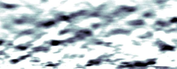
Downloaded from https://www.cambridge.org/core. IP address: 46.4.80.155, on 11 Jul 2021 at 11:15:43, subject to the Cambridge Core terms of use, available at https://www.cambridge.org/core/terms. https://doi.org/10.1017/jfm.2021.102
R. J. Hearst and others
1. Introduction
Identifying the flow structure that dominates the evolution of a turbulent boundary layer is
a topic of intense historical and contemporary research. The perspective held by a number
of researchers is that the boundary layer is instantaneously populated by a set of coherent
motions that dominate the distribution of Reynolds shear stress and transport in a turbulent
boundary layer (TBL) (Theodorsen 1952; Head & Bandyopadhyay 1981; Zhou et al. 1999;
Adrian, Meinhart & Tomkins 2000; Ganapathisubramani, Longmire & Marusic 2003;
Dong et al. 2017; Baidya et al. 2019). These motions have been shown to extend for
several boundary layer turnovers and ‘meander’ in the spanwise direction (Hutchins &
Marusic 2007). In a streamwise–wall-normal plane, these structures manifest as regions
of approximately uniform momentum typically referred to as uniform momentum zones
(UMZs) (Meinhart & Adrian 1995; Adrian et al. 2000; de Silva, Hutchins & Marusic
2016; de Silva et al. 2017; Laskari et al. 2018). These zones are believed to represent
the velocity entrained beneath a packet of hairpin vortices and are separated by sharp
shear events that create a layered instantaneous structure in a TBL (Eisma et al. 2015;
de Silva et al. 2017). Recent works have examined the time evolution of these structures
(Laskari et al. 2018), and their characteristics as a function of friction velocity Reynolds
number Reτ = Uτ δ/ν (de Silva et al. 2016), where Uτ is the friction velocity, δ is the
boundary layer thickness and ν is the kinematic viscosity. These instantaneous flow
features were also observed through reduced-order models of the large-scale coherence
in TBLs based on the Navier–Stokes equations (Saxton-Fox & McKeon 2017; McKeon
2019). Furthermore, UMZs have been used in models that are able to reproduce boundary
layer statistics up to fourth order (Bautista et al. 2019).
The general flow structure of UMZs located immediately above a wall with a bulk of
fluid moving above them is not limited to zero-pressure-gradient TBLs. UMZs have been
reported above the walls for turbulent channel (Kwon et al. 2014; Anderson & Salesky
2021) and pipe flows (Chen, Chung & Wan 2020; Gul, Elsinga & Westerweel 2020), both
of which have a ‘core’ region that is also turbulent. However, the existence of UMZs
has not been rigorously assessed for a TBL subjected to freestream turbulence (FST).
This flow is perhaps of more practical interest than the canonical zero-pressure-gradient
TBL because most engineering flows experience some degree of FST. Moreover, Hearst,
Dogan & Ganapathisubramani (2018) have shown that one can achieve Reynolds numbers
up to Reτ ≈ 5400 in a laboratory-scale (4 m long) wind tunnel by generating high
intensity FST above a TBL; such Reτ are typically only achievable in specialised facilities,
e.g. Nickels et al. (2005, 2007), Klewicki (2010) and Vincenti et al. (2013). These
flows also exhibit qualitatively similar spectrograms (Sharp, Neuscamman & Warhaft
2009; Dogan, Hanson & Ganapathisubramani 2016; Hearst et al. 2018), amplitude
modulation (Dogan, Hearst & Ganapathisubramani 2017) and spatial coherence (Dogan
et al. 2019) to canonical TBLs at similar Reτ ; thus, they may be a useful way for
fluid mechanics experimentalist to simulate high Reτ conditions in a typical size
facility.
Given the aforementioned similarities between a TBL subjected to FST and a
canonical TBL, one might expect to see similar instantaneous structures. To date,
the only instantaneous images available for these flows are the flow visualisations of
Hancock & Bradshaw (1989) and instantaneous fields extracted from the direct numerical
simulations (DNS) of You & Zaki (2019), Wu, Wallace & Hickey (2019) and Kozul
et al. (2020); while Dogan et al. (2019) had instantaneous flow fields, their work
focussed on the spatial statistics. The visualisations of Hancock & Bradshaw (1989)
appear to show a more jagged interface with the freestream for the turbulent case
915 A109-2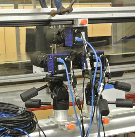
Downloaded from https://www.cambridge.org/core. IP address: 46.4.80.155, on 11 Jul 2021 at 11:15:43, subject to the Cambridge Core terms of use, available at https://www.cambridge.org/core/terms. https://doi.org/10.1017/jfm.2021.102
UMZs in a boundary layer subjected to FST
compared to the approximately laminar freestream. However, these images did not allow
for analysis of the internal boundary layer structure, nor were they quantitative. Kozul
et al. (2020) explicitly compared their instantaneous structure to that of Hancock &
Bradshaw (1989) and found qualitatively good agreement, however, the main focus
of their study was the statistics of the temporal boundary layer subject to a sudden
injection of FST. The DNS studies of You & Zaki (2019) and Wu et al. (2019)
roughly echo these results, however, they investigate only a single FST case at limited
Reynolds numbers. This is understandable as it is computationally expensive to compare
multiple cases and achieve higher Reynolds numbers. Moreover, there was no particular
focus on UMZs, although Wu et al. (2019) did identify an instantaneous ‘boundary
layer turbulence and freestream turbulence interface’ separating the two flow regions
for their one case. There is thus a need to perform detailed quantitative analysis
on the instantaneous structure within these TBLs subjected to different levels of
FST.
While investigating wall-bounded UMZs, de Silva et al. (2016) found that it was
important to exclude the velocity field above the instantaneous separation between the
wall-bounded flow and the approximately laminar freestream. This was done to improve
the detectability of UMZs present at the edge of the boundary layer, which would
otherwise be masked by the freestream velocity distribution. The primary reason for this is
that the freestream itself presents as a large UMZ when using the histogram modal velocity
process that has become common for this type of analysis, cf. Meinhart & Adrian (1995),
de Silva et al. (2016) and Appendix A. In fact, this idea is exploited by those studying the
‘quiescent core’ of turbulent channel flow to identify the edges of the core because it is
itself a UMZ (Kwon et al. 2014; Yang, Hwang & Sung 2016; Jie et al. 2019).
Given the existing body of work, an open question is how does the instantaneous flow
near a wall manifest beneath FST. We know that a canonical TBL has UMZs, and that their
number is Reτ dependent (de Silva et al. 2016). UMZs also exist in internal flows, which
feature a quiescent, but turbulent, core that is separate from the flow structure immediately
adjacent to the walls (Kwon et al. 2014; Yang et al. 2016; Jie et al. 2019; Chen et al. 2020;
Gul et al. 2020). Moreover, the TBL experiments of Laskari et al. (2018) detected UMZs
beneath a freestream of approximately 3 % turbulence. Finally, the recent study of Wu
et al. (2019) also identified an instantaneous separation between the freestream and the
wall-bounded flow in DNS of a zero-pressure-gradient TBL. Thus, UMZs exist in flows
with turbulence in the freestream, and the flow may be separated into the flow directly
influenced by the wall and the turbulent flow in the freestream or core. This has symmetries
with the mean velocity profiles of the various wall-bounded flows (zero-pressure-gradient
TBLs, internal flows, TBLs subject to FST), which share similar viscous sub-layers, buffer
layers and log regions, and primarily differ in the wake region. For the flows with some
degree of turbulence in the freestream or core, there is still an instantaneous separation
between the UMZs next to the wall and the freestream/core, and this is the top edge of
the upper-most UMZ. The problem which remains unaddressed is how the level of FST
influences the structure of the UMZs and the height to which they exist. This problem
cannot be addressed by internal flows whose centreline conditions are set by the inlet and
boundary conditions.
Accordingly, the present study seeks to examine the instantaneous structure of a
TBL over a flat plate subjected to FST in the streamwise–wall-normal plane using
planar particle image velocimetry (PIV). In particular, a canonical TBL is compared to
two flows with increasing FST intensity (u∞ /U∞ ). Section 2 details the experimental
set-up. Section 3 details the flow characteristics and identifies the mean differences
915 A109-3
Downloaded from https://www.cambridge.org/core. IP address: 46.4.80.155, on 11 Jul 2021 at 11:15:43, subject to the Cambridge Core terms of use, available at https://www.cambridge.org/core/terms. https://doi.org/10.1017/jfm.2021.102
R. J. Hearst and others
between the produced flows. Section 4 describes the detection methodologies for UMZs.
Section 5 investigates the existence of a zonal structure (composed of UMZs and
shear layers) in all three flows and comments on their differences. Section 6 discusses
the top edge of the upper-most UMZ. Section 7 examines if a simple model where
isotropic turbulence is superimposed on a canonical TBL can replicate some of the
phenomena observed in a TBL with FST. Finally, § 8 provides a summary of our
findings.
2. Experimental procedure
The physical design of the present experiments is the same as that of Dogan et al.
(2019). As such, the experiments are only briefly reviewed here and we refer the reader
to the aforementioned work for greater detail. All measurements were performed in the
0.9 m × 0.6 m × 4.5 m suction wind tunnel at the University of Southampton. The
freestream turbulence was generated by an active grid inspired by the original design of
Makita (1991). This apparatus features a series of square wings mounted to rotating round
rods that are actuated by stepper motors. By changing the grid parameters (e.g. speed of
rotation, incoming flow velocity, wing blockage) a certain degree of control authority can
be exerted over the turbulence intensity, anisotropy and length scales (Hearst & Lavoie
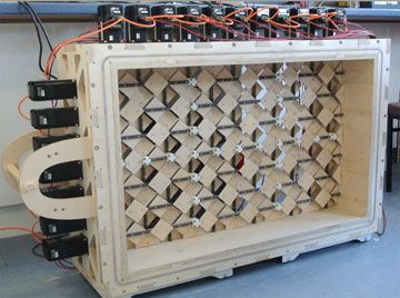
2015; Hearst & Ganapathisubramani 2017). The present grid is made up of a 11 × 7 array
of square wings mounted to the round rods. The spacing between grid rods is M = 81 mm,
and the wings themselves are 55.9 mm × 55.9 mm. A picture of the grid outside of
the wind tunnel is presented in figure 1(a). The boundary layer was formed on a flat
plate suspended above the wind tunnel floor. The flat plate began 300 mm downstream
of the grid and extended 4.1 m downstream. The boundary layer was tripped by a zig–zag
wire placed 90 mm from the leading edge of the flat plate. A schematic of the set-up along
with the reference coordinate system is provided in figure 1(b).
In the present study, three different cases are investigated: (i) a low turbulence intensity
case to represent a canonical TBL (REF), (ii) a moderate turbulence intensity case (FST-8)
and (iii) a high turbulence intensity case (FST-13). FST-8 and FST-13 are equivalent to
cases ‘B’ and ‘D’, respectively, from Dogan et al. (2016, 2017, 2019). For the two FST
cases, the active grid wing rotational rate is randomly varied between 2 and 6 Hz (modelled
after ‘case 14’ from Larssen & Devenport 2011), and the operational parameters for the two
cases differ only in that they use wings with different blockage. FST-8 employed square
wings with holes, while FST-13 employed solid square wings. The square wings with holes
have approximately 75 % of the surface area of the solid square wings. Using the same
rotational parameters but changing the wing geometry results in FST with similar length
scales and isotropy, but different turbulence intensity (Hearst & Lavoie 2015). All three test
cases were performed at U∞ = 10 m s−1 at a location starting 40M from the grid; here ·∞
denotes a freestream quantity and U is the mean velocity in the streamwise direction. This
velocity results in the same Rex = U∞ x/ν = 2.3 × 10⁶ for all cases. A summary of the
flow parameters for each test case is provided in table 1. The Taylor microscale Reynolds
number, Reλ,∞ = u∞ λ∞ /ν, and Uτ are taken from Dogan et al. (2016), where they were
measured with a hot-wire probe and a Preston tube, respectively. The friction velocity
measurements were later confirmed with oil-film interferometry (Esteban et al. 2017).
Planar PIV was used to capture the flow physics for each test case. The light sheet was
illuminated by a Litron Lasers Nano L200 15PIV Nd:YAG laser (532 nm wavelength,
200 mJ pulse−1 , 15 Hz repetition rate). For the FST cases, three LaVision ImagerProLX
CCD 16 mega-pixel cameras fitted with Nikon Nikkor 200 mm lenses were oriented in
a T-shaped formation (figure 2a) to acquire both the boundary layer and the freestream
915 A109-4
Downloaded from https://www.cambridge.org/core. IP address: 46.4.80.155, on 11 Jul 2021 at 11:15:43, subject to the Cambridge Core terms of use, available at https://www.cambridge.org/core/terms. https://doi.org/10.1017/jfm.2021.102
UMZs in a boundary layer subjected to FST
(a)
(b)
Active grid Laser sheet
y
U x
0.3 m
3.2 m
Figure 1. Details of the experimental set-up: (a) active grid positioned outside of the wind tunnel, and (b)
schematic of wind tunnel test section.
u∞ /U∞ Uτ δ θ δ∗
Case (%) Reλ,∞ Reτ Reθ (m s−1 ) (mm) (mm) (mm) H
REF 0.9 — 1550 3410 0.40 61 5.4 7.0 1.30
FST-8 8.1 505 4640 4530 0.41 176 6.9 8.2 1.19
FST-13 12.8 645 4920 5290 0.42 182 8.2 9.5 1.16
Table 1. Test case parameters.
(figure 2b); however, in the present analysis we focus on a 0.5δ × 1.4δ window from the
centre of the field of view. For REF, the same field of view was achieved with a single
camera because δ is nearly a factor of three smaller than the FST cases (table 1).
The images were processed with LaVision DaVis 8.2.2. The final vector spacing was
8.5 viscous units, or 1.7 Kolmogorov microscales, or better for all cases (using the
smallest Kolmogorov scale anywhere in the flow as estimated from the previous hot-wire
measurements of Hearst et al. 2018); 50 % overlap was used, thus the spatial resolution
is twice the vector spacing. Pixel locking has been identified as having an adverse
influence on the present analysis (Kwon et al. 2014). As such, care was taken throughout
processing to mitigate the effects of pixel locking using the approach described by Hearst
& Ganapathisubramani (2015). Specific details on the processing and post-processing of
the data can be found in Dogan et al. (2019).
915 A109-5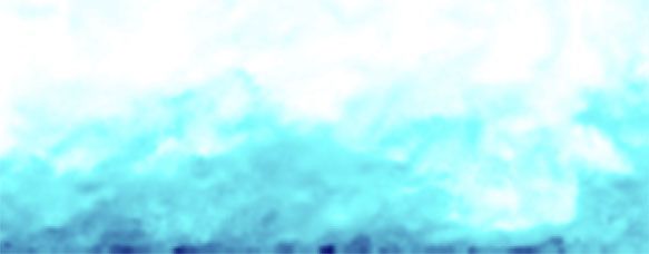
Downloaded from https://www.cambridge.org/core. IP address: 46.4.80.155, on 11 Jul 2021 at 11:15:43, subject to the Cambridge Core terms of use, available at https://www.cambridge.org/core/terms. https://doi.org/10.1017/jfm.2021.102
R. J. Hearst and others
x+
(b) –2000 0 2000 4000 6000
(a)
250 7000 1.1
6000 1.0
200
5000
0.9
y (mm)
Ũ/U∞
150 4000
y+
0.8
100 3000
0.7
2000
50 0.6
1000
0 0 0.5
–100 –50 0 50 100 150 200
x (mm)
Figure 2. (a) Camera arrangement and (b) captured field of view. The black dashed area is the investigated
region in the present study. The full field of view was investigated in the study by Dogan et al. (2019).
3. Flow characterisation
Dogan et al. (2016, 2017) and Hearst et al. (2018) explored the effects of FST on a TBL
in detail with hot-wire anemometry, including cases FST-8 and FST-13 used here. The
same cases were later explored in greater depth by Dogan et al. (2019) through the same
PIV data used herein. In this section, some key differences between the canonical TBL
case (REF) and the two FST cases are highlighted. Particular emphasis is placed on
instantaneous effects; see Dogan et al. (2016, 2017) for details on the single-point statistics
and amplitude modulation, and Dogan et al. (2019) for statistical information on the spatial
data. The minor discrepancies in the reported length scales and Reynolds numbers between
the previous and present work are related to the difference in measurement techniques used
to measure the flow and minor changes to the definitions of certain parameters.
Instantaneous streamwise velocity, denoted Ũ, snapshots of the flow field with and
without FST are presented in figure 3(a–c), which reveals clear qualitative differences in
the flows. Specifically, for the canonical case (REF), the TBL is characterised by a velocity
deficit near the wall that decreases with increasing y until the freestream, where the flow
moves uniformly at U∞ (with very minor fluctuations). On the other hand, the two FST
cases are markedly different as they both exhibit a velocity deficit region near the wall,
however, the flow above this region is composed of patches of Ũ > U∞ and Ũ < U∞ . In
this sense, the concept of U∞ exists only as the mean of the instantaneous fluctuations in
the freestream velocity, and does not describe a coherent region instantaneously. While this
result is expected, it will play largely into the analysis that follows. This result also makes it
difficult or impossible to instantaneously separate the freestream from the boundary layer
using the local seeding approach (because information is needed for the freestream as well)
or instantaneous homogeneity approach (because the freestream is not instantaneously
homogeneous) of Reuther & Kähler (2018).
The mean velocity profiles normalised by outer variables are presented in figure 3(d)
for each case. When comparing the canonical REF profile to that of FST-8 and FST-13,
it is evident that the boundary layer has become ‘fuller’ with the addition of FST;
here we use the term ‘fuller’ to describe the situation where there is more streamwise
momentum closer to the wall. The same phenomenon was identified by Hearst, Gomit &
915 A109-6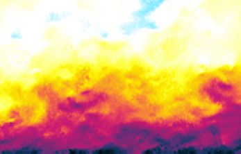
Downloaded from https://www.cambridge.org/core. IP address: 46.4.80.155, on 11 Jul 2021 at 11:15:43, subject to the Cambridge Core terms of use, available at https://www.cambridge.org/core/terms. https://doi.org/10.1017/jfm.2021.102
UMZs in a boundary layer subjected to FST
(a) 1.4 (b) (c) (d ) (e)
1.2
1.0
0.8
y/δ
0.6
0.4
0.2
0 0.25 0.50 0 0.25 0.50 0 0.25 0.50 0.6 0.8 1.0 1 10
x/δ x/δ x/δ U/U∞ (u/U)/(u∞/U∞)
Ũ/U∞
0.25 0.50 0.75 1.00 1.25 1.50 1.75
Figure 3. Instantaneous streamwise velocity flow fields for (a) REF, (b) FST-8 and (c) FST-13. Profiles of the
(d) mean velocity, and (e) turbulence intensity normalised by the FST intensity. For (d,e), (—) REF, (−−, red)
FST-8 and (− · −, blue) FST-13.
Ganapathisubramani (2016) who used FST to adjust the boundary layer profile in a study
focussing on the wake of cubes.
The representation in figure 3(d) may lead to the impression that δ is smaller for the
FST cases, however, the opposite is true. Table 1 indicates that as u∞ /U∞ is increased,
δ grows. Here, the boundary layer thickness (δ) is defined as the height at which the
mean turbulence intensity profile (u /U) is within 1 % of the turbulence intensity in the
freestream (u∞ /U∞ ); profiles of the turbulence intensity are given in figure 3(e). This
boundary layer definition was chosen because a traditional δ0.99 definition based on the
mean profiles did not produce an estimate of the boundary layer thickness that captured
the entirety of the region influenced by the wall and iterative methods – such as that of
Perry & Li (1990), which was used by Dogan et al. (2016) – could not be used effectively
due to insufficient near-wall resolution to converge the integral scheme. The present δ
estimation approach was also adopted by Dogan et al. (2019).
The boundary layer profiles normalised by wall units were presented by Dogan et al.
(2019), and figure 2(a) therein shows results from both the present PIV and earlier hot-wire
anemometry; these are shown to be in good agreement. In general, the law of the wall is
observed for the cases with FST that agree with DNS and canonical TBL measurements
from the wall up until the start of the wake region. The wake region is destroyed by the
presence of FST. Details on the inner-unit-normalised velocity profiles and the wake are
topics of other works (Dogan et al. 2016, 2017, 2019; Hearst et al. 2018), and are not
discussed further here.
We previously remarked that the instantaneous distribution of velocity in the freestream
was one of the major differences between canonical TBLs and the cases with FST. This
is illustrated in figure 4 where instantaneous fields of the signed (by vorticity) swirling
strength, λs , are provided for each case; the contours plotted in this figure as well as a
deeper analysis of λs will be addressed later in this work. For REF, all swirling strength
is contained near the wall and is predominantly signed by the wall (i.e. clockwise rotation
in the present coordinate system results in λs < 0). For the two FST cases, there is a
915 A109-7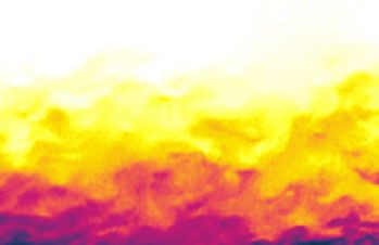
Downloaded from https://www.cambridge.org/core. IP address: 46.4.80.155, on 11 Jul 2021 at 11:15:43, subject to the Cambridge Core terms of use, available at https://www.cambridge.org/core/terms. https://doi.org/10.1017/jfm.2021.102
R. J. Hearst and others
(a) x (mm) (b) x (mm) (c) x (mm)
0 15.2 30.4 0 44.0 88.0 0 45.6 91.10 λ̃s
1.4
0.04
1.2
1.0 0.02
0.8
y/δ 0
0.6
0.4 –0.02
0.2
–0.04
0 0.25 0.50 0 0.25 0.50 0 0.25 0.50
x/δ x/δ x/δ
Figure 4. Instantaneous signed swirling strength fields for (a) REF, (b) FST-8 and (c) FST-13. The black
contour line marks the top edge of the upper-most UMZ.
region near the wall where the swirling strength is predominantly signed by the wall,
but as one moves up into the freestream there is an equal distribution of clockwise and
counter-clockwise swirl. Thus, if one is in search of an instantaneous limit to the boundary
layer, one cannot use an approach where the limit is associated with approximately zero
enstrophy because there is enstrophy instantaneously in the freestream.
4. Detection methodologies
4.1. Detecting the top of the UMZs
de Silva et al. (2016) identified that it is important to remove velocity vectors associated
with the freestream when using a histogram-based approach to detect the UMZs within
the boundary layer. The reason for this is that the freestream presents as a large UMZ and
some low velocity vectors within it mask the instantaneous histogram of the flow near
the wall. In their work, vectors above the turbulent/non-turbulence interface (TNTI) were
removed from the modal velocity analysis. The TNTI can alternatively be thought of as
the top of the upper-most UMZ in the flow. This is the context in which we approach the
problem as our entire flow is turbulent. In the present study, if vectors associated with the
freestream flow are not removed, then the high levels of turbulence in the freestream mask
any zonal structure in the boundary layer (Appendix A).
The problem of identifying the limiting contour for UMZ detection for a TBL with
a turbulent freestream has actually already been addressed by Laskari et al. (2018) for
a freestream with 3 % turbulence intensity and we follow a similar approach. They
used a modified form of the kinetic energy deficit approach of Chauhan et al. (2014a);
915 A109-8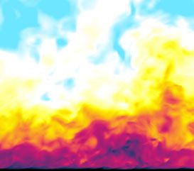
Downloaded from https://www.cambridge.org/core. IP address: 46.4.80.155, on 11 Jul 2021 at 11:15:43, subject to the Cambridge Core terms of use, available at https://www.cambridge.org/core/terms. https://doi.org/10.1017/jfm.2021.102
UMZs in a boundary layer subjected to FST
Chauhan, Philip & Marusic (2014b), who defined the kinetic energy deficit as,
1
1
k̃ = 100 × 2
[(Ũm,n − U∞ )2 + Ṽm,n
2
], (4.1)
9U∞
m,n=−1
where ˜· denotes an instantaneous quantity, the indices represent position in the PIV field
and the sum is in effect an average over a 3 × 3 window. Laskari et al. (2018) redefined
the thresholding of k̃ to accommodate the significant background energy in the freestream
by setting it to be at a level where the intermittency profile became constant (but not
necessarily 0) above δ. Without this step, their TNTI statistics were significantly different
from those measured in earlier studies.
In this spirit, we investigated the effect of several threshold levels on the present analysis.
Figure 5(a) shows contours drawn at six arbitrary threshold levels (1.0 ≤ kth /k∞ ≤ 6.0)
over a normalised instantaneous kinetic energy deficit map (k̃/k∞ ) for FST-8 (which is a
representative example of all cases); k∞ is the mean value of k̃ in the freestream across
all images and positions for a particular case. The figure illustrates that despite changes
in the threshold of 60 %, 100 %, 300 %, 400 % and 500 %, the instantaneous contours are
still grouped into only two distinct sets. The higher three thresholds are grouped together
closer to the surface than the lower three thresholds which are grouped farther from the
wall. Between them is an area of approximately uniform momentum. Figure 5(b) identifies
that the reason for this preferential positioning of the contours near each other is a result of
their alignment with shear events. In effect, the contour lines trace a path from one shear
event to the next across the field of view. Similar observations were made by Adrian et al.
(2000, figure 17), Eisma et al. (2015, figure 3) and de Silva et al. (2016, figure 4), and have
been discussed or hypothesised in a general sense for some time, e.g. Hunt & Carruthers
(1990), Hunt & Durbin (1999) and Hunt et al. (2011). It should be noted though that the
shear events that the contours track are discontinuous, and thus while the contours connect
the shear events, they do not represent a continuous shear event.
In figure 6, probability density functions (p.d.f.s) are presented for the location of the
contours for the same thresholding levels as above. The figure illustrates that, while the
variation in the contour position does change as a function of kth , its most common position
(i.e. the peak in the p.d.f.) is relatively fixed for a 500 % increase to the threshold value
for the FST cases; consider that the y-axis is a log scale. Specifically, for the illustrated
threshold levels (1.0 ≤ kth /k∞ ≤ 5.0), the peak in the instantaneous distribution of the
contour for the FST cases is relatively insensitive to kth , changing by 0.03δ for the worst
case.
This phenomenon of the alignment of contours along shear events and subsequent
mean position insensitivity highlights a certain degree of robustness in the analysis, i.e.
a degree of leniency with respect to the selection of a threshold level can be taken without
influencing the conclusions drawn in the present work. This is discussed in greater detail
in Appendix A. This realisation echoes the sentiment that the threshold is in fact a range
rather than a specific value as stated explicitly by Wu et al. (2019) and implicitly by Borrell
& Jiménez (2016) and Watanabe, Zhang & Nagata (2018).
A key difference between the REF case and the FST cases is that a continuous contour is
not guaranteed to exist for every threshold level in the flows with FST. This is illustrated for
various thresholds in figure 7, which shows the percentage of snapshots with a continuous
contour across a 0.5δ field of view at a given threshold level. For REF, thresholds in the
range 4 ≤ kth /k∞ ≤ 150 occur in every snapshot. However, no kth results in a continuous
contour in all snapshots for the FST cases. Maxima exist at kth /k∞ = 1.6 for FST-8
915 A109-9
Downloaded from https://www.cambridge.org/core. IP address: 46.4.80.155, on 11 Jul 2021 at 11:15:43, subject to the Cambridge Core terms of use, available at https://www.cambridge.org/core/terms. https://doi.org/10.1017/jfm.2021.102
R. J. Hearst and others
(a) 0.20
40
35
0.15 30
25
k̃/k∞
y/δ
0.10 20
15
0.05 10
5
0
0 0.25 0.50
(b) 0.20 8
7
0.15 6
(∂Ũ/∂y)(δ/U∞)
5
y/δ
4
0.10
3
2
0.05
1
0
0 0.25 0.50
x/δ
Figure 5. Instantaneous (a) kinetic energy deficit and (b) wall-normal shear fields with continuous contours
at kth /k∞ = 1.0, 1.6, 2.0, 4.0, 5.0 and 6.0 with increasing thresholds being the lines closer to the wall.
REF FST-8 FST-13
100
1.2
1.1
10–1
yi /δ
1.0
0.9
0.8
0.7
0.6
10–2 0.5
0.4
0 1 2 3 4
0 5 10 0 5 10 0 5 10
p.d.f. p.d.f. p.d.f.
Figure 6. The p.d.f.s of the instantaneous location of the interface for different threshold levels: kth /k∞ = 1,
1.6, 2, 3, 4 and 5 (from darkest to lightest). The selected threshold level is identified with a thicker line.
915 A109-10Downloaded from https://www.cambridge.org/core. IP address: 46.4.80.155, on 11 Jul 2021 at 11:15:43, subject to the Cambridge Core terms of use, available at https://www.cambridge.org/core/terms. https://doi.org/10.1017/jfm.2021.102
UMZs in a boundary layer subjected to FST
100
% of images with continuous contour at kth
90
80
70
60
50
40
30
20
10
0
10–1 100 101 102 103
kth/k∞
Figure 7. Percentage of images that a continuous contour exists at kth over a 0.5δ window for (—) REF, (−−,
red) FST-8 and (− · −, blue) FST-13.
with the threshold existing in 96.5 % of snapshots, and kth /k∞ = 1 for FST-13 with the
threshold existing in 88.2 % of snapshots.
Given that for the FST cases the most likely position of the contour is not strongly
dependent on kth /k∞ (figure 6), and the instantaneous contours tend to cluster in
approximately the same location for several threshold levels (figure 5), we select the
threshold level kth /k∞ to be the value that represents the most common contour in
the present measurements; i.e. kth /k∞ = 1.6 for FST-8 and kth /k∞ = 1.0 for FST-13.
Similarly, for consistency, we choose the lowest threshold value that occurs in 100 % of the
snapshots for REF, i.e. kth /k∞ = 4.0. These contours represent events that occur the most
frequently in the present dataset and in fact also result in the detection of the most UMZs in
the boundary layer region (Appendix A). The selected contours are highlighted in figure 6
and instantaneous examples of their variation for a ±50 % change in thresholding value
are presented in figure 8. In the latter figure, it can be seen that the instantaneous location
of the contour does not significantly change for at least a ±30 % change in threshold
and is still broadly in a similar position for even a ±50 % change. The changes that are
perceptible do not result in the isolation of a new UMZ, and thus do not significantly
influence that analysis. Moreover, the variation in the mean position of the identified
contour with thresholding level is small compared to the typical thickness of a UMZ, e.g.
> 0.1δ (Laskari et al. 2018). Nonetheless, it is important to note that it is the general trends
between cases that we seek to address with this analysis rather than specific quantitative
reporting.
4.2. Detecting UMZs
UMZs layered above the wall were detected using a similar methodology to that described
by Adrian et al. (2000), de Silva et al. (2016) and Laskari et al. (2018). The steps used
herein are:
915 A109-11Downloaded from https://www.cambridge.org/core. IP address: 46.4.80.155, on 11 Jul 2021 at 11:15:43, subject to the Cambridge Core terms of use, available at https://www.cambridge.org/core/terms. https://doi.org/10.1017/jfm.2021.102
R. J. Hearst and others
0.5 0.6 0.7 0.8 0.9 1.0
Ũ /U∞
(a) 0.85
REF
0.80
y/δ
0.75
0.70
(b) 0.20
FST-8
0.15
y/δ
0.10
0.05
(c) FST-13
0.15
y/δ 0.10
0.05
0 0.1 0.2 0.3 0.4 0.5
x/δ
Figure 8. Instantaneous velocity maps for all cases with the identified top edge of the upper-most UMZ drawn
in red. Additional contours are drawn for a ±10 %, 20 %, 30 %, 40 % and 50 % change in the thresholding value
in decreasing shades of grey as a reference for the variation of the contour with thresholding value.
(i) A window with a streamwise length of 2000 viscous units (L+ x = 2000) in the centre
of each vector field is selected; L+ x was chosen based on the analysis of de Silva
et al. (2016), who suggested that it should scale with viscous units. They further
showed that for Reτ 14 500 the average number of UMZs detected, NUMZ , for
a canonical TBL was approximately invariant for 200 L+ x 2500. The effect of
changing L+ x in the present study is discussed in the next section.
(ii) A p.d.f. is composed from the streamwise velocity vectors in a given image as
depicted on the right-hand side of figure 9.
(iii) Vectors above the most common continuous contour (identified in § 4.1) are excluded
from the p.d.f.s; without this step, the turbulent variations in the freestream dwarf
the wall-bounded flow for the FST cases (Appendix A).
(iv) Modal velocities of the UMZs, UUMZ , are identified as the peaks in the p.d.f. and
thresholds are drawn at the mid-point between two adjacent modal velocities to
detect the edges of the UMZs (de Silva et al. 2016).
915 A109-12Downloaded from https://www.cambridge.org/core. IP address: 46.4.80.155, on 11 Jul 2021 at 11:15:43, subject to the Cambridge Core terms of use, available at https://www.cambridge.org/core/terms. https://doi.org/10.1017/jfm.2021.102
UMZs in a boundary layer subjected to FST
0.2 0.4 0.6 0.8 1.0
Ũ/U∞
(a) REF (b)
1200 0.7 4.0
1000 0.6 3.5
3.0
800 0.5
y/δ
2.5
p.d.f.
y+ 0.4
600 2.0
0.3
400 1.5
0.2 1.0
200 0.1 0.5
0 0 0
(c) FST-8 0.25 (d)
1200 4.0
1000 0.20 3.5
3.0
800
y+ 0.15 2.5
p.d.f.
y/δ
600 2.0
0.10
400 1.5
1.0
200 0.05
0.5
0 0 0
(e) (f)
1200 FST-13 4.0
0.20 3.5
1000
3.0
800 0.15
y+ 2.5
p.d.f.
y/δ
600 2.0
0.10
400 1.5
0.05 1.0
200
0.5
0 0
0 250 500 750 1000 1250 1500 1750 2000 0.2 0.4 0.6 0.8 1.0
x+ U/U∞
Figure 9. Sample instantaneous snapshots of streamwise velocity with corresponding p.d.f.s for each of the
three test cases. The peaks in the p.d.f.s are circled, and the thresholds are drawn equidistant from the adjacent
p.d.f. peaks. These thresholds are drawn onto the instantaneous velocity fields to identify the UMZs.
When the thresholds from step (iv) are mapped onto the instantaneous velocity field
(figure 9), it can be seen that the modal velocities represent the local velocity in regions
of approximately uniform momentum. It is important to note that the UMZs detected
using this methodology are only those that form a layered structure above the wall.
There is evidence that regions of uniform momentum also exist in homogeneous isotropic
turbulence detached from a wall (Elsinga & Marusic 2010), but this is not the focus herein.
5. Impact of freestream turbulence on uniform momentum zones
Earlier works showed that the spectrograms, amplitude modulation and spatial correlations
functions of the wall-bounded flows subjected to FST are qualitatively similar to those in
canonical TBLs (Dogan et al. 2016, 2017, 2019; Hearst et al. 2018). This leads us to wonder
if the instantaneous structure near the wall is also comparable between the canonical case
915 A109-13Downloaded from https://www.cambridge.org/core. IP address: 46.4.80.155, on 11 Jul 2021 at 11:15:43, subject to the Cambridge Core terms of use, available at https://www.cambridge.org/core/terms. https://doi.org/10.1017/jfm.2021.102
R. J. Hearst and others
6
5
4
NUMZ
3
2
1
0 500 1000 1500 2000 2500 3000 3500
L+x
Figure 10. The influence of window size on the estimation of the number of UMZs in the frame. The vertical
dashed line represents the value of L+
x used to estimate the UMZ statistics herein; (− −) REF, (−−, red)
FST-8, (−−, blue) FST-13.
and ones with FST. To address this question, we search for UMZs which are markers of
the hairpin mechanisms that produce low- and high-momentum pathways in TBLs (Adrian
et al. 2000).
Figure 9 is a single example of the flow fields in each case, but it illustrates some of the
global trends present in these flows. All the flow field axes are set to represent an area that
is x+ = 2000 by y+ = 1300, and the right-hand axis of the flow fields corresponds to outer
units. The results reveal that in both viscous and outer units the UMZs are housed closer
to the wall with increasing FST; this agrees with figure 6 and is discussed in greater detail
in § 6. The closer proximity of the UMZs to the wall in both inner and outer units, despite
the slight increase in Reτ with u∞ /U∞ , suggests that this trend is robust to these changes
in Reτ and is an effect of the presence of the FST. Perhaps more significantly, UMZs are
observed for all three cases despite the fact that they occupy successively less physical
space with increasing FST. This emphasises the robustness of the zonal-like arrangement
of velocity present in wall-bounded flows, as they exist even in this flow with significant
turbulence away from the wall.
As remarked in previous works on the topic, the analysis of UMZs and their detection is
dependent on the criteria used to identify them (de Silva et al. 2016; Laskari et al. 2018).
In practice, this means that more emphasis should be placed on the trends identified in the
analysis rather than the specific values of its output. A parameter with significant impact
on the present analysis is the length of the interrogation window (Lx ). The dependence of
NUMZ on Lx is presented in figure 10. While NUMZ is approximately invariant for L+ x >
500 for the canonical REF case, in agreement with de Silva et al. (2016), there is a strong
dependence of NUMZ on Lx for the FST cases. Nonetheless, the trends when comparing
the cases to one-another are unaffected by the size of the chosen window, i.e. NUMZ
decreases with increasing FST intensity regardless of the chosen Lx . The fact that NUMZ
continues to decrease with increasing Lx for the FST cases but not for the canonical case
suggests that the physical extent of the UMZs is shorter when FST is present.
While figure 9 provides a picture of the instantaneous structure for the three cases, more
meaning can be drawn from the statistics accumulated across all fields acquired in the
present experiment. In figure 10, the general trend observed for all detection parameters
tested is that NUMZ decreases with increasing u∞ /U∞ . Specifically, for the chosen
parameters: NUMZ = 3.9, 2.0 and 1.8, for REF, FST-8 and FST-13, respectively. More
information on the detected UMZs is given by the p.d.f.s of NUMZ for the three cases,
915 A109-14Downloaded from https://www.cambridge.org/core. IP address: 46.4.80.155, on 11 Jul 2021 at 11:15:43, subject to the Cambridge Core terms of use, available at https://www.cambridge.org/core/terms. https://doi.org/10.1017/jfm.2021.102
UMZs in a boundary layer subjected to FST
(a) (b)
0.50 11
0.45 10
0.40 9
0.35 8
7
0.30
p.d.f.
6
0.25
5
0.20
4
0.15 3
0.10 2
0.05 1
0
0 1 2 3 4 5 6 7 8 0.4 0.5 0.6 0.7 0.8 0.9 1.0 1.1 1.2 1.3
NUMZ NUMZ /U∞
Figure 11. The p.d.f.s of the (a) number of UMZs and (b) normalised modal velocities for each case; (− −)
REF, (−−, red) FST-8, (−−, blue) FST-13.
illustrated in figure 11(a). The peak of the p.d.f. moves from 4, to 2 to 1, for increasing
u∞ /U∞ . Significantly, there are always more fields with NUMZ ≥ 2 than NUMZ < 2 for
all cases, suggesting that UMZs do exist in these flows. It is also worthwhile to note that
there are recorded fields where NUMZ = 0 instantaneously for FST-8 and FST-13, but not
REF. NUMZ = 0 for the FST cases identifies fields where continuous contours across the
field of view could not be detected. This occurs in 0 %, 3.5 % and 11.8 % of the acquired
images for REF, FST-8 and FST-13, respectively, again demonstrating that in the majority
of realisations UMZs are detected.
The p.d.f.s of the modal velocities (UUMZ ) for each case are provided in figure 11(b).
This figure illustrates the likelihood that a UMZ with a given modal velocity will exist
in a given instantaneous field. The first prominent feature of this figure is the maximum
for each case that decreases in UUMZ /U∞ for increasing u∞ /U∞ . This is an artefact of
the thresholds used to identify the upper-most edge of the UMZs, and simply identifies
that there is typically a UMZ with the same momentum as the threshold. What is perhaps
more interesting in figure 11(b) is that the p.d.f.s are very similar for UUMZ /U∞ < 0.75.
The significance of this is it identifies that the distribution of modal velocities is practically
unchanged by the presence of the FST. This in turn tells us that the primary impact of the
FST is to reorganise the outer regions of the boundary layer, while leaving the near-wall
structure intact. This thus corroborates the results from the spectra (Dogan et al. 2016;
Hearst et al. 2018) and amplitude modulation (Dogan et al. 2017) analyses that conclude
that qualitatively the near-wall structure of the flows is unaffected (other than the change
in Uτ ).
6. The upper-most UMZ edge
In the previous section it was demonstrated that UMZs exist near the wall for TBLs
subjected to FST in much the same way as they do for canonical TBLs. We now turn our
attention to what happens where the UMZs stop. In particular, we focus on the top edge
of the upper-most UMZ, representing the last continuous contour that exists when moving
away from the wall. In principle, this is a similar idea to the TNTI, which separates the
UMZs from the freestream for a canonical TBL, however, FST above the TBL means the
flow is completely populated by turbulence. Thus, the top edge of the UMZs is likely more
915 A109-15Downloaded from https://www.cambridge.org/core. IP address: 46.4.80.155, on 11 Jul 2021 at 11:15:43, subject to the Cambridge Core terms of use, available at https://www.cambridge.org/core/terms. https://doi.org/10.1017/jfm.2021.102
R. J. Hearst and others
similar to an internal shear layer within the TBL (Eisma et al. 2015), or the interfaces
demarking the quiescent core of a channel (Kwon et al. 2014; Yang et al. 2016; Jie et al.
2019) or central UMZ of a pipe (Chen et al. 2020; Gul et al. 2020) than to a TNTI. An
interface separating the wall turbulence over a flat plate from FST above it has previously
been detected by Wu et al. (2019) who referred to it as the ‘boundary layer turbulence and
freestream turbulence interface’. While their interface was not framed in the same way,
it provides a precedent that a meaningful contour exists that distinguishes wall-bounded
turbulent structures from the flow above.
As was qualitatively demonstrated in figures 3(a–c), 4 and 9, the instantaneous velocity
deficit and wall-signed vorticity regions, as well as the UMZs themselves, all appear
to be contained closer to the wall for the FST cases compared to the canonical case.
Figure 12(a) shows the p.d.f.s of the location of the top UMZ edge for the three cases,
explicitly illustrating that it statistically moves closer to the wall with increasing FST.
Figure 12(a) also identifies some key differences between the three cases. For REF, the
p.d.f. is approximately Gaussian, as observed in previous studies for the TNTI of canonical
TBLs (Chauhan et al. 2014a; Eisma et al. 2015). However, for the two FST cases, the
distributions are markedly skewed towards the wall. This links directly to differences
in the intermittency, γ , profiles provided in figure 12(b). The intermittency profiles are
calculated by creating a binary field for each velocity field where 1 is assigned to all
vectors in the UMZ region (below the upper-most UMZ edge) and 0 is assigned to all
values that are not part of the UMZs. Taking the average of these fields yields the curves
provided in figure 12(b), where γ = 1 represents flow that is always occupied by UMZs
and γ = 0 represents flow that is never occupied by UMZs. The intermittency profile for
REF is approximately an error function in agreement with previous studies, e.g. Chauhan
et al. (2014a). The error function parameterisation does not hold for the FST cases. This
means that there are instantaneous flow fields that have no UMZs. Moreover, γ > 0 until
y/δ ≈ 1.4 for the FST cases, suggesting that there is significant variability in the position
of the top edge of the UMZs for these cases. In particular, if the p.d.f.s in figure 12(a)
are integrated from the peak value up, it demonstrates that 86.7 % and 94.6 % of the time
the top of the UMZs is above the peak location of the p.d.f. for cases FST-8 and FST-13,
respectively. This is in sharp contrast to REF where the peak in the p.d.f. is essentially
the centre of the distribution. In all, the p.d.f.s and intermittency profiles in figure 12
demonstrate that the top edge of the UMZs moves closer to the wall with increasing FST
and that its positional variability increases with FST.
If the top edge of the upper-most UMZ is truly a contour of significance, then one would
expect to see jump flow characteristics across it (Wu et al. 2019). This is assessed through
conditional averages taken about the aforementioned contour. In general, we focus on the
differences and similarities for cases FST-8 and FST-13. The REF results are omitted from
this section because the Reτ is much lower. For detailed investigations on canonical TBLs
and the effect of Reτ in those flows, see Chauhan et al. (2014a,b) and de Silva et al. (2017).
The conditional averages are calculated by conditioning the wall-normal position, y on the
position of the upper-most UMZ edge, yi , i.e. y − yi = 0 is the position of the UMZ edge.
Each vertical profile from each image for a specific case is then averaged in this way. In
figure 13(a), mean velocity jumps across the top UMZ edge are illustrated for the FST
cases, similar to observations for canonical TBLs made by Chauhan et al. (2014b). The
change in slope of the profile of Ũi above and below the contour is greater for FST-13
compared to FST-8, suggesting that the severity of the discontinuity is a function of the
FST intensity and is higher than the canonical case. In order to quantify this, linear fits
were made to the various sections of the curve in figure 13(a) to illustrate the change to the
915 A109-16Downloaded from https://www.cambridge.org/core. IP address: 46.4.80.155, on 11 Jul 2021 at 11:15:43, subject to the Cambridge Core terms of use, available at https://www.cambridge.org/core/terms. https://doi.org/10.1017/jfm.2021.102
UMZs in a boundary layer subjected to FST
(a) (b)
1.4 1.4
1.2 1.2
1.0 1.0
yi /δ
0.8 0.8
y/δ
0.6 0.6
0.4 0.4
0.2 0.2
0 0.5 1.0 1.5 2.0 2.5 3.0 3.5 4.0 4.5 0 0.1 0.2 0.3 0.4 0.5 0.6 0.7 0.8 0.9 1.0
p.d.f. γ
Figure 12. Wall-normal profiles of the (a) p.d.f. of the location of the upper-most UMZ edge, yi , and (b) the
intermittency, γ , profile for each case; (− −) REF, (−−, red) FST-8, (−−, blue) FST-13.
(a) 0.05 (b)
0.05
0.04 0.04
0.03 0.03
0.02 0.02
( y − yi)/δ
0.01 0.01
0 0
–0.01 –0.01
–0.02 –0.02
–0.03 –0.03
–0.04 –0.04
–0.05 –0.05
–0.08 –0.06–0.04 –0.02 0 0.02 0.04 0.06 0.08 –6 –4 –2 0 2 4 6 8 10 12
(×10–3)
(Ũ i – Ui)/U∞ Ṽ i /U∞
Figure 13. Conditional averages across the instantaneous location of the top edge of the upper-most UMZ:
(a) mean streamwise velocity and (b) mean wall-normal velocity; (−−, red) FST-8, (−−, blue) FST-13.
velocity jump across the upper edge of the top UMZ, D[Uτ ]. Chauhan et al. (2014b) found
that for sufficient Reτ the velocity jump, D[Uτ ], was approximately invariant for canonical
TBLs. We measure D[Uτ ] ≈ 1.87 and 1.94 for cases FST-8 and FST-13, respectively.
This confirms that increasing the FST has the function of increasing the velocity jump
across the top edge of the upper-most UMZ. This idea is also consistent with the notion
that increasing the FST makes the boundary layer ‘fuller’. Wu et al. (2019) composed
conditional averages across their interface but their conditional averages were performed
in the interface-normal direction rather than the wall-normal direction. Nonetheless, their
results also show a velocity jump, albeit less severe than presented here. Their FST was
closer to 3 % and thus their results support the hypothesis that the velocity jump scales
with the FST intensity when combined with the present findings.
The conditional wall-normal velocity profile is similar to that observed for the canonical
cases (Chauhan et al. 2014a) in that below the interface the flow direction is away from the
wall, while above the interface fluid is entrained down, consistent with the idea that flow is
entrained down into the turbulent wall region. The difference between the cases presented
915 A109-17Downloaded from https://www.cambridge.org/core. IP address: 46.4.80.155, on 11 Jul 2021 at 11:15:43, subject to the Cambridge Core terms of use, available at https://www.cambridge.org/core/terms. https://doi.org/10.1017/jfm.2021.102
R. J. Hearst and others
(a) (b)
0.05 0.05
0.04 0.04
0.03 0.03
0.02 0.02
( y − yi)/δ
0.01 0.01
0 0
–0.01 –0.01
–0.02 –0.02
–0.03 –0.03
–0.04 –0.04
–0.05 –0.05
–0.06 –0.05 –0.04 –0.03 –0.02 –0.01 0 –1.0 –0.9 –0.8 –0.7 –0.6 –0.5 –0.4 –0.3
λ̃i ũṽi /U 2τ
Figure 14. Conditional averages across the instantaneous location of the top edge of the upper-most UMZ:
(a) signed swirling strength and (b) Reynolds shear stress; (−−, red) FST-8, (−−, blue) FST-13.
here is that the incoming and exiting profiles are more uniform for FST-13 relative to
FST-8, again suggesting that a stronger discontinuity is present for the increased level of
FST.
Further insight into the mechanics at the edge of the UMZs can be obtained from
the conditionally averaged swirling strength signed by vorticity, which is provided in
figure 14(a). Below the top UMZ upper edge the swirl is negative, while it approaches
zero above the highest UMZ. The results for the two different turbulence levels are similar,
and the conditional statistics corroborate the qualitative observation made with respect to
figure 4 that above the UMZs there is an approximately equal distribution of positive and
negative vortices while below there is a bias towards the wall-signed vorticity. This adds
further weight to the idea that the identified threshold represents a physically meaningful
interface that demarcates the two flow regions because statistically these isolines behave
in a similar way to one identified directly with vorticity. Note that a fundamentally similar
results was presented by Wu et al. (2019) for their slightly different conditional averaging
process.
The conditionally averaged Reynolds shear stress is shown in figure 14(b) where a peak
is visible at the upper-most UMZ edge contour. The fluctuating velocities are estimated in
the usual sense where they are the difference between the mean field and the instantaneous
field. Of note is that the u v profile through the contour more closely resembles the internal
layers detected by Eisma et al. (2015) than the TNTI profile of Chauhan et al. (2014a).
Moreover, Wu et al. (2019) also found that their interface was a local peak in the Reynolds
shear stress. This result is consistent with the idea that there is turbulence and mean shear
on both sides of the contour, which results in production.
The general picture painted by the UMZ analysis and observations made on the edge
of the upper-most UMZ is that the primary impact of the FST is on the outer regions
of the boundary layer. Specifically, with increasing FST, the top of the highest UMZ is
pushed towards the wall and there is less area for the boundary layer structure or UMZs
to manifest. Increasing u∞ /U∞ results in an increase in Reτ , primarily via a change in δ
as the changes to Uτ between cases are around 5 % while δ changes by a factor of three
(table 1). In a canonical TBL an increase in Reτ is correlated to an increase in NUMZ (de
Silva et al. 2016), however, the present analysis demonstrates that increasing u∞ /U∞ also
915 A109-18Downloaded from https://www.cambridge.org/core. IP address: 46.4.80.155, on 11 Jul 2021 at 11:15:43, subject to the Cambridge Core terms of use, available at https://www.cambridge.org/core/terms. https://doi.org/10.1017/jfm.2021.102
UMZs in a boundary layer subjected to FST
brings the top of the highest UMZ closer to the wall, and that NUMZ decreases. Thus,
one can conclude that the impact of the FST on the outer regions of the boundary layer
is more significant for the instantaneous structure of the boundary layer than the increase
in Reτ . This may initially seem at odds with the idea that the presence of FST causes δ
to grow, however, it is important to note that Chauhan et al. (2014a) also found that the
TNTI (for canonical TBLs) lay below δ at approximately 23 δ. As such, the present results
could be interpreted as FST causing an increase to the size of the intermittent region
between the edge of the boundary layer, δ, and the interface bounding the UMZs. This
is explicitly demonstrated in figure 12(b). Regardless, UMZs exist for FST levels up to
u∞ /U∞ = 12.8 %, which, in combination with earlier spectral (Dogan et al. 2016; Hearst
et al. 2018), amplitude modulation (Dogan et al. 2017) and spatial correlation (Dogan et al.
2019) results, suggests that the primary impact of changing u∞ /U∞ is to change the outer
regions of the boundary layer while approximately preserving the near-wall region flow
features.
7. A simplified model of a boundary layer with freestream turbulence
The interaction between FST and a TBL is extremely complex, and measurements at any
specific downstream location are in fact a result of the integrated influence of the two
flows on one another over the entire development length up to the measurement point
(Kozul et al. 2020; Jooss et al. 2021). Based on our observations so far, it is evident that a
TBL with FST appears to show characteristics of the superposition of two turbulent flows.
Specifically, we observe a region close to the wall that exhibits purely TBL characteristics,
while above the UMZs we observe an altered structure resulting from the presence of
FST. Even farther away from the wall, the flow behaves purely as FST. In order to test this
hypothesis, we aim to utilise a simple model where we superimpose an isotropic turbulence
field over a TBL to see if the preceding trends are reproducible.
7.1. Model formulation
This idea was realised by superimposing instantaneous fields from a scaled periodic
turbulent box (Cao, Chen & Doolen 1999) – accessed through the John Hopkins
Turbulence Database – on the turbulent boundary layer DNS of Sillero, Jiménez & Moser
(2013, 2014) at Reτ = 2000. Functionally, this was accomplished by interpolating the
isotropic DNS fields to an equivalent grid as the TBL DNS and then scaling the velocity
magnitudes based on the turbulence intensity of the empirical FST for each case. Blending
was performed in two ways: (i) by simply superimposing the two fields, and (ii) by using
the empirical intermittency profiles (figure 12b) as a relative weighting between the two
flows. The subsequent figures are shown using approach (ii), however, the results did not
substantially differ between the two approaches. The synthetic field generation process is
illustrated in figure 15 for approach (ii) and the output image is qualitatively similar to
those for cases FST-8 and FST-13 in figure 3. Particularly, the freestream is composed of
packets of velocity that are both Ũ < U∞ and Ũ > U∞ , and there is a velocity deficit
region near the wall. One hundred synthetic images were generated to mirror each of the
experimental datasets (REF, FST-8, FST-13), and the modelled flows are referred to as
mREF, mFST-8 and mFST-13, respectively. The 100 fields for each case are composed
of the same baseline TBL fields, and differ only in that isotropic fields with varying
magnitudes are superimposed on to them. To this end, the approach isolates the effects
of FST in that mFST-8 and mFST-13 differ only in the magnitude of the superimposed
turbulent field, but not in their instantaneous boundary layer or freestream structure;
915 A109-19You can also read