MLCTR: A Fast Scalable Coupled Tensor Completion Based on Multi-Layer Non-Linear Matrix Factorization
←
→
Page content transcription
If your browser does not render page correctly, please read the page content below
MLCTR: A Fast Scalable Coupled Tensor Completion Based on Multi-Layer
                                                              Non-Linear Matrix Factorization

                                              Ajim Uddin∗             Dan Zhou∗            Xinyuan Tao∗            Chia-Ching Chou†                 Dantong Yu∗

                                        Abstract
                                        Firms earning prediction plays a vital role in investment de-
arXiv:2109.01773v1 [cs.LG] 4 Sep 2021

                                        cisions, dividends expectation, and share price. It often in-
                                        volves multiple tensor-compatible datasets with non-linear
                                        multi-way relationships, spatiotemporal structures, and dif-
                                        ferent levels of sparsity. Current non-linear tensor comple-
                                        tion algorithms tend to learn noisy embedding and incur
                                        overfitting. This paper focuses on the embedding learning
                                        aspect of the tensor completion problem and proposes a new         Figure 1: Tensor completion on the Earning Per Share
                                        multi-layer neural network architecture for tensor factoriza-      (EPS) data. The accuracy of tensor completion with
                                        tion and completion (MLCTR). The network architecture              low-rank decomposition severely degenerates with in-
                                        entails multiple advantages: a series of low-rank matrix fac-      creasing tensor sparsity. In contrast, our algorithm
                                        torizations (MF) building blocks to minimize overfitting, in-      with the coupled tensor factorization maintains accu-
                                        terleaved transfer functions in each layer for non-linearity,      racy even with 99.13% of missing values.
                                        and by-pass connections to reduce the gradient diminishing
                                        problem and increase the depths of neural networks. Fur-           (Reconstruction). Over the years, a number of low-rank
                                        thermore, the model employs Stochastic Gradient Descent            tensor completion methods have been proposed [Acar
                                        (SGD) based optimization for fast convergence in training.         et al., 2011a, Gandy et al., 2011, Song et al., 2017, Liu
                                        Our algorithm is highly efficient for imputing missing values      et al., 2018,Wu et al., 2019b,Liu et al., 2019]. These ex-
                                        in the EPS data. Experiments confirm that our strategy of          isting algorithms suffer two mutually exclusive problems
                                        incorporating non-linearity in factor matrices demonstrates        in achieving the two objectives. First, linear low-rank
                                        impressive performance in embedding learning and end-to-           algorithms [Acar et al., 2011a, Gandy et al., 2011, Song
                                        end tensor models, and outperforms approaches with non-            et al., 2017]) attain low-rank embedding matrices by
                                        linearity in the phase of reconstructing tensors from factor       Singular Value Decomposition (SVD), but fail to cap-
                                        matrices.                                                          ture the multi-way (non-linear) relationships that are
                                           Keywords: Sparse Tensor Completion, Nonlinear                   common in real-world tensor applications. The lack of
                                        Coupled Tensor Factorization, Finance.                             multi-way relationship modeling results in suboptimal
                                                                                                           performance in tensor completion or downstream pre-
                                        1    Introduction                                                  diction [Fang et al., 2015, He et al., 2014, Zhe et al.,
                                                                                                           2016].
                                        Tensor completion algorithms are mostly based on
                                                                                                                Second, algorithms with nonlinear reconstruction
                                        two representative low-rank tensor factorization mod-
                                                                                                           (e.g., [Liu et al., 2018,Wu et al., 2019b,Liu et al., 2019])
                                        els: CANDECOMP/PARAFAC (CP) [Harshman et al.,
                                                                                                           focus on nonlinear relationship learning among factors
                                        1970] and Tucker [Tucker, 1966]. These approaches at-
                                                                                                           and use “kernel tricks” or neural network layers to repre-
                                        tempt to identify low-rank factor matrices using the ob-
                                                                                                           sent the embedding factors and multi-way relationships.
                                        served entries and then reconstruct the target tensor
                                                                                                           When multi-way relationship learning becomes domi-
                                        based on these factors matrices. The low-rank tensor
                                                                                                           nant, it ignores the structure of input signals, makes no
                                        completion essentially boils down to a two-step problem
                                                                                                           constraints on factor matrices, and attempts to encode
                                        with two objectives: representation learning (Factoriza-
                                                                                                           all information signal into the relationships. The lack of
                                        tion) and subsequent multi-way relationship prediction
                                                                                                           data structure in embedding matrices will lead to low-
                                           ∗ New Jersey Institute of Technology, Newark, NJ, USA. {au76,
                                                                                                           quality embeddings that are prone to noise, variance,
                                        dz239, xinyuan.tao, dtyu}.njit.edu
                                                                                                           and overfitting.
                                           † Central Michigan University, Mount Pleasant, MI, USA.              In this paper, we design a multi-layer matrix factor-
                                        chou1c@cmich.edu                                                   ization neural networks for coupled tensor reconstruc-

                                                                                                                                              Copyright © 20XX by SIAM
                                                                                                                       Unauthorized reproduction of this article is prohibited
(a) CP (b) CoSTCo (c) MLCTR
Figure 2: The quarters and firms embedding matrix learned from (a) CP based factorization, (b) CoSTCo, and
(c) MLCTR. The factors in both CP and MLCTR are much more clear and concise than CoSTCo. Especially,
the time embedding factors clearly demonstrate patterns in the high frequency band and low frequency band
and captures the yearly business cycles (8 peaks and trough for 32 quarters) and US economic recovery from
2011-2012 onward (MLCTR 6th and 7th factors). In CP and MLCTR factorization, almost all information is
forced to pass through the embedding matrices, whereas in CoSTCo the CNN of the later part also captures a
significant portion of tensor information, resulting in less informative embedding matrices.
tion (MLCTR). MLCTR learns the distributed repre- modified objective function for element-wise reconstruc-
sentations effectively for prediction and multi-way rela- tion and SGD optimization. To confirm the MLCTR al-
tionship tasks. Unlike existing nonlinear tensor comple- gorithm’s superiority, we evaluate it on finance datasets
tion methods, it avoids the difficult trade-off between and three other commonly used public data sets, in-
the two tensor completion objectives and introduces cluding climate and point of interest (POI) data. The
non-linearity in the embedding learning step. It explic- experiment results reveal the consistency and reliability
itly employs Multi-Layer matrix factorization for factor of our model. The main contributions of our paper are
matrices and uses nonlinear transfer functions in each as follows:
layer, thereby learning the highly complex structures
and relationship among the hidden variables. Besides, • We develop a novel nonlinear coupled tensor com-
to avoid the vanishing gradient in the deep architecture, pletion model based on multi-layer matrix factor-
we use by-pass connection following [He et al., 2016]. ization, nonlinear-deep neural networks, and by-
The resulted architecture has less reconstruction error pass connections to efficiently learn both embed-
(Fig. 1) and generates high-quality embedding matrix ding matrix and nonlinear interaction between the
(Fig. 2). embedded vectors.
Figure 1 also shows the sparsity problem with ten- • The learned embeddings encode latent data struc-
sor completion: as the number of missing observations tures and patterns and provide high-quality dis-
increases, the accuracy decreases significantly. With our tributed representation for downstream machine
proposed model, we can easily mitigate this problem by learning tasks.
augmenting sparse data sets with auxiliary data. Lit-
erature suggest auxiliary information from a secondary • We propose the first-ever SGD based nonlinear
dataset significantly improves tensor completion accu- coupled tensor completion algorithm that is fast
racy [Narita et al., 2012, Kim et al., 2017, Acar et al., and scalable.
2011b, Bahargam and Papalexakis, 2018]. We take
• We introduce the by-pass connection to mitigate
advantage of data structures among multiple tensors,
the gradient diminishing problem in networks with
apply tensor integration mechanism as appropriate to
great depths.
reduce the associated computation cost, and scale-up
MLCTR to factorize two or more coupled sparse ten-
2 Related Work
sors simultaneously.
Our coupled tensor completion algorithm uses a 2.1 Tensor Completion In recent years, a number
of low-rank tensor completion algorithms [Gandy et al.,
Copyright © 20XX by SIAM
Unauthorized reproduction of this article is prohibited2011, Liu et al., 2012, Song et al., 2017, Acar et al., 3 Methodology
2011a] are developed based on classical CP [Harshman Tensor factorization can be formulated as a two-step
et al., 1970] and Tucker factorization [Tucker, 1966]. paradigm: embedding learning and subsequent rela-
The low-rank approach is not always precise and of- tionship modeling. In contrast to the majority of
ten fails to capture frequent nonlinear interactions in tensor algorithms that focus on non-linear relation-
real-world applications. To capture real-world nonlin- ship modeling in the second step, MLCTR considers
ear relationships, in [Liu et al., 2018, Wu et al., 2019b], the first embedding learning step and explicitly guides
authors replace multi-linear operation with multi-layer networks to learn representative vectors for each en-
perceptions (MLP) and in [Liu et al., 2019] authors tity. The MLCTR learns the embedding matrix and
proposed a convolution neural network-based architec- multi-way interaction among the embeddings with the
ture. Nevertheless, these works try to learn the low- same stack of networks. The approach has a con-
rank representation of single tensor and do not con- nection to the kernel-based support vector machine.
sider any auxiliary information to improve the factor The well-known Radial Basis Function Kernel (RBF)
matrices. In [Narita et al., 2012, Kim et al., 2017], essentially is an infinite sum over polynomial ker-
authors introduce regularization from auxiliary data nels, each of which can be further expanded to lin-
and demonstrate performance improvement. In recent ear dot products in the polynomial space. The RBF
years, coupled matrix-tensor factorization (CMTF) also kernel defines a high-dimensional transform ΨRBF :
gains broad interests [Acar et al., 2011b, Bahargam and KRBF (x, y) = hΨRBF (x), ΨRBF (y)i. An appropriate
Papalexakis, 2018]. CMTF factorizes a higher-order embedding transformation Ψ approximates non-linear
tensor with a related matrix in a coupled fashion. Unlike kernels with linear dot products among embedding vec-
CMTF, our approach is a coupled tensor factorization tors, and thus, greatly simplify the downstream rela-
for sparse data where both data sets are higher-order tionship learning. The embedding learning algorithm
tensors. There are several coupled tensor factorization starts with a random signal and adds incrementally new
approaches available [Khan et al., 2016, Genicot et al., information into the embedding vectors in multi-layered
2016, Wu et al., 2019a]; however, these models are not network architecture in Figure 3.
designed for sparse data and require a full observation
in both tensors. Compared to this, our MLCTR relaxes 3.1 Multi-Layer Model for Tensor Factoriza-
the constraints of complete observations and captures tion We adopt Multi-Layer matrix factorization to con-
non-linearity in both target tensors. struct the factor matrices of the tensor, thereby learn-
ing meaningful embeddings. Given a factor matrix
2.2 EPS Forecast for Estimating Firm’s Earn- U ∈ Rd1 ×r , U = [u1 , u2 , · · · , ud1 ]> is a collection of
ings Expected EPS conveys the vital information d1 embeddings with r dimensions. The factor matrix
about firms’ future cash flows and is one of the criti- holds the feature vectors of d1 entities. Their feature
cal inputs for security pricing [Lee and So, 2017]. The vectors presumably have structure and are generated
current industry benchmark averages across all available from H hidden variables in l different groups (clusters).
analysts’ forecasts for each firm at each quarter. How- For simplicity, we assume that each group uniformly has
ever, studies suggest that this straightforward average h = Hl hidden variables. For example, the real space im-
forecast has several drawbacks: it may contain system- age features might originate from different groups of hid-
atic bias [Ramnath et al., 2008, Bradshaw et al., 2012] den variables: frequency bands, pose features, color fea-
and fail to incorporate additional information from mar- tures, expression features, and identify features. Based
kets, firm characteristics, analysts features, and crowd- on this preassumption, we further decompose U into two
sourcing [Bradley et al., 2017, Ball and Ghysels, 2018]. hidden matrices P and Q and learn the feature grouping
To address these problems, the authors in [Bradley structure simultaneously as follows:
et al., 2017] assign different weights among analysts
based on their past performance. More efforts of [Corre- l−1
X
dor et al., 2019, Bradshaw et al., 2012] show that the (3.1) U = Pd1 ×H QH×r = P (j) × Q(j) ,
model combining accounting characteristics with ana- j=0
lysts’ EPS forecast generates better earning predictions
where P (j) = [pjh , pjh+1 , · · · , pjh+h−1 ]> and Q(j) =
than the widely adopted time-series models do. Our
[qjh , qjh+1 , · · · , qjh+h−1 ]> . When the group informa-
work entails a novel data mining approach MLCTR to
tion is known, we explicitly arrange the order of hidden
explore a new avenue of analyzing financial data, es-
variables and provide a group-aware matrix factoriza-
pecially with tensor representation and missing value
tion, as shown in the right hand in Eqn 3.1. In most
imputation.
cases, the group information and hidden variables are
Copyright © 20XX by SIAM
Unauthorized reproduction of this article is prohibitedFigure 3: In the Multi-Layer Network Ar-
chitecture for Learning Embedding, we use
by-pass connections to create very deep
networks (up to 34 layers in this exam-
ple) to learn complex data structures. The
multi-way relationships among all factors
are modeled by the linear dot product. We
can also use MLP or convolutional neu-
ral networks and trade-off the complexity
between the embedding layers and rela-
tionship modeling layers. This architec-
ture mitigates the overfitting problem by
adding structural constraints in the high-
dimensional embedding.
unknown, and nevertheless can be extracted by our pro- where the input matrix at layer 0 is zero, and the
posed multi-layer matrix factorization networks. inputs to the multi-linear dot product in the right-hand
The multi-layer matrix factorization has the funda- side of Figure 3 is U (out) = U (l−1) . Figure 3 shows
mental connection to signal processing: the Q(j) con- P (j) and Q(j) are the trainable parameters, and their
sists of the base (loading) vectors of transformation (for products are applied with non-linear transfer functions
example, Fourier or Spectral transformation) and P (j) before and after being added into the forward path
is the loading scores of U on the base matrix Q(j) , i.e., from the lower layer to the higher layer. The network
the row vectors in U are the weighted sum of the base has a by-pass connection from the layer input directly
signals in different frequency bands. We do not assume to the layer output and applies element-wise matrix
any prior knowledge of the bands of hidden variables additions to implement identity mapping. Similar to the
and treat data as the signals from different frequency ResNet [He et al., 2016], the by-pass connection design
bands. Here, each rank of the matrix factorization P does not increase the number of neurons and mitigates
and Q represents one frequency band. We will use the the problem of gradient vanishing and explosions that
j-th layer neural network in Figure 3 to learn the P (j) often occur in networks with a great depth. The
and Q(j) in Eqn 3.1 and attempt to extract h related fre- multiple layers of matrix factorization and by-pass
quencies in the same band simultaneously. The dimen- greatly enhance the modeling capacity for non-linearity,
sonality of U at different layer is the same (U j ∈ Rdi ×r while incurring no higher training errors than those
and U j−1 ∈ Rdi ×r ), which helps to remove noises and without it.
learn meaningful signal without forcing the model to 3.3 Coupled Tensor Factorization for Embed-
compress the available information. ding Learning and Prediction Nearly all ten-
Given the complicated relationship embedded in U , sor completion algorithms, including our proposed
this multi-layer approach partitions the learning into MLCTR, often suffer the cold start problem and ex-
l frequency bands. Each frequency band corresponds tremely low signal to noise ratio (SNR) [Acar et al.,
to a network layer in Figure 3. This design eases 2012]. Especially in our finance application, the EPS
the complexity associated with single layer and avoids dataset has a high number of missing values, i.e., 99%.
the complexity of learning to model the entire signal The time, analyst, and f irm latent factors learned from
altogether. the EPS tensor are less informative because of the ex-
cessive number of miss values. To recover the critical
3.2 Non Linearity and By-pass Connection We missing signal, we introduce additional data synergistic
introduce non-linear transfer functions σ, i.e., ReLU, to the EPS tensor to be imputed. The firm fundamen-
ELU, and sigmoid, in the factor matrix U and its tals share the same time and firm dimensions with EPS
corresponding multi-layer neural network of Eqn 3.1. and provide complementary information for any firm
We rewrite non-linear matrix factorization in each layer in EPS, including key performance indicators and firm
j as follows: characteristics.
In the coupled tensor framework, MLCTR attempts
to enforce the same time factor and firm factor matrices
during factorization. The information propagates from
(3.2) U (j) = σ(U (j−1) + σ(P (j) × Q(j) )),
Copyright © 20XX by SIAM
Unauthorized reproduction of this article is prohibitedAlgorithm 1: MLCTR Coupled
Input : Tensor X ∈ Rd1 ×d2 ×d3 and tensor
Y ∈ Rd1 ×d2 ×d4 to be completed, rank
of tensor decomposition r, rank of
matrix factorization h, network
layers l, index set of observed entries
ΩX in the tensor X and ΩY in the
tensor Y.
Output: Updated factor matrices
U (0) , V (0) , W (0) , T (0) and hidden
matrices P (j) and Q(j)
(j = 0, . . . , l − 1)
1 Initialize all hidden matrices P (j) and Q(j) for
Figure 4: Coupled Tensor Factorization and Completion
all layers, initialize U (0) , V (0) , W (0) , T (0)
2 repeat The objective function for coupled tensor is to minimize
3 for α = ∀(i, j, k) ∈ ΩX ∪ ΩY do the mean square error of two tensor factorizations by
// Forward Propagation optimizing the following equation:
4 for j ← 1 to l − 1 do 2
5 U (j) = σ(U (j−1) + σ(P (j) × Q(j) )) (3.3) L = X − [[Λ1 ; U (out) , V (out) , T (out) ]] F
Similarly, calculate V, W, T ; // Eqn 2
6 +λ Y − [[Λ2 ; U (out) , V (out) , W (out) ]] F
3.2
7 Calculate loss L ; // Eqn 3.4
Here λ is the hyper-parameter to adjust the relative
// Backward Propagation
importance between the two coupled tensors. The
8 if α ∈ ΩX then factors matrices T (out) , U (out) , V (out) , W (out) are the
9 Update U (0) , V (0) , T (0) and output of the multi-layer embedding learning networks.
associated P (j) and Q(j) based on
3.4 SGD-based Coupled Tensor Factorization
chain rule and Eqn. 3.5.
and Integration Traditional CMFT requires complete
10 else
tensors for factorization and incurs long computation
11 Update all U (0) , V (0) , W (0) and
time for large tensors. In this paper, we perform an
associated P (j) and Q(j) based on element-wise tensor reconstruction from the observation
chain rule and Eqn. 3.5. set Ω for fast convergence. We revise the objective
12 until maximum number of epochs or early function as follows to be compatible with any deep
stopping; neural network platform:
(3.4)
r
1ΩX (ijk) Xijk − (out) (out) (out) 2
X X
the dense tensor (firm accounting fundamentals) to L= Uis Vjs Tks F
the sparse tensor (analysts’ EPS forecast) by coupling i,j,k∈ΩX ∪ΩY s=1
r
the firm and time factors in tensor factorization and
+λ1ΩY (ijk) Yijk −
X (out) (out) (out) 2
completion. Figure 4 describes the MLCTR system for Uis Vjs Wks ) F
,
s=1
coupled tensor, factorizing two tensors: X and Y, each
of which has three factor matrices: two common factor where 1ΩX (ijk) is an indicator function. It is straight-
matrices U and V and the unique matrix T for X and forward to implement Eqn 3.4 with the Stochastic Gra-
W for Y. We assume all factor matrices have the same dient Descent (SGD): we first mix the training data from
rank r. Figure 4 shows a simple linear dot product ΩX and ΩY , randomly choose one mini-batch of training
for multi-way relationship. Alternatively, we add MLP samples, and calculate the mean square error defined in
between the embedding learning layer and the output Eqn 3.4. This mixing strategy intelligently employs in-
layer for modeling addition non-linear relationships.1 dicator functions to allow any observation to be treated
uniformly, thereby enabling the parallel processing of
1 In the experiment part, we call MLCTR for using simple dot the samples in the same mini-batch. Eqn 3.4 essentially
product and MLCTR (MLP) for using MLP layers between the is multi-task learning and thereby highly scalable to al-
middle layer and output layer on the architecture. low multiple tensors to be factorized simultaneously.
Copyright © 20XX by SIAM
Unauthorized reproduction of this article is prohibitedFor any training sample, the gradient of the first Table 1: Data statistics and Hyper-parameters
term or the second term in Eqn. 3.4 is zero. Considering Datasets shape observed entries lr batch size
the sample with index (i, j, k) ∈ ΩX , we calculate the SafeGraph (6439, 6439, 365) 95509754 1e-4 8192
corresponding gradient of L to the embeddings and SafeGraph (log10) (6439, 6439, 365) 95509754 1e-4 8192
update the relevant parameters as follows:
(3.5)
(out) (out) original CBG, destination CBG and date with shape
Ui,: ← Ui,: 6439 × 6439 × 365. To ensure a reasonable data dis-
r
(out) (out) (out) (out) (out) tribution, we apply the log transformation and use the
X
− η( Uis Vjs Tks − Xijk )(Vj,: Tk,: ) grid search to find the proper base as 10.
s=1
In addition, we test the efficiency of our algorithm
Here is the Hadamard product of two vectors. The on two commonly used public datasets. The first
gradients on other factor matrices V, W, T have the iden- one is climate data, which is used in [Lozano et al.,
tical formula to Eqn 3.5. We only show the parameter in 2009, Liu et al., 2010]. The dataset has 18 climate
matrix U . The gradient is back-propagated through the agents from 125 locations from 1992-2002. The second
network layers in Figures 3 and 4. Algorithm 1 shows one is a real point of interest (POI) data used in [Li
the pseudo-code of SGD based MLCTR2 . et al., 2015]. The Foursquare check-in data made in
Singapore between Aug. 2010 and Jul. 2011. The
4 Experiments data comprises 194,108 check-ins made by 2,321 users
We conduct two experiments for four datasets to eval- at 5,596 POI. Using two different processing systems,
uate our algorithm: 1) efficiency in tensor completion we develop two different tensor representations of the
in both time and accuracy compared to other state- POI dataset, i.e., POI and POI-3D. For POI we follow
of-the-art tensor completion techniques and 2) ability the approach used in [Liu et al., 2019] and represent
to factorize sparse coupled tensor while learning mean- the tensor as (user id, poi id, location id). The first
ingful factor matrix. To alleviate the overfitting prob- two dimensions user id and poi id are available in
lem, we try several regularization methods inlcudung data, in [Liu et al., 2019], the authors created the
Lasso, Ringe, and Elaticnet and call these models as third dimension ‘location id’ by splitting the POIs into
Resnet-L1, Resnet-L2, Resnet-Elastic. We compare our 1600 location clusters based on their respective latitude
algorithm with CPWOPT [Acar et al., 2011a] - the and longitude. Hence, both 2nd-order and 3rd-order
benchmark low-rank sparse tensor completion method, represent location information, and for each location id,
P-Tucker [Oh et al., 2018] - a scalable Tucker model with we have different poi id, resulting in an unnecessary
fully paralleled row-wise updating rule, and CoSTCo large tensor. In POI-3D we overcome this limitation
[Liu et al., 2019] - CNN based state-of-the-art nonlinear by incorporating time information available in the data
tensor completion method. To evaluate performance, and replace location id with time to represent tensor as
we use three metrics, RMSE, MAE, and MAPE. (user id, poi id, time). We divide the 24 hours into 12
groups of 2 hours intervals. This incorporation of time
4.1 Data We apply our MLCTR for SafeGraph information helps us learn a better latent representation
Foot Traffic data. SafeGraph collects cellphone of user probability of visiting a specific POI at a specific
GPS location data from a panel of cellphone time.
users when a set of installed apps are used and We normalize the datasets with zero mean and unit
they are available for free to academics study- variance. For EPS and climate data, we use an 80/20
ing COVID-19 (https://www.safegraph.com/covid-19- train-test split, with 10% of the training data as the
data-consortium). These cellphone GPS location data validation set and early-stopping if validation loss does
are supplied at the daily level for residents of each Cen- not improve for 10 epoch. For both POI datasets, we use
sus Block Group(CBG). In the following experiment We the train-validation-test set following [Li et al., 2015].
collect 95509754 records belonging to five boroughs of The tensor shape, number of observed entries for each
New York States (The Bronx, Brooklyn, Manhattan, of the data sets, and Hyper-parameters are reported in
Queens, and Staten Island.) for the sample period of Table 1.
2019. And we use these records to construct a three
order tensor to describe the three-way relationship of 4.2 Coupled Tensor Completion We fac-
torize two sparse tensors –analysts’ EPS forecast
2 We will publish the Python notebooks in GitHub for repro- (quarter, f irm, analyst) and firm fundamentals
ducibility. (quarter, f irm, f undamental)– together with the ob-
Copyright © 20XX by SIAM
Unauthorized reproduction of this article is prohibitedTable 2: Tensor Completion Result
Metric RMSE MAE MAPE
Data Model/rank 10 20 30 40 10 20 30 40 10 20 30 40
CPWOPT 0.3865 0.3434 0.3352 0.4171 0.1735 0.1722 0.2274 0.2137 35.7778 36.2522 32.3325 39.8641
EPS and P-Tucker 0.3364 0.3106 0.2954 0.2802 0.2173 0.1934 0.1755 0.1406 34.7840 32.1949 29.1234 28.0701
Fundamentals CoSTCo 0.2536 0.2364 0.2455 0.2310 0.1337 0.1338 0.1185 0.1096 29.7298 30.4989 26.4746 24.0901
MLCTR 0.3229 0.2900 0.1947 0.1818 0.1678 0.1457 0.0984 0.0946 31.4561 28.6817 21.7898 21.1656
MLCTR (MLP) 0.2645 0.2140 0.1940 0.1996 0.1385 0.1078 0.0979 0.0914 27.6427 22.2719 21.1212 19.4139
MLCTR (Coupled) 0.2421 0.2065 0.1703 0.1520 0.1355 0.1016 0.0810 0.0806 24.2524 18.9695 16.6764 17.4226
CPWOPT 0.4155 0.3636 0.3363 0.3294 0.2694 0.2144 0.1869 0.1754 94.4968 94.3807 87.7374 86.0715
Climate P-Tucker 0.4231 0.3746 0.3224 0.3201 0.2844 0.2417 0.1942 0.1648 104.4845 98.7135 78.4751 75.5421
CoSTCo 0.3955 0.3040 0.3019 0.2577 0.2676 0.2022 0.1991 0.1667 59.7978 47.7849 47.4389 39.6156
MLCTR 0.3750 0.3023 0.2543 0.2326 0.2501 0.1953 0.1625 0.1434 55.7723 44.1495 37.9093 33.3923
MLCTR (MLP) 0.3558 0.2902 0.2572 0.2410 0.2378 0.1897 0.1679 0.1551 54.2780 45.0224 40.5167 37.5005
P-Tucker 0.2464 0.2182 0.1989 0.1784 0.1484 0.1443 0.1204 0.1182 84.1285 81.4561 72.9842 70.9242
POI CoSTCo 0.1536 0.1532 0.1535 0.1534 0.0887 0.0877 0.0883 0.0849 54.8782 53.5907 54.4279 49.9463
MLCTR 0.1532 0.1534 0.1531 0.1533 0.0883 0.0819 0.0878 0.0846 54.5828 47.1175 54.1197 50.0688
MLCTR (MLP) 0.1539 0.1538 0.1536 0.1541 0.0833 0.0829 0.0829 0.0826 48.1277 47.5316 47.5259 46.8857
P-Tucker 0.1814 0.1784 0.1441 0.1403 0.1103 0.1017 0.0987 0.0915 57.0812 46.9813 42.7891 39.8714
POI-3D CoSTCo 0.1064 0.1056 0.1057 0.1052 0.0543 0.0517 0.0521 0.0497 36.0018 33.5342 33.9658 31.1371
MLCTR 0.1084 0.1088 0.1064 0.1064 0.0564 0.0566 0.0559 0.0571 37.1333 37.1333 37.2212 38.3884
MLCTR (MLP) 0.1051 0.1053 0.1058 0.1052 0.0486 0.0504 0.0535 0.0495 30.2706 32.1058 35.3082 31.0428
(a) Convergence Plot (b) Rank vs Accuracy
Figure 5: (a) Convergence plot of MLCTR (Coupled)
for EPS data. (b) Tensor completion accuracy at Figure 6: Similarity heatmap among “quarters” factors.
different ranks for EPS data.
jective function of eq. 3.4. For imputing missing values, factors can also learn better embedding for single ten-
coupled tensor factorization produces much higher sor. To show such generalization of MLCTR, we con-
accuracy than single factorization. As reported in duct analysis using three public datasets. On climate
Table 2, MLCTR (coupled) can outperform CPWOPT forecasting, MLCTR outperforms CPWOPT, P-Tucker,
by 49% (rank = 30, best performing CPWOPT) and and CoSTCo in all three performance metrics (Table 2).
CoSTCo by 34%(rank = 40, best performing CoSTCo). At rank 30, MLCTR (MLP) outperforms CPWOPT by
The benefits of coupled tensor completion beyond 24%, P-Tucker by 20% and CoSTCo by 15% in RMSE.
single tensor completion can be captured by the per- For both POI datasets, the data sparsity is too high.
formance improvement between MLCTR and MLCTR With only 0.0005% (POI) and 0.09% (POI-3D) available
coupled. With rank 40, MLCTR (coupled) outperforms observation, CPWOPT with gradient descent does not
MLCTR (MLP) by 16% (RMSE), 15% (MAE) and converge. Therefore, for POI data, we did not report
18% (MAPE). The proposed MLCTR algorithm is also the CPWOPT result. In POI, with rank 30, MLCTR
robust to the increasing number of missing values. As (MLP) outperforms P-Tucker by 31%, and CoSTCo by
shown in Figure 1, even with 99% missing values, our 13% in MAPE; whereas CoSTCo is only better at rank
algorithm can still impute missing values accurately, 10 in RMSE. For POI-3D, CoSTCo outperforms simple
outperforming CoSTCo by 37%. MLCTR is also less MLCTR in some performance metrics. However, our
sensitive to rank. Figure 5b shows that with higher MLP version MLCTR (MLP) still outperforms CoSTCo
ranks, MAPE decline smoothly for all three versions of with higher ranks (30 and 40) by a significant margin.
MLCTR.
4.4 Visualization of Learned Factors As shown
4.3 Sparse Single Tensor Completion MLCTR is in Fig. 2, the learned factor matrices from MLTCR is
not only effective for coupled tensor completion, but the much more informative than other nonlinear tensor fac-
technique of using residuals by further factorizing latent torization models. To further understand the learned
Copyright © 20XX by SIAM
Unauthorized reproduction of this article is prohibitedas input variables; therefore, it is linear to the number of
available observations rather than the size of the target
tensor. Figure 8 shows the running time of each algo-
rithm in each data sets at different ranks. The reported
time elapsed for each algorithm is with early stopping
criteria. The time complexity of MLCTR is also linear
to the rank and does not increase drastically with higher
ranks.
5 Discussion
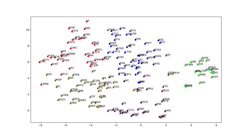
Figure 7: t-SNE and spectral clustering on learned
The proposed MLCTR algorithm divides the tensor fac-
“firm” factors.
torization and completion into two interleaved modules:
the first one that learns the rank r embeddings and the
second one for modeling multi-way relationships among
the embeddings of the participating entities. The ma-
jority of related work focuses on the latter: for an N th-
order tensor, N -way linear (including CP and Tucker
decompositions) and nonlinear kernels (RBF, polyno-
mial) are employed to model the relationships and min-
imize the mean square errors between the observations
and predicted values.
Tensor rank is the key parameter in factorizing a
tensor. The common practice is to perform a grid
search on an appropriate rank r. A small rank r in-
curs large bias in tensor analysis while a high rank r
Figure 8: Running time of different tensor completion leads to overfitting [Liu et al., 2019]. The overfitting
algorithms at different ranks. problem is primarily due to many unconstrained r hid-
den variables in embeddings and must be regularized to
factors, we visualize the factor matrices learned from minimize variance. The standard l1 and l2 regulariza-
coupled tensor factorization on analysts’ EPS forecast tions only add the local constraints of smoothness and
and firm fundamentals data. Fig. 6 shows the cosine sparsity on embeddings and might not be sufficient for
similarity between “quarters” learn from the time fac- our problem. Inspired by the signal processing theory,
tors matrix. The temporal patterns in the time fac- we introduce the structure, base constraints, and global
tors are clearly visible. Fig. ?? shows the t-distributed regularization to the embedding space. We argue that
stochastic neighbor embedding (t-SNE) to plot the spec- high-quality embedding learning will mitigate the com-
tral clustering based on firm latent factors. MLCTR plexity in the second module for relationship modeling
learns meaningful embedding for firms according to so that a simple linear dot product in CP or a shallow
their size, service type, and the client groups they serve. MLP is sufficient in the algorithmic implementation.
For example, major retail brands like Walmart (WMT),
Urban Outfitters (URBN), Gap (GPS), Abercrombie & 6 Conclusion
Fitch (ANF) are grouped Far-right (Green); major tech In this paper, we apply an innovative approach to shift
companies like Microsoft (MSFT), NVIDIA (NVDA), the learning towards the embedding module, ensuring
Amazon (AMZN), IBM, Akamai (AKAM) are grouped its central role in a tensor algorithm, and easing re-
in top-center (Blue); and financial service companies lationship learning. With the high-quality embedding,
like Fidelity (FABC), Zions Bancorporation (ZION), many multi-way relationships can be efficiently modeled
Morgan Stanley (DWD), iShares (GSG) are grouped in by the CP tensor algorithm or simple MLP networks.
bottom-center (Purple). We implement MLCTR using multi-layer neural net-
works where each layer performs low-rank matrix fac-
4.5 Running Time Comparison MLCTR uses torization for embedding matrices. Experiments show
low-rank MF and by-pass connections for learning la- that our algorithm works exceptionally well for both
tent factors; thus, it learns embedding matrix much single tensor and coupled tensor factorization and com-
faster than other nonlinear algorithms, i.e., CoSTCo, pletion and is less sensitive to tensor rank, robust to
P-Tucker. MLCTR takes indices of the observed values noise, and fast to converge during training.
Copyright © 20XX by SIAM
Unauthorized reproduction of this article is prohibitedReferences [He et al., 2016] He, K., Zhang, X., Ren, S., and Sun, J.
(2016). Deep residual learning for image recognition.
[Acar et al., 2011a] Acar, E., Dunlavy, D. M., Kolda, T. G., In Proceedings of the IEEE conference on computer
and Mørup, M. (2011a). Scalable tensor factorizations vision and pattern recognition, pages 770–778.
for incomplete data. Chemometrics and Intelligent [He et al., 2014] He, L., Kong, X., Yu, P. S., Yang, X., Ra-
Laboratory Systems, 106(1):41–56. gin, A. B., and Hao, Z. (2014). Dusk: A dual structure-
[Acar et al., 2012] Acar, E., Gürdeniz, G., Rasmussen, preserving kernel for supervised tensor learning with
M. A., Rago, D., Dragsted, L. O., and Bro, R. (2012). applications to neuroimages. In Proceedings of the 2014
Coupled matrix factorization with sparse factors to SIAM International Conference on Data Mining, pages
identify potential biomarkers in metabolomics. In 2012 127–135. SIAM.
IEEE 12th International Conference on Data Mining [Khan et al., 2016] Khan, S. A., Leppäaho, E., and Kaski,
Workshops, pages 1–8. IEEE. S. (2016). Bayesian multi-tensor factorization. Ma-
[Acar et al., 2011b] Acar, E., Kolda, T. G., and Dunlavy, chine Learning, 105(2):233–253.
D. M. (2011b). All-at-once optimization for cou- [Kim et al., 2017] Kim, Y., El-Kareh, R., Sun, J., Yu, H.,
pled matrix and tensor factorizations. arXiv preprint and Jiang, X. (2017). Discriminative and distinct phe-
arXiv:1105.3422. notyping by constrained tensor factorization. Scientific
[Bahargam and Papalexakis, 2018] Bahargam, S. and Pa- reports, 7(1):1–12.
palexakis, E. E. (2018). Constrained coupled matrix- [Lee and So, 2017] Lee, C. M. and So, E. C. (2017). Un-
tensor factorization and its application in pattern and covering expected returns: Information in analyst
topic detection. In 2018 IEEE/ACM International coverage proxies. Journal of Financial Economics,
Conference on Advances in Social Networks Analysis 124(2):331–348.
and Mining (ASONAM), pages 91–94. IEEE. [Li et al., 2015] Li, X., Cong, G., Li, X.-L., Pham, T.-A. N.,
[Ball and Ghysels, 2018] Ball, R. T. and Ghysels, E. (2018). and Krishnaswamy, S. (2015). Rank-geofm: A ranking
Automated earnings forecasts: Beat analysts or com- based geographical factorization method for point of
bine and conquer? Management Science, 64(10):4936– interest recommendation. In Proceedings of the 38th
4952. International ACM SIGIR Conference on Research and
[Bradley et al., 2017] Bradley, D., Gokkaya, S., and Liu, X. Development in Information Retrieval, pages 433–442.
(2017). Before an analyst becomes an analyst: Does [Liu et al., 2018] Liu, B., He, L., Li, Y., Zhe, S., and
industry experience matter? The Journal of Finance, Xu, Z. (2018). Neuralcp: Bayesian multiway data
72(2):751–792. analysis with neural tensor decomposition. Cognitive
[Bradshaw et al., 2012] Bradshaw, M. T., Drake, M. S., Computation, 10(6):1051–1061.
Myers, J. N., and Myers, L. A. (2012). A re- [Liu et al., 2019] Liu, H., Li, Y., Tsang, M., and Liu, Y.
examination of analysts’ superiority over time-series (2019). Costco: A neural tensor completion model
forecasts of annual earnings. Review of Accounting for sparse tensors. In Proceedings of the 25th ACM
Studies, 17(4):944–968. SIGKDD International Conference on Knowledge Dis-
[Corredor et al., 2019] Corredor, P., Ferrer, E., and Santa- covery & Data Mining, KDD ’19, page 324–334, New
maria, R. (2019). The role of sentiment and stock York, NY, USA. Association for Computing Machin-
characteristics in the translation of analysts’ forecasts ery.
into recommendations. The North American Journal [Liu et al., 2012] Liu, J., Musialski, P., Wonka, P., and Ye,
of Economics and Finance, 49:252–272. J. (2012). Tensor completion for estimating missing
[Fang et al., 2015] Fang, X., Pan, R., Cao, G., He, X., and values in visual data. IEEE transactions on pattern
Dai, W. (2015). Personalized tag recommendation analysis and machine intelligence, 35(1):208–220.
through nonlinear tensor factorization using gaussian [Liu et al., 2010] Liu, Y., Niculescu-Mizil, A., Lozano, A.,
kernel. In Twenty-Ninth AAAI Conference on Artifi- and Lu, Y. (2010). Learning temporal causal graphs
cial Intelligence. for relational time-series analysis. In Proceedings of
[Gandy et al., 2011] Gandy, S., Recht, B., and Yamada, the 27th International Conference on International
I. (2011). Tensor completion and low-n-rank tensor Conference on Machine Learning, pages 687–694.
recovery via convex optimization. Inverse Problems, [Lozano et al., 2009] Lozano, A. C., Li, H., Niculescu-Mizil,
27(2):025010. A., Liu, Y., Perlich, C., Hosking, J., and Abe, N.
[Genicot et al., 2016] Genicot, M., Absil, P.-A., Lambiotte, (2009). Spatial-temporal causal modeling for climate
R., and Sami, S. (2016). Coupled tensor decomposi- change attribution. In Proceedings of the 15th ACM
tion: a step towards robust components. In 2016 24th SIGKDD international conference on Knowledge dis-
European Signal Processing Conference (EUSIPCO), covery and data mining.
pages 1308–1312. IEEE. [Narita et al., 2012] Narita, A., Hayashi, K., Tomioka, R.,
[Harshman et al., 1970] Harshman, R. A. et al. (1970). and Kashima, H. (2012). Tensor factorization using
Foundations of the parafac procedure: Models and con- auxiliary information. Data Mining and Knowledge
ditions for an” explanatory” multimodal factor analy- Discovery, 25(2):298–324.
sis. [Oh et al., 2018] Oh, S., Park, N., Lee, S., and Kang,
Copyright © 20XX by SIAM
Unauthorized reproduction of this article is prohibitedU. (2018). Scalable tucker factorization for sparse
tensors-algorithms and discoveries. In 2018 IEEE
34th International Conference on Data Engineering
(ICDE), pages 1120–1131. IEEE.
[Ramnath et al., 2008] Ramnath, S., Rock, S., and Shane,
P. (2008). The financial analyst forecasting literature:
A taxonomy with suggestions for further research.
International Journal of Forecasting, 24(1):34–75.
[Song et al., 2017] Song, Q., Huang, X., Ge, H., Caverlee,
J., and Hu, X. (2017). Multi-aspect streaming tensor
completion. In Proceedings of the 23rd ACM SIGKDD
International Conference on Knowledge Discovery and
Data Mining, pages 435–443.
[Tucker, 1966] Tucker, L. R. (1966). Some mathematical
notes on three-mode factor analysis. Psychometrika,
31(3):279–311.
[Wu et al., 2019a] Wu, Q., Wang, J., Fan, J., Xu, G.,
Wu, J., Johnson, B., Li, X., Do, Q., and Ge, R.
(2019a). Improved coupled tensor factorization with
its applications in health data analysis. Complexity,
2019.
[Wu et al., 2019b] Wu, X., Shi, B., Dong, Y., Huang, C.,
and Chawla, N. V. (2019b). Neural tensor factorization
for temporal interaction learning. In Proceedings of the
Twelfth ACM International Conference on Web Search
and Data Mining, WSDM ’19, page 537–545, New
York, NY, USA. Association for Computing Machinery.
[Zhe et al., 2016] Zhe, S., Zhang, K., Wang, P., Lee, K.-
c., Xu, Z., Qi, Y., and Ghahramani, Z. (2016). Dis-
tributed flexible nonlinear tensor factorization. In Ad-
vances in neural information processing systems, pages
928–936.
Copyright © 20XX by SIAM
Unauthorized reproduction of this article is prohibitedYou can also read