A PRACTICAL INTRODUCTION TO THE BOOTSTRAP: A VERSATILE METHOD TO MAKE INFERENCES BY USING DATA-DRIVEN SIMULATIONS - PSYARXIV
←
→
Page content transcription
If your browser does not render page correctly, please read the page content below
A practical introduction to the bootstrap: a versatile method to make
inferences by using data-driven simulations
Guillaume A. Rousselet1, Cyril R. Pernet2, Rand R. Wilcox3
1: Guillaume.Rousselet@glasgow.ac.uk Institute of Neuroscience & Psychology, University of Glasgow, Glasgow,
Scotland, G128QB, UK

2: cyril.pernet@ed.ac.uk Centre for Clinical Brain Sciences, Neuroimaging Sciences, University of Edinburgh,
Edinburgh, UK

3: rwilcox@usc.edu Department of Psychology, University of Southern California, Los Angeles, CA, USA

Abstract

The bootstrap is a versatile technique that relies on data-driven simulations to make statistical
inferences. When combined with robust estimators, the bootstrap can afford much more
powerful and flexible inferences than is possible with standard approaches such as t-tests on
means. In this R tutorial, we use detailed illustrations of bootstrap simulations to give readers an
intuition of what the bootstrap does and how it can be applied to solve many practical problems,
such as building confidence intervals for many aspects of the data. In particular, we illustrate how
to build confidence intervals for measures of location, including measures of central tendency, in
the one-sample case, for two independent and two dependent groups. We also demonstrate how
to compare correlation coefficients using the bootstrap and to perform simulations to determine
if the bootstrap is fit for purpose for a particular application. The tutorial also addresses two
widespread misconceptions about the bootstrap: that it makes no assumptions about the data,
and that it leads to robust inferences on its own. The tutorial focuses on detailed graphical
descriptions, with data and code available online to reproduce the figures and analyses in the
article (https://osf.io/8b4t5/).

       Submitted to Meta-Psychology.

       The fully transparent Editorial process can be accessed by clicking
       here. Anyone can contribute with Open Peer Review. To do so, directly
       add comments into the PDF via hypothes.is."

                                                                                                     Page 1 of 42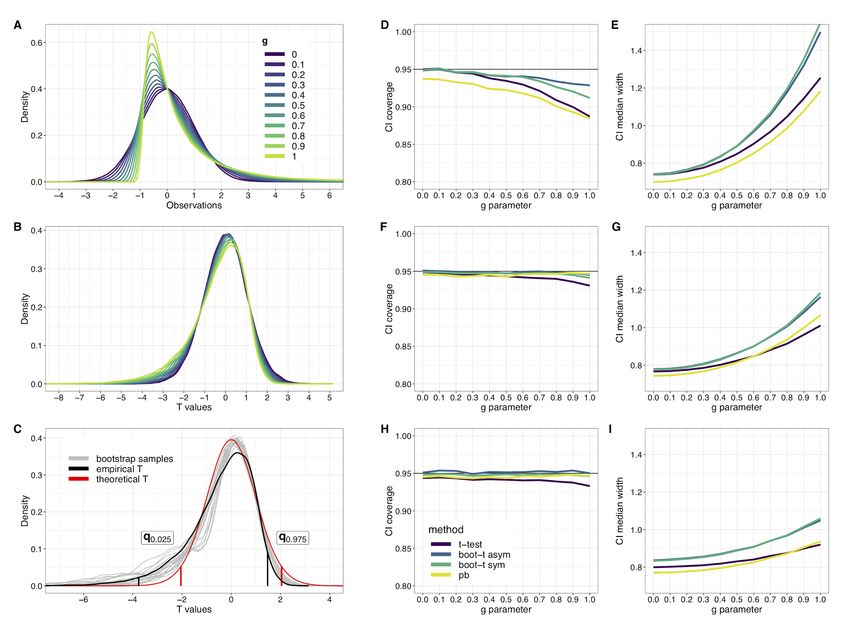
Introduction

The bootstrap is a well-established early computer-age inferential method (Efron, 1979; Efron &
Hastie, 2016; Efron & Tibshirani, 1994). The bootstrap is based on the idea that using only the
data at hand can sometimes give better results than making unwarranted assumptions about the
populations we’re trying to estimate. The core mechanism of the bootstrap is sampling with
replacement from the data, which is a form of data-driven simulation. Thus, learning about the
bootstrap is not only learning about an alternative to the standard parametric methods of
statistical inference, but is also a way to learn about simulations and to question our choices of
methods. As we will see, the bootstrap doesn’t provide a single alternative approach to classic
problems such as group comparisons, but a large family of new approaches. Having the
bootstrap in your toolbox is like getting a powerful Swiss Army Knife, which offers great
versatility—others have referred to the bootstrap as Meat Axe, Swan-Dive, Jack-Rabbit, and
Shotgun (Efron, 1979).

In this tutorial, we start by explaining the basic mechanism of the bootstrap and the rich output it
creates. We then consider the limitations of the bootstrap, before covering key applications to
inferences about group comparisons of measures of locations and correlation coefficients. We
also provide examples of simulations to quantify the long-term behaviour of the bootstrap, to
help make informed choices about statistical tools. Finally, we briefly introduce one of many
variants of the original bootstrap, the bootstrap-t technique, which has applications in analyses of
variance (ANOVAs). Other variants of the bootstrap have been proposed since 1979, such as the
wild bootstrap (Wu, 1986), the bias-corrected and accelerated bootstrap, the smooth bootstrap
(Efron & Tibshirani, 1994), and the Bayesian bootstrap (Bååth, 2015; Rubin, 1981) , to name a
few—and research into bootstrap methods is still very active.

Before we start, let’s keep in mind that for each combination of experimental design and type of
data, there is a variety of statistical analysis options available, each asking different questions, and
that no method dominates in all situations (see e.g. Rousselet, Pernet, & Wilcox, 2017; Rousselet
& Wilcox, 2019). The bootstrap is no exception: it works well in some situations but not in others.

                                                                                            Page 2 of 42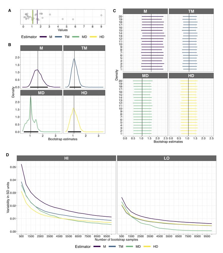
Disclosures

All the figures and analyses presented in this tutorial can be reproduced using notebooks in the R
programming language (R Core Team, 2018), as part of a reproducibility package available on
the OSF (Rousselet, Pernet, & Wilcox, 2019). All the figures are licensed CC-BY 4.0. Each figure
caption ends with the name of the RMarkdown file that can be used to reproduce it. The main R
packages used to generate the data and make the figures are ggplot2 (Wickham, 2016), cowplot
(Wilke, 2017), tibble (Müller & Wickham, 2018), facetscales (Moreno, 2019), rogme (Rousselet et al.,
2017), knitr (Xie, 2018), and the essential beepr (Bååth, 2018).

Bootstrap: the basics

Imagine we carried out an experiment and we obtained the 30 observations in Figure 1A. The
traditional approach to compute a confidence interval (CI in the rest of the text) involves a few
calculations and some parametric assumptions. First, some null value is subtracted from the
mean (let say here our null hypothesis is that the population mean is 2), and this difference is then
normalised by dividing it by the standard error of the mean (SEM). This T statistic (mean
difference/SEM) is assumed to have a particular long-run distribution determined by the sample
size (i.e. if we were to redo this experiment many times, with 30 observations, this is the
distribution we should get). This distribution, also known as a T distribution, here with 29
degrees of freedom, is illustrated in Figure 1B. The distribution assumes that we repetitively
sample from a standard normal distribution, and for each sample of size n = 30, we compute a T
value. To build a 95% CI, we read out the 2.5th quantile from that distribution and plug that
value into the CI formula (Figure 1B inset). In our example, the sample mean is 1.61 and a 95%
CI, which contains the null value, is [0.9, 2.31]. A CI for the mean is an interval that covers the
population mean with a rate of error alpha, here 5% for a 95% CI (Morey & Rouder, 2011). It
can thus be described as the interval compatible with the data, given our model (i.e. the long-run
T distribution and any other assumptions we make)—so when the model is wrong, the long-run
interval will not behave as intended (Greenland et al., 2016). We will demonstrate how to assess
the validity and quality of CIs using simulations in later sections.
                                                                                         Page 3 of 42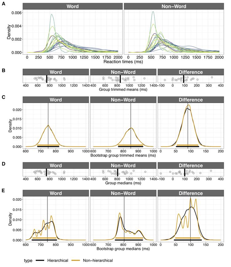
Finally, the probability of observing a result at least as extreme as our T value, given the null
long-run T distribution, is the P value (C. Pernet, 2017). Half of the P value is the area under the
curve marked in red in Figure 1B, to the left of the observed T value. To obtain the P value for a
two-sided test, the area is multiplied by two.

                                                                                          Page 4 of 42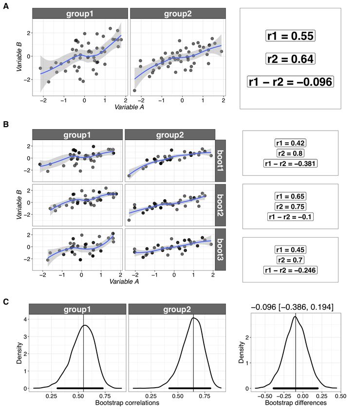
Figure 1. Percentile bootstrap inferences. A. Stripchart illustrating a random sample (n=30) from
a skewed (lognormal) distribution. Each disk is an observation. The horizontal dashed line marks the
sample median; the plain line marks the sample mean. B. Sampling T distribution for 29 degrees of
freedom. Tcrit = critical T value; Tobs = observed T value. The red area corresponds to half the P value.
The inset contains the formula for the standard T-test confidence interval. C. Bootstrap samples. Each
disk is a bootstrap observation. For each bootstrap sample, the vertical line marks the bootstrap mean. D.
Bootstrap sampling distribution of the mean. The standard deviation (SD) of the bootstrap distribution
provides an estimate of the standard error of the mean (SEM). The P value is equal to twice the minimum
between the proportion of bootstrap samples to the left and to the right of the null value (here 2), marked
by the vertical dashed line. So in this example the P value is twice the red area for a two-sided test. The
confidence interval is marked by a black horizontal line, with the values of the lower (L) and upper (U)
bounds in black labels. This figure was created using the R notebook pb.Rmd.

                                                                                               Page 5 of 42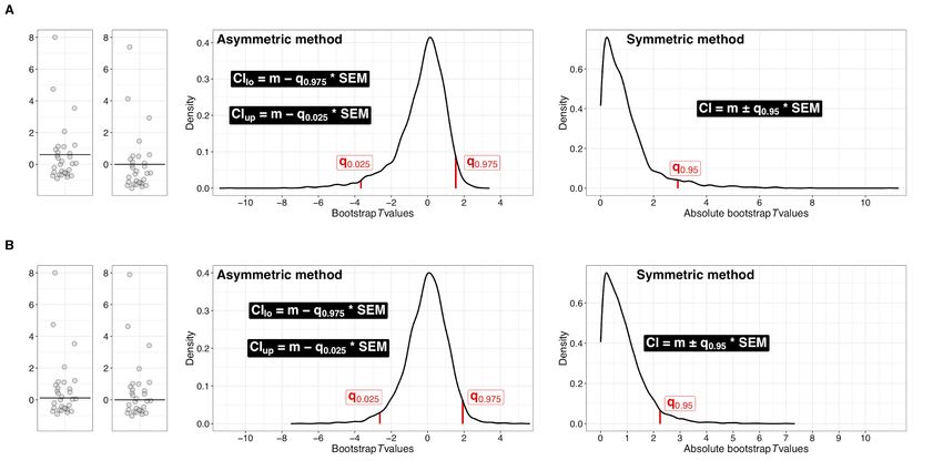
An interesting aspect from the example above is that when we use a T- test (or another
parametric test), it assumes a certain long-term distribution of the test statistics. Indeed, the
confidence interval based on the T-test relies on the long-term value of T. Suppose, for example,
that a study were repeated many times and that 2.5% of these T values are less than or equal to -
2 and 2.5% are greater than or equal to 2. Then the .95 CI would be given by the formula in
Figure 1B insert, with Tcrit= 2. Assuming normality, there is no need to determine the critical
value in this manner; the critical value can be derived exactly. But momentarily imagine that the
critical value is unknown. One could determine it by generating data from a normal distribution,
note the value of T, and repeat this process say 10,000 times. If 2.5% of these T values are less
than or equal to -2, and 2.5% are greater than or equal to 2, this indicates that Tcrit= 2. This
result is based on a particular model: random sampling from a normal distribution. Thus, long-
term T distributions used in T-tests (and F distributions in ANOVAs) represent the outcome of
virtual experiments, given a certain sample size and assuming that we sample from a population
with a particular shape. As we will see, the bootstrap-t method, described later in this article,
mimics this process. The main difference is that values are randomly sampled with replacement
from the observed data rather than from a normal distribution.

With the bootstrap, we relax parametric assumptions to instead perform data-driven simulations.
The core mechanism of the bootstrap is random sampling with replacement. To illustrate, say we
have this sample of 6 observations: 1, 2, 3, 4, 5, 6. A bootstrap sample consists of 6 observations
sampled with replacement from the original ones. Here are examples of three such bootstrap
samples:

[1] 5 2 1 6 1 1

[2] 2 6 2 5 4 4

[3] 5 6 6 6 2 2

In some bootstrap samples, some original observations are sampled more than once, others are
not sampled at all. For each bootstrap sample, we compute an estimate, say the sample mean.
So, if we take 1,000 bootstrap samples and for each of them we compute the mean, we end up
with a distribution of 1,000 bootstrap estimates of the sample mean. The key idea is that if the
                                                                                            Page 6 of 42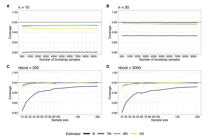
original sample size and the number of bootstrap samples are large enough, in many situations
the distribution of bootstrap estimates provides a good approximation of the sampling
distribution of the estimate.

If we go back to our Figure 1 example, panel C illustrates 20 bootstrap samples. Given our
sample size of n=30, each of these bootstrap samples contains 30 observations sampled with
replacement from the original sample. Because of random sampling, the bootstrap mean differs
across bootstrap samples. The idea is that these fluctuations represent the fluctuations expected if
we repeated the same experiment many times, each time collecting 30 new observations and
computing the mean. After 5,000 bootstraps, we obtain the distribution in Figure 1D. This
sampling distribution of bootstrap estimates is the main outcome of the bootstrap procedure.
From this distribution, we can derive five important elements:

   -   an estimate of the shape of the sampling distribution;

   -   an estimate of the standard error of the quantity (here the mean);

   -   an estimate of bias;

   -   a confidence interval;

   -   a P value.

All of that without equations or parametric assumptions, and for any quantity! Indeed, if the
standard T- test is restricted to inferences on means, the bootstrap can be used to build a CI
about any estimate (e.g. mean, median, or any quantile), making it very practical in situations
where there is no analytical solution. Because the bootstrap distribution contains so much
information, and much more than the CI derived from it, when possible we recommend
illustrating the full distribution in articles. Reporting bootstrap sampling distributions also helps
to put the focus on estimation rather than dichotomous testing (Cumming, 2014; Kruschke &
Liddell, 2018).

Here the bootstrap CI is [1.03, 2.31], which is very similar to the one we got using the standard
T-test formula—[0.9, 2.31]. It is obtained by getting the quantiles of the bootstrap distribution.
                                                                                           Page 7 of 42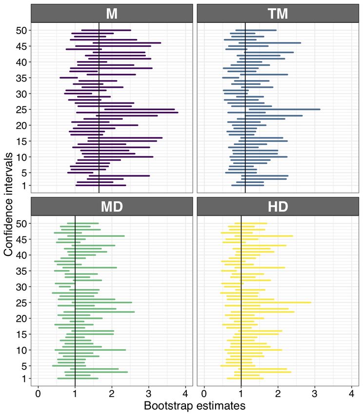
For instance, for a 95% CI, the lower bound is defined as the 2.5th quantile of the bootstrap
distribution, and the upper bound at the 97.5th quantile. Because the bootstrap distribution is an
estimate of the sampling distribution, its standard deviation provides an estimate of the standard
error, here of the mean. The bootstrap distribution is positively skewed (skewed to the right),
correctly suggesting that the sampling distribution of the mean is asymmetric. This is correct
because we draw the data from a lognormal distribution and not from a normal distribution, as
assumed by the T- distribution in Figure 1B.

The P value is computed as the minimum of the proportion of bootstrap means larger than the
null (2) and the proportion of bootstrap means smaller than the null, multiplied by two (here
bootstrap P = 0.257). Intuitively, it reflects how deeply the null value is nested within the
bootstrap distribution. When the null value is exactly in the middle of the bootstrap distribution,
the P value is 1, when it falls completely outside the distribution, the P value is 0. Finally, readers
interested in bias and its bootstrap estimation will find detailed illustrations and code in another
tutorial (Rousselet & Wilcox, 2019).

The bootstrap method described above is called the percentile bootstrap, first described in 1979
in Bradley Efron’s seminal paper (Efron, 1979). Since 1979, many other bootstrap techniques
have been developed, and we will describe only one other version in a later section: the
bootstrap-t technique (also referred to as percentile-t bootstrap), in which the bootstrap is used to
compute a data-driven T distribution under the null hypothesis. More in depth coverage of the
bootstrap and its many variants is available in several books and articles (Efron & Tibshirani,
1986, 1994; Hesterberg, 2015; Wilcox, 2017; Wilcox & Keselman, 2003). In the rest of this
tutorial, we refer to the percentile bootstrap as the bootstrap for short.

As illustrated already, the bootstrap is a data-driven (we only use the data at hand) and non-
parametric (we do not assume the data can be modelled by a distribution with a fix set of
parameters) method, and if the original sample size and the number of bootstrap samples are
large enough, the bootstrap distribution does a good job at capturing the shape of the sampling
distribution of the quantity of interest. The data-driven, non-parametric aspect means that the
bootstrap cannot suggest impossible confidence bounds, unlike standard parametric methods.
For instance, consider the percentage correct data in Figure 2. Panel A illustrates data and
                                                                                            Page 8 of 42
standard confidence intervals. Condition 1 shows a sample well spread out with a mean around
74. In condition 2, most participants are near the ceiling. In condition 3, the lowest value from
condition 2 was replaced by an outlier with a score of 60. Now the upper bound of the
confidence interval is slightly over 100%, which is of course impossible. This is because the
model used to build the confidence interval is incorrect in this case: it assumes sampling from
continuous and symmetric distributions, whereas our sample comes from a bounded and
asymmetric distribution. Unfortunately, in our experience, impossible CIs are fairly common in
publications and presentations. In contrast, the bootstrap makes no parametric assumptions
about the population our samples come from and instead uses the sample only, such that the
bootstrap confidence intervals cannot, by definition, extend beyond the smallest or largest
observations in our sample (Figure 2B).
Figure 2. Application of the bootstrap to percent correct data. Each grey disk is an observation.
The black disk marks the sample mean. The error bars mark the 95% confidence intervals, computed
using the standard T- test equation (A) or the bootstrap (B). This figure was created using the R notebook
pc.Rmd.
To illustrate that the bootstrap can provide a good approximation of sampling distributions, let’s
consider a population with a standard lognormal distribution (Figure 3). This distribution is
Page 9 of 42positively skewed and it is has a zero lower bound (only positive values can be observed), as one
could observe for instance with reaction times, fixation durations, pupil diameter, BMI etc. As
such, it provides a much better example of the sort of continuous distributions we encounter in
psychology (and in neuroscience). More generally in the social and life sciences, many quantities
have a skewed distribution similar to the one shown in Figure 3 (Limpert & Stahel, 2017;
Limpert, Stahel, & Abbt, 2001).
Figure 3. Lognormal and normal distributions. The two distributions have the same mean and
the same variance. Unlike the normal distribution, the lognormal distribution is skewed and bounded,
similarly to most quantities we measure in psychology and in neuroscience. This figure was created using
the R notebook sampdist.Rmd.
To visualise examples of sampling distributions, we take 50,000 random samples from a
lognormal distribution and each time compute some statistics (Figure 4). We could compute the
mean, but it is only one of many options to quantify the location of a distribution, and not a good
one when there is skewness because it can reflect a highly atypical response (Rousselet & Wilcox,
2019). More generally, one has to go beyond the mean to understand how distributions differ
Page 10 of 42(Rousselet et al., 2017). So here, as an example, we compute the 20% trimmed mean, which
provides a robust measure of location (Wilcox, 2017).
To compute a 20% trimmed mean, observations are sorted, the lower and upper 20% are
discarded and the remaining observations are averaged. In this context, the mean is a 0%
trimmed mean and the median is a 50% trimmed mean. In our example, we compute 50,000
trimmed means for sample sizes n=20, 30 and 50. In other words, we look at how the 20%
trimmed mean is distributed when we perform many experiments with certain sample sizes.
These sampling distributions are usually unobservable, but we can visualise them here because
we performed simulations. As shown in the top row of Figure 4, all sampling distributions are
positively skewed, even for n=50. They also get narrower with increasing sample size, because
the larger the sample, the closer on average each experimental estimate is to the population
value.
The bootstrap aims to estimate the shape of these distributions. In each column of Figure 4,
under the sampling distribution, four of the 50,000 samples are illustrated. For each sample,
5,000 bootstrap estimates are computed. In all cases, the bootstrap distributions suggest,
correctly, that the sampling distribution is positively skewed. The exact shape of each bootstrap
sampling distribution is dictated by the sample at hand, and no other information is taken into
account. Because of this, some bootstrap distributions are more skewed if the samples contain
more extreme values—for instance contrast samples 1 and 4 in column 1. With increasing
sample sizes, the bootstrap distributions also tend to be narrower, mirroring the behaviour of the
sampling distributions.
Page 11 of 42Figure 4. Bootstrap estimates of sampling distributions. The top row shows sampling
distributions of the 20% trimmed mean for sample size of n=20, n=30 and n=50. These distributions
were obtained by taking 50,000 samples from the lognormal distribution illustrated in Figure 3. The
vertical dashed lines mark the population 20% trimmed mean. In each column, the dyads of rows under
the sampling distribution show 4 of the 50,000 samples. In each dyad, the narrow panel contains a
scatterplot of the observations in the sample. The vertical black line marks the sample 20% trimmed
mean. The lower panel shows the bootstrap distribution of the 20% trimmed mean, based on 5,000
bootstrap samples. This figure was created using the R notebook sampdist.Rmd and was inspired by the
illustrations in (Hesterberg, 2015).
Figure 4 also provides an important reminder about bootstrap inferences. Each bootstrap
distribution is centred around the sample estimate, not the population value, so the bootstrap can
improve inferences, not estimation (Hesterberg, 2015). Moreover, bootstrap CIs, like any other
CIs, vary across experiments (Figure 5). Therefore, if we perform a single experiment, the CI we
obtain does or does not contain the population value we’re trying to estimate. The coverage
Page 12 of 42probability (say 95%) is only defined in the long run; there is no guarantee for a single
experiment (Greenland et al., 2016). And as we will see later, the actual coverage can be quite
different from the intended one—for instance an intended 95% CI can, in some situations, in
reality be a 90% CI.
Figure 5. 50 experiments, 50 bootstrap confidence intervals. For each experiment, a random
sample of size n=30 was taken from the lognormal distribution shown in Figure 3. For each sample,
bootstrap CIs were computed using 5,000 bootstrap samples, for four quantities: the mean (M), the 20%
trimmed mean (TM), the median (MD), and the Harrell-Davis estimate of the 50th quantile (HD). In each
panel, the vertical black line indicates the population value. This figure was created using the R notebook
coverage.Rmd.
Page 13 of 42Limitations of the bootstrap
Before we look at examples of applications of the bootstrap, it is worth clarifying two common
misconceptions. First, the bootstrap is sometimes presented as being robust, but this is not the
case. There are several statistical definitions of robustness, but loosely speaking, one important
aspect is whether one extreme value can influence the outcome of a statistical test, in particular a
confidence interval (Wilcox, 2017). Let’s look at the example in Figure 6. We consider a single
sample (n=11) in which the largest value is progressively increased. As a result, the sample mean
increases progressively, because it can be influenced by a single extreme value (Figure 6A).
Similarly, the standard T-test CI for the mean also increases, because it relies on the variance,
which is a non-robust measure of spread. If instead we use the bootstrap, the CIs are also inflated
by the extreme value (Figure 6B). However, because the bootstrap accommodates asymmetric
CIs, the effect is only seen on the side of the extreme value. So, although the bootstrap CI of the
mean is not robust, it is in this case more informative than the standard one. Finally, if we use the
bootstrap to make inferences about the median, the CIs are not affected at all by the extreme
value (Figure 6C) because the median (and not the bootstrap procedure) is a robust estimator of
location.
Figure 6. The bootstrap is not robust. Grey disks are observations. In each condition we consider a
sample of n=11 observations. The 10 lowest observations are constant across conditions and panels. The
Page 14 of 42largest observation is progressively shifted upward from condition 1 to 7. In each condition, the black disk
marks the sample estimate (mean or median), and the vertical line marks the bounds of the CI. For ease of
comparison, the horizontal dashed lines indicate the bounds of the CI in condition 1. A. Standard T-test
CI for the mean. B. Bootstrap CI for the mean. C. Bootstrap CI for the median. All bootstrap CI were
computed using 2,000 bootstrap samples. This figure was created using the R notebook notrobust.Rmd.
In sum, Figure 6 helps illustrate an important lesson: robustness comes from a conjunction of
choices—a method to build a confidence interval, and the estimator for which a confidence
interval is built. And unfortunately there is no universal solution. Depending on the types of
distributions considered, different methods offer different performances and help answer different
questions (Wilcox, 2017).
Second, the bootstrap is sometimes presented as not making any inferences about the data, unlike
standard parametric methods. Although the bootstrap does not make assumptions about the
shape of the distribution (the shape is not defined by parameters, hence the non-parametric
label), it does make very strong assumptions about the data: indeed the bootstrap assumes that
the observations in the original sample are the only ones that can ever be observed! This strong
assumption explains why the bootstrap does not work well with small sample sizes—in some
situations it gives weirdly shaped bootstrap distributions and inaccurate CIs. This is the case for
instance when making inferences about the median, as we will see in a later example. That’s
because the median, as well as most quantile estimators, do not deal well with tied values, which
tend to occur frequently in bootstrap samples derived from small original samples. Several
solutions exist: for instance to use estimators that can handle tied values, such as the Harrell-
Davis quantile estimator (Harrell & Davis, 1982), or to use a bootstrap technique that makes
parametric assumptions, such as the percentile-t technique—see description later in the tutorial.
More importantly, like any other statistical method, the bootstrap has no magical property: it is
only useful when a sufficient sample size has been collected. Which brings us to an important
question: how do we know that a method does what we expect it to do? Using simulations of
course!
Page 15 of 42Using simulations to check the behaviour of bootstrap confidence intervals
As we mentioned previously, the behaviour of confidence intervals can only be defined in the
long-run. There is no guarantee for a single experiment. This was illustrated in Figure 5, in
which 50 simulated experiments were carried out, each time drawing a sample of size n=30, and
for each sample a bootstrap CI was computed for each of four measures of central tendency: the
mean, the 20% trimmed mean, the median, and the Harrell-Davis estimator of the 50th quantile.
Each of these estimators can be used to quantify the location of the bulk of the observations,
although they behave differently depending on skewness, sample size and in the presence of
outliers (Wilcox, 2017). They also answer slightly different questions about the data: for instance,
when we use the 20% trimmed mean, we make inferences about the 20% trimmed mean of the
population, not another quantity.
In our example, across simulated experiments, it is striking to see the large changes in position
and width of the CIs: sometimes they include the population value, sometimes they don’t, and
they can be narrow or wide. This is a healthy reminder that inferences from a single experiment
should be considered with caution.
More generally, to assess CI methods, we proceed by performing simulations in tightly controlled
conditions, for which we know what the result is. For instance, in Figure 4, we sampled from the
lognormal population illustrated in Figure 3. Having defined a population of interest, we draw
random samples of a certain size, and for each sample calculate a quantity of interest (say the
median) and its confidence interval. In this approach, we can vary any aspect or parameter of the
simulation we want to investigate: the population we sample from, the size of the sample, the
quantity to estimate, the method used to build the CI, and for bootstrap methods, the number of
bootstrap samples.
Then, what do we look for? For CIs, the first concern is coverage. For a 95% CI, we need to
ensure that in the long-run, 95% of such CIs do contain the population value we try to estimate.
For instance, Figure 7A shows the results of a simulation in which in each iteration, we took a
sample of size n=10 and computed bootstrap CIs for the same four measures of central tendency
we used in Figure 5. We varied the number of bootstrap samples from 500 to 10,000, in steps of
Page 16 of 42500. The results confirm the observations we made in Figure 6: bootstrap CIs of the mean do not
perform well, with coverage near 80%. Increasing sample size to n=30 improves matters, but still
leads to coverage of about 89%, instead of the expected 95% (Figure 7B). So using the mean in
conjunction with the bootstrap is clearly not recommended. Other measures of central tendency
are associated with CI coverage much closer to the nominal level.
Figure 7. Confidence interval coverage. Results of simulations in which we sampled from the
standard lognormal distribution illustrated in Figure 3. For each sample, bootstrap CIs were computed for
four quantities: the mean (M), the 20% trimmed mean (TM), the median (MD), and the Harrell-Davis
estimate of the 50th quantile (HD). For each combination of sample size and number of bootstrap
samples, coverage was computed as the proportion of simulations in which the CI included the population
value. The number of iterations per simulation was 5,000 for panels A, B and D, and 10,000 for panel C.
nboot = number of bootstrap samples. This figure was created using the R notebook coverage.Rmd.
Page 17 of 42Instead of varying the number of bootstrap samples, we could also choose a fix number, and vary
the sample size. Whether we used 200 or 2000 bootstrap samples, the main determinant of
coverage was sample size (Figure 7C-D). Again bootstrap CIs for the mean performed poorly.
The results from Figure 7 suggest that the number of bootstrap samples does not affect the
coverage of the CIs. However, this result cannot be generalised to all situations. And the number
of bootstrap samples affects other aspects of the results, such as the precision of the bootstrap P
values and the width of the CIs (see extra figures in the notebook coverage.Rmd) . For instance,
given two methods with appropriate coverage, the one that tends to give shorter CIs seems
preferable, as it reduces our uncertainty about the population value in the long-run. So there are
various ways to decide on the number of bootstrap samples to use, and not surprisingly, there is a
whole statistical literature on the topic (Davidson & MacKinnon, 2000; Hesterberg, 2015; Olive,
2014 chap. 9; Racine & MacKinnon, 2007, 2007). In our experience, using 1,000 bootstrap
samples appears to be sufficient if the goal is to have coverage at the nominal level. For statistical
power, there might be situations where more samples are required. Given the speed of modern
computers, for relatively simple applications there is no reason not to use 5,000 or even 10,000
bootstrap samples—except extra time and energy consumption, there is no negative effect of
using more samples.
The choice of the number of bootstrap samples for a particular type of data and analysis is best
made using simulations, as demonstrated in Figure 7 for instance. Another approach is to run the
same bootstrap analysis a few times: the results should not change much across analyses of the
same data. One particular aspect of the results to consider is the stability of the CI bounds. Let
say we perform one experiment and obtain the sample in Figure 8A. We could then compute CIs
for different measures of central tendency (Figure 8B). But what happens if we compute a
bootstrap CI several times using the same data? Because of random sampling, the results differ
slightly across CIs (Figure 8C). And this variability decreases with the number of bootstrap
samples (Figure 8D). In this example, there is also more variability for the higher bound of the CI
than the lower bound, which is explained by the skewness of the original sample. So the number
of bootstrap samples should also be chosen based on the level of precision desired and the context
in which the results are interpreted (Hesterberg, 2015). To obtain stable CI bounds, Hesterberg
Page 18 of 42(2015) recommends at least 10,000 in routine applications, and much more when the outcome of
the test is used to make strong decisions. For complex applications, for instance brain imaging
analyses, such choices could lead to extra minutes, hours and sometimes days of calculations, but
this extra time remains short relative to the time spent acquiring the data.
Page 19 of 42Figure 8. Performance diagnostics: stability. A. One sample (n=30) from a standard lognormal
distribution. B. Four bootstrap sampling distributions and CIs computed using 5,000 bootstrap samples,
for four quantities: the mean (M), the 20% trimmed mean (TM), the median (MD), and the Harrell-Davis
estimate of the 50th quantile (HD). C. Twenty bootstrap CIs for the same sample illustrated in panel A.
500 bootstrap samples were used to compute each CI. D. Variability of the CI bounds, measured as the
Page 20 of 42standard deviation across 2,000 CI bounds, as a function of the number of bootstrap samples. This figure
was created using the R notebook coverage.Rmd.
Group comparisons
The examples covered so far used one-sample CIs. We now turn to the topic of group
comparisons. Similarly to the one-sample case, the bootstrap for group comparisons follows the
logic of the data acquisition process. For two independent groups, we sample observations with
replacement independently from each group. If group 1 has n1 observations, we sample n1
observations with replacement. Similarly, in group 2 we sample n2 observations with
replacement. If the groups differ in sample size, we preserve this size difference in our bootstrap
samples.
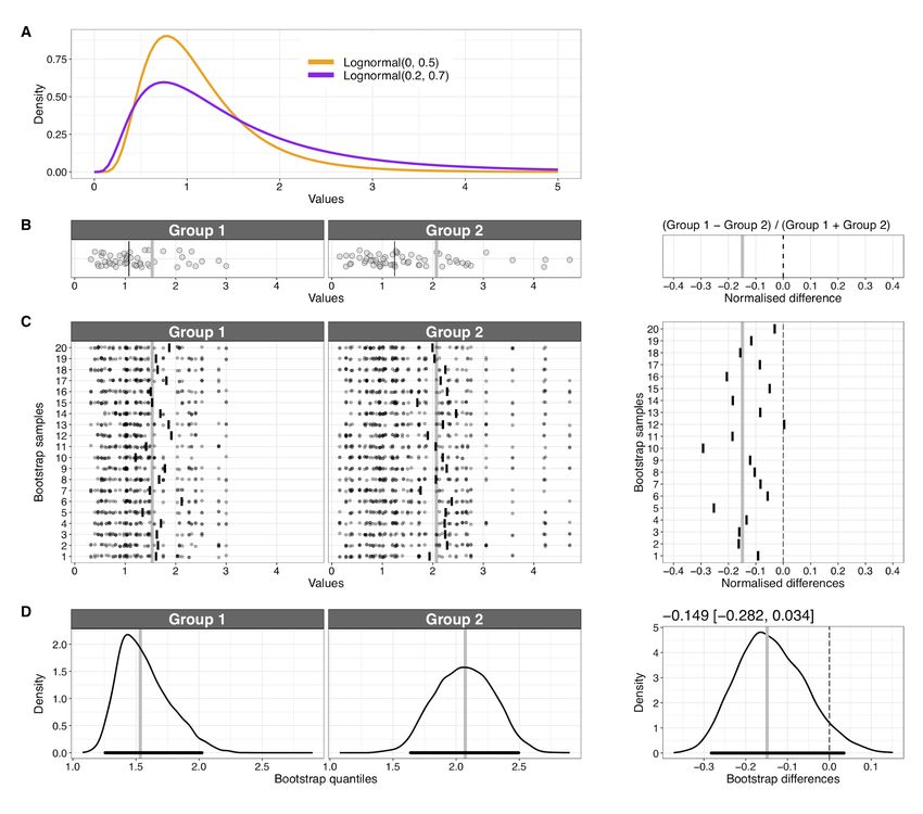
Now let say we conducted an experiment and collected observations from two groups, each from
a different population (Figure 9A & B). Because of previous research, we suspect that the groups
might differ in their right tails (more extreme observations). So instead of the traditional measures
of central tendency, like the mean or the median, here we estimate the 3rd quartile of the
marginal distributions. Then we use the bootstrap to derive a CI for the 3rd quartile of each
group, as well as for the difference between groups. Twenty bootstrap samples are illustrated in
Figure 9C. For each bootstrap sample, we compute the difference between the two bootstrap
estimates; or some other quantity of interest: it could be some transformation of the difference,
the ratio between groups, etc. Here, to illustrate that with the bootstrap we can build confidence
intervals for any quantity, the group estimation is performed on a normalised difference of
quartiles, defined as (q3gp1- q3g p2) / (q3gp1+ q3gp2) , thus accounting for the total magnitude.
The CI for the normalised difference is compatible with a value of zero, but also more negative
values. The CI actually contains the population normalised difference (-0.17), but many more
trials would be required to get a narrower CI that excludes zero. For instance, with a random
sample of 200 observations for each group we obtained a CI of [-0.23, -0.10]. Of course, one
could perform a simulation in which sample size is varied systematically, to determine the
number of observations needed to detect or precisely estimate the effect.
Page 21 of 42Figure 9. Comparison of two independent groups. A. Two populations that differ in skewness. B.
Two independent samples, one from each population. Group 1 contains n=50 observations (left panel);
group 2 contains n=60 observations (middle panel). The thick vertical grey line marks the 3rd quartile; the
thin vertical black line marks the 2nd quartile (median). In the right panel, the thick vertical grey line
marks the sample normalised group difference between 3rd quartiles, whereas the thin vertical black
dashed line is a zero reference line. The same lines appear in subsequent panels. C. Examples of
bootstrap samples. Each disk is a bootstrap observation. For each bootstrap sample the short vertical black
line indicates the bootstrap 3rd quartile (left and middle panels), or the normalised difference (right panel).
D. Bootstrap distributions of 3rd quartiles for the two groups (left and middle panels) and of the
normalised quartile difference (right panel). The thick horizontal black lines indicate 95% bootstrap CIs.
This figure was created using the R notebook 2indgps.Rmd.
Page 22 of 42Correlations
In addition to group comparisons, another common topic in psychology is to make inferences
about correlations. To compute bootstrap CI for correlations, the basic recipe is to sample pairs
of observations with replacement. Again, we follow the data acquisition process: if different
measurements were made in the same participants, then participants should be sampled with
replacement, keeping all their measurements together. The same strategy applies to regression
coefficients. Correlation and linear regression are huge topics, so we only address basic principles
here (Wilcox, 2017). In general, for robust estimators, the bootstrap performs well, meaning that
CIs with the expected coverage are obtained. In contrast, Pearson’s correlation and the standard
ordinary least square (OLS) regression are problematic for a number of reasons. Satisfactory
bootstrap CIs can nevertheless be obtained with a simple adjustment to the way the quantiles of
the bootstrap distributions are computed—see details in (Wilcox, 2009, 2017). However,
estimators robust to univariate, or even better multivariate, outliers should be preferred to these
standard yet outdated methods (e.g. Pernet, Wilcox, & Rousselet, 2013).
Figure 10 presents an application of the bootstrap method to correlation analyses. Two
measurements were made in two independent groups of participants (both n=50). Dependent
cases are covered in the notebook compcorr.Rmd—see also Wilcox (2016, 2017). Group 1 was
sampled from a population with correlation 0.5, group 2 from a population with correlation 0.6.
We use Spearman’s correlation, which is robust to univariate outliers (Pernet et al., 2013). We
compute a bootstrap CI for each correlation by sampling pairs of observations with replacement.
In our experience, very often two correlations are presented side-by-side, with the implicit
assumption that if one is significant according to some arbitrary P value threshold, and the other
is not, then the two correlations differ. This is however a classic interaction fallacy, akin to
looking at the simple effects in an ANOVA, without testing the interaction (Gelman & Stern,
2006; Nieuwenhuis, Forstmann, & Wagenmakers, 2011). So an explicit comparison of
correlation coefficients is needed. Unfortunately, the popular comparison of correlation
coefficients using Fisher’s z transform is inappropriate because it is not robust to deviation from
normality (Duncan & Layard, 1973). In contrast, the comparison of two correlation coefficients is
Page 23 of 42straightforward with the bootstrap. To compare two independent correlation coefficients using
the bootstrap, we proceed like this:
- sample participants with replacement, independently in each group (concretely, for 2
groups, we sample dyiads of observations, preserving the dependency among
observations);
- compute the two correlation coefficients based on the bootstrap samples;
- save the difference between correlations;
- execute the previous steps many times;
- use the distribution of bootstrap differences to derive a confidence interval.
Page 24 of 42Figure 10. Bootstrap correlation analysis. A. Independent correlations, one in each of two groups.
Sample size is n=50 in each group. Data from group 1 are from a population with correlation 0.5. Data
from group 2 are from a population with correlation 0.6. The panel on the right reports the Spearman’s
correlation coefficient for each group and their difference. B. Examples of three bootstrap samples, one
for each group, with the respective correlation coefficients in the right column. Darker disks represent
Page 25 of 42observations sampled more than once. C. Bootstrap sampling distributions of the correlation coefficients
and their differences, based on 5,000 bootstrap samples. The vertical lines mark the sample coefficients.
The larger variability in group 1 leads to a broader bootstrap distribution. The thick horizontal black lines
indicate 95% bootstrap CIs. This figure was created using the R notebook compcorr.Rmd.
Based on 5,000 bootstrap samples, the bootstrap CI for the difference between Spearman’s
correlation coefficients suggests considerable uncertainty [-0.386, 0.194], which is compatible
with a population correlation difference of zero, as well as many positive and predominantly
negative values. Larger sample sizes would be needed to detect or precisely estimate the
population difference. Based on a simulations with 5,000 iterations, 599 bootstrap samples and
assuming normal distributions and a population difference of 0.1 (correlation of 0.5 in group 1
and 0.6 in group 2), for 50% of correct detection in the long run (true positives, or power), we
need at least 459 observations in each group. For 70% correct detection, we need at least 717
observations in each group! If the goal is to estimate the population difference precisely, how
many trials do we need? For 50% of experiments to be within +/- 0.05 of the true correlation
value, we need at least 200 observations in each group. For 70% of experiments to be within +/-
0.05 of the true correlation value, we need at least 479 observations in each group. Thus, to
successfully detect or estimate correlation differences between independent groups requires a lot
more observations than is typically used in psychology experiments.
Extension to other designs
The bootstrap can be extended beyond the simple comparisons of two groups we have covered
so far: examples include multiple linear contrasts and various types of ANOVA designs, including
ANCOVAs (Wilcox, 2017). Here we look at an application of the bootstrap to a hierarchical
dataset. Imagine we collected reaction times from 20 participants in a lexical decision task, with
200 trials per condition (Word and Non-Word conditions, Figure 11). This example dataset was
subsampled from a much larger dataset (Ferrand et al., 2010). The structure of the data is
hierarchical because trials are nested within participants. There are many ways to analyse such
data, but a substandard yet typical approach is to ignore the variability across trials by
Page 26 of 42summarising the distribution for each participant and each condition using a single value
(Rousselet & Wilcox, 2019). For instance, we could summarise each of the 40 distributions in
Figure 11A using the 20% trimmed mean; we’re then left with 20 values per condition and their
differences (Non-Word minus Word, Figure 11B). In turn, we summarise the distributions across
participants, for each condition and their difference: for simplicity here, we use again the 20%
trimmed mean. Finally, we use the bootstrap to compute CIs for the group trimmed means in
each condition, and their difference (Figure 11C). To apply the standard bootstrap, we proceed
as we did for the correlations: we sample participants with replacement, that is pairs of trimmed
means, one in each condition. This approach ignores, however, the variability across trials.
A hierarchical bootstrap can be used to exploit within and between subject variability. There are
several approaches to implement a hierarchical bootstrap (Roberts & Fan, 2004). One approach
is to follow the data acquisition process by resampling first at the highest level (participants), then
at the next level (trials). This is also called a nested bootstrap, because the trials are nested within
participants. In each bootstrap sample, we sample participants with replacement; then for each
participant, we sample trials with replacement, independently for each condition. The 20%
trimmed mean is computed for each condition across trials, and the results from the two
conditions subtracted (Non-Word minus Word). Then, the 20% trimmed mean is computed
across participants for each condition and their difference. In our example, the bootstrap
sampling distributions and the CIs from the hierarchical procedure are very similar to the
standard bootstrap ones. However, this is not always the case. In particular, the hierarchical
procedure can make substantial improvements when making inferences about quantiles or the
median for small sample sizes. For instance, in Figure 11D, the bootstrap sampling distributions
for the median are very irregular when using the standard bootstrap (sampling at the participant
level only). This is because for small sample sizes, bootstrap samples tend to contain too many
tied values, such that the bootstrap median takes only a few discrete values. With the nested
bootstrap, sampling trials with replacement adds variability to the values from each participant,
which ultimately leads to smoother bootstrap distributions and, in this example, slightly different
CIs.
Page 27 of 42Figure 11. Hierarchical bootstrap. A. Distributions of 200 reaction times in the Word and Non-
Word conditions for 20 participants. B. Distributions of 20% trimmed means across trials for the Word
and Non-Word conditions and their differences. In each panel, there is a disk for each of the 20
participants. The vertical black lines mark the 20% trimmed means across participants in each condition
and the difference. C. Bootstrap distributions of 20% trimmed means across participants, based on 5,000
Page 28 of 42bootstrap samples. The thick horizontal lines indicate 95% bootstrap CIs. Orange = bootstrap at the
participant level only, black = hierarchical bootstrap of participants and their nested trials. D.
Distributions of participants’ median reaction times in the two conditions and their differences. The
vertical black lines mark the medians across participants. E. Bootstrap distributions of group medians.
This figure was created using the R notebook 2depgps.Rmd.
Bootstrap-t technique
Before we conclude, in this last section we introduce an alternative to the standard (percentile)
bootstrap presented so far. As mentioned in the introduction, there are many variants of the
bootstrap, but in psychology, two methods cover most of the applications: the standard bootstrap
and the bootstrap-t technique—also known as the percentile-t bootstrap or the studentized
bootstrap (Efron & Tibshirani, 1994; Wilcox, 2017). As we saw in previous examples, for
inferences on the population mean, the standard T- test and the bootstrap can give unsatisfactory
results when sampling from skewed distributions, especially when sample size is small. To
illustrate the problem with the t-test, imagine that we sample from populations of increasing
skewness (Figure 12A). Here we use the so-called g & h distributions, in which parameter g
controls the skewness, and parameter h controls the thickness of the tails—a normal distribution
is obtained by setting g=h=0 (Hoaglin, 1985). If we take many samples of size n=30 from these
distributions, and for each sample we compute a T value, using the population mean as the null
value, we obtain progressively more negatively skewed T value sampling distributions (Figure
12B). However, when we perform a T-test, the T values are assumed to be symmetric,
irrespective of sample size. This assumption leads to incorrect CIs. The idea behind the
bootstrap-t technique is to use the bootstrap to compute a data-driven T distribution. In the
presence of skewness, this T distribution could be skewed, as suggested by the data. Then, the
appropriate quantile of the bootstrap T distribution is plugged into the standard CI equation to
obtain a parametric bootstrap CI.
Page 29 of 42Figure 12. Bootstrap-t technique. A. Probability density functions for g & h distributions. Parameter
g varies from 0 to 1. Parameter h=0. B. Sampling distribution of T values for the different g values. Results
are based on a simulation with 50,000 iterations and samples of size n=30. C. Comparison of T
distributions for g=1: theoretical T is the one used in the T- test (red), empirical T is from panel B (black).
The red and black vertical lines indicate the T quantiles for a 95% CI. The grey lines show examples of
20 bootstrap sampling distributions, based on samples of size n=30 and 599 bootstrap samples. D-I.
Results of a simulation with 20,000 iterations, sample sizes of n=30, and 599 bootstrap samples. Panels D
and E show results for the mean, panels F and G for the 10% trimmed mean, and panels H and I for the
20% trimmed mean. This figure was created using the R notebook ptb.Rmd.
Figure 13 illustrates the procedure for a CI for the population mean (row A) and for the
population 20% trimmed mean (row B). In both cases, we start with the same sample of 30
observations from a g & h distribution with g=1 and h= 0. In a first step, we centre the
distribution: for inferences on the mean, we subtract the mean from each observation in the
sample, so that the mean of the centred distribution is now zero. This is a way to create a data-
Page 30 of 42driven null distribution, in which there is no effect (the mean is zero), but the shape of the
distribution and the absolute distance among observations are unaffected, as shown in the second
column. For inferences on the 20% trimmed mean, we subtract the 20% trimmed mean from
each observation, so that the centred distribution now has a 20% trimmed mean of zero. In the
next step, we sample with replacement from the centred distribution many times, and for each
random sample we compute a T value. That way, we obtain a bootstrap distribution of T values
expected by random sampling, under the hypothesis that the population has a mean (or 20%
trimmed mean) of zero, given the distribution of the data. Then, we use some quantile of the
bootstrap T distribution in the standard CI equation. Because the bootstrap distribution is
potentially asymmetric, we have two choices of quantiles: for a 95% CI, either we use the 0.025
and the 0.975 quantiles of the signed T values to obtain a potentially asymmetric CI, also called
an equal-tailed CI, or we use the 0.95 quantile of the absolute T values, thus leading to a
symmetric CI. In our example, for the mean the symmetric CI is [-0.4, 1.62] and the asymmetric
CI is [0.08, 1.87]; for the 20% trimmed mean the symmetric CI is [-0.36, 0.59] and the
asymmetric CI is [-0.3, 0.67]. So the choice of method can have a substantial impact on the CI.
In general, when comparing 20% trimmed means, there are indications that an asymmetric
confidence interval is a bit better than a symmetric confidence interval. When comparing means,
there are theoretical results suggesting that a symmetric confidence interval is preferable, but this
issue is in need of further study (Wilcox, 2017).
Page 31 of 42Figure 13. Bootstrap-t technique explained. A. Inferences on the population mean. The first panel
illustrates a sample of size n=30 from a g & h distribution with g= 1 and h=0. The same sample is used in
rows A and B. The horizontal line indicates the sample mean. In the second panel, the distribution has
been mean centred, so that the sample mean is now zero. The third panel shows 5,000 bootstrap T values
obtained by sampling with replacement from the mean centred data. In the asymmetric bootstrap-t
technique, the quantiles (red vertical lines) of that distribution of T values are used to define the CI
bounds. The insets contain the formulas for the lower (CIlo) and upper bounds (CIup) of the CI. Note that
the lower T quantile is used to compute the upper bound (this not an error). In the symmetric bootstrap-t
technique, one quantile of the distribution of absolute T values is used to define the CI bounds. B. Same
as A, but for inferences on the population 20% trimmed mean. This figure was created using the R
notebook ptb.Rmd.
Why does this approach work better than the standard T- test CI? Imagine we take multiple
samples of size n=30 from a g & h distribution with g= 1 and h=0 (Figure 12C). The standard T-
test assumes the sampling distribution in red, symmetric around zero. From our simulation in
Figure 12B, we know that the sampling distribution is actually asymmetric, with negative
skewness, as shown in black. However, the black empirical distribution is unobservable, unless we
can perform thousands of experiments. So, with the bootstrap, we try to estimate this correct, yet
unobservable, sampling distribution. The grey curves in Figure 12C show examples of 20
simulated experiments: in each experiment, a sample of 30 observations is drawn, and then 5,000
bootstrap T values are computed. The resulting bootstrap sampling distributions are negatively
Page 32 of 42skewed and are much closer to the empirical distribution in black than the theoretical symmetric
distribution in red. Thus, it seems that using data-driven T distributions could help achieve better
CIs than if we assumed symmetry.
How do these different methods perform? To find out we carry out simulations in which we draw
samples from g&h distributions with the g parameter varying from 0 to 1, keeping h = 0. For each
sample, we compute a one-sample CI using the standard T- test, the two bootstrap-t methods just
described, and the percentile bootstrap. When estimating the population mean, for all four
methods, coverage goes down with skewness (Figure 12D). Among the parametric methods, the
standard T- test is the most affected by skewness, with coverage less than 90% for the most
skewed condition. The asymmetric bootstrap-t CI seems to perform the best. The percentile
bootstrap performs the worst in all situations, and has coverage systematically below 95%,
including for normal distributions.
In addition to coverage, it is useful to consider the width of the CIs from the different techniques
(Figure 12E, G, I). The width of a CI is its upper bound minus its lower bound. For each
combination of parameters. the results are summarised by the median width across simulations.
At low levels of asymmetry, for which the three parametric methods have roughly 95% coverage,
the CIs also tend to be of similar widths. As asymmetry increases, all methods tend to produce
larger CIs, but the T- test produces CIs that are too short, a problem that stems from the
symmetric theoretical T distribution, which assumes T values too small. Compared to the
parametric approaches, the percentile bootstrap produces the shortest CIs for all g values.
The low coverage observed in the previous simulations can be addressed by making inferences
about trimmed means instead of the mean, which requires several adjustments to the T-test
equation (Tukey & McLaughlin, 1963). With the 10% trimmed mean, coverage improves for all
methods, with values now close to the nominal level even for the most skewed distributions,
though the T- test performs less well than all three bootstrap techniques (Figure 12H). CIs are
also overall shorter for all methods compared to CIs on the mean (Figure 12I). The results were
similar when making inferences about the 10% trimmed mean (Figure 12F-G). Also, the shorter
CIs obtained with the percentile bootstrap compared to the bootstrap-t CIs, for similar coverage,
suggest it could beneficial to use the percentile bootstrap in conjunction with trimmed means.
Page 33 of 42More generally, inferences about trimmed means are robust to outliers, which can have
devastating effects on the power of methods using the mean (Wilcox, 2017; Wilcox & Rousselet,
2018). Finally, based on simulations, it seems that to make inferences about the mean or when
trimming less than 20%, the bootstrap-t technique performs well in many situations and should
be prefered over the percentile bootstrap; when trimming at least 20%, the standard bootstrap
approach is recommended (Wilcox, 2017).
Conclusion
In this tutorial, we introduced the bootstrap, its core mechanism, sampling with replacement, its
main output, a bootstrap sampling distribution, and presented its strengths and weaknesses. The
bootstrap is a very versatile approach to statistical inferences, but it is by no means a magical
recipe. It can perform poorly in some situations, for instance when making inferences about
means, or about medians for relatively small samples. But combined with robust estimators, the
bootstrap often outperforms other approaches, and can provide a simple solution to compute CIs
when analytical solutions do not exist: this is for instance the case when making inferences about
certain quantile estimators, robust correlation and regression estimates, as well as other robust
estimators not mentioned here (Wilcox, 2017). The bootstrap-t can be used to make inferences
about means and trimmed means, and the approach can be extended to various ANOVA
designs, improving statistical power in many situations relative to standard ANOVAs on means
(Field & Wilcox, 2017).
Thus, by learning the bootstrap, users do not only get a new powerful technique in their toolbox,
but a whole set of techniques that can be applied to a large range of problems. The application of
bootstrap techniques can bring potentially more informative answers relative to standard
parametric approaches in psychology, which typically focus on mean only and are often
inappropriate. For instance, reaction time distributions contain a lot of information that is
thrown away by summarising them using the mean. The bootstrap, combined with quantile
estimation, can help provide a much more detailed understanding of how such continuous
distributions differ across conditions (Rousselet et al., 2017; Rousselet & Wilcox, 2019).
Page 34 of 42You can also read