SENSORLESS FIELD ORIENTED CONTROL WITH EMBEDDED POWER SOC - INFINEON ...
←
→
Page content transcription
If your browser does not render page correctly, please read the page content below
Sensorless Field Oriented Control with Embedded
Power SoC
Z8F68474109

Scope and purpose of this document

Figure 1
This document is meant to give the reader a basic introduction to field oriented control and how it can be
implemented on the Infineon embedded Power SoC devices for low-to-mid power 3-phase motors in
automotive applications. It is expected that the reader is familiar with the principles of motor control and its
implementation on a microcontroller based system.
The full functionality and characteristics of the embedded power devices is specified in the respective
datasheet and user’s manual. Please refer to these documents for detailed description. The TLE9879 EvalKit
has been used as hardware platform for the presented measurements, This EvalKit’s schematic and PCB layout
are the optimal starting point for developing new motor control ECUs. Similarly, the associated software project
for the FOC implementation is meant as a demonstration platform.

Note:         The following information is given as a hint for the implementation of the system only and shall not be
              regarded as a description or warranty of a certain functionality, condition or quality of the referred
              devices or presented software example.

Application Note               Please read the Important Notice and Warnings at the end of this document      Rev 1.0
www.infineon.com                                                                                           2020-03-09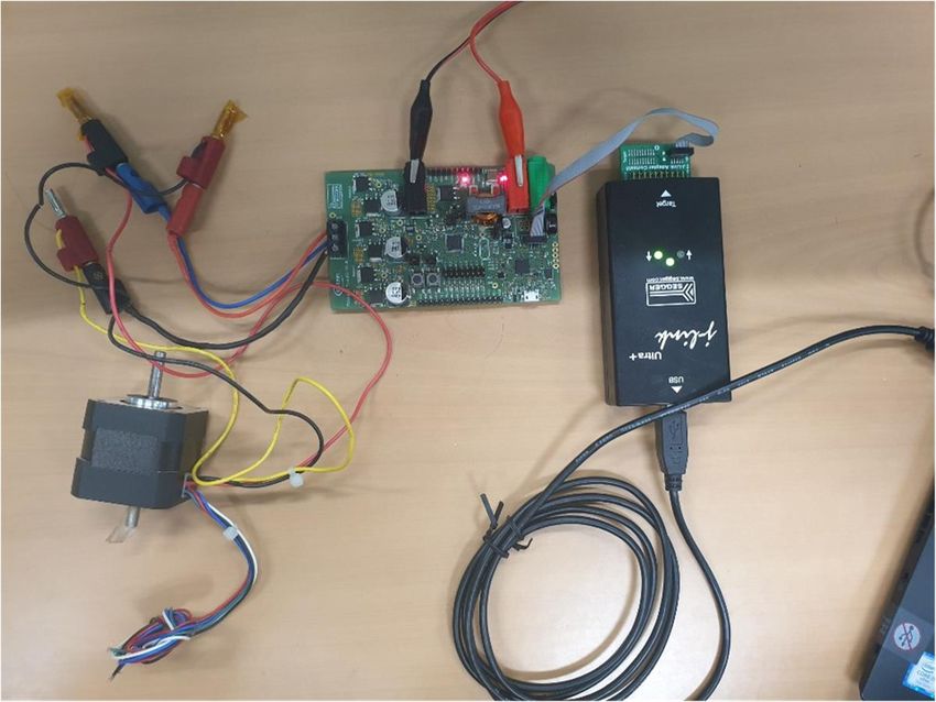
Sensorless Field Oriented Control with Embedded Power SoC
Z8F68474109

Terms and abbreviations

Terms and abbreviations
Table 1            Terms used in this document
Abbreviation                       Meaning
AC                                 Alternating Current
ADC                                Analog to Digital Converter
BLDC                               Brushless DC motor
BOM                                Bill of Materials
CPU                                Central Processing Unit
DC                                 Direct Current
ECU                                Electronic Control Unit
BEMF                               Back Electro Motive Force
EMC                                Electromagnetic Compatibility
FOC                                Field Oriented Control
MCU                                Microcontroller
NVM                                Non-volatile Memory
PMSM                               Permanent Magnet Synchronous Motor
PWM                                Pulse Width Modulation
SDK                                Software Development Kit
SoC                                System-on-Chip

Application Note                                       2                   Rev 1.0
                                                                        2020-03-09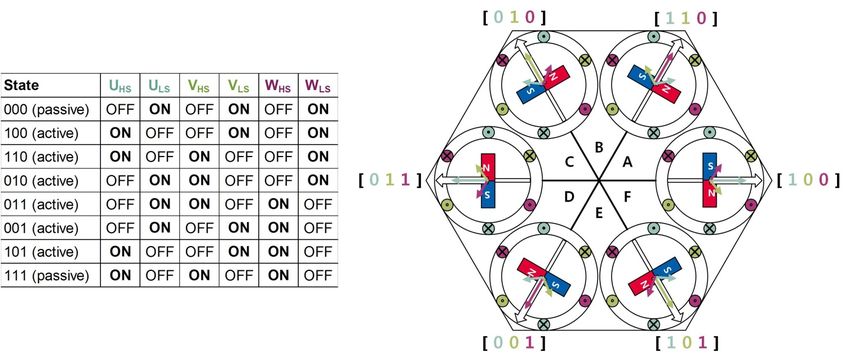
Sensorless Field Oriented Control with Embedded Power SoC
Z8F68474109

Table of contents

Table of contents

                   Scope and purpose of this document . . . . . . . . . . . . . . . . . . . . . . . . . . . . . . . . . . . . . . . . . . . . . . . . . . . . 1
                   Terms and abbreviations . . . . . . . . . . . . . . . . . . . . . . . . . . . . . . . . . . . . . . . . . . . . . . . . . . . . . . . . . . . . . . . .2
                   Table of contents . . . . . . . . . . . . . . . . . . . . . . . . . . . . . . . . . . . . . . . . . . . . . . . . . . . . . . . . . . . . . . . . . . . . . . . 3
1                  Introduction . . . . . . . . . . . . . . . . . . . . . . . . . . . . . . . . . . . . . . . . . . . . . . . . . . . . . . . . . . . . . . . . . . . . . . . . . . . 5
2                  Theory of Sensorless Field Oriented Control . . . . . . . . . . . . . . . . . . . . . . . . . . . . . . . . . . . . . . . . . . . . . 6
2.1                2-Phase (DC) Motor Basics . . . . . . . . . . . . . . . . . . . . . . . . . . . . . . . . . . . . . . . . . . . . . . . . . . . . . . . . . . . . . . . . 6
2.1.1                2-Phase Motor Control: Open Loop Voltage Control . . . . . . . . . . . . . . . . . . . . . . . . . . . . . . . . . . . . . . . 7
2.1.2                2-Phase Motor Control: Closed Loop Torque Control . . . . . . . . . . . . . . . . . . . . . . . . . . . . . . . . . . . . . . .7
2.1.3                2-Phase Motor Control: Closed Loop Speed and Torque Control . . . . . . . . . . . . . . . . . . . . . . . . . . . . 8
2.1.4                List of Equations . . . . . . . . . . . . . . . . . . . . . . . . . . . . . . . . . . . . . . . . . . . . . . . . . . . . . . . . . . . . . . . . . . . . . . . 9
2.2                3-Phase Motor Basics . . . . . . . . . . . . . . . . . . . . . . . . . . . . . . . . . . . . . . . . . . . . . . . . . . . . . . . . . . . . . . . . . . . 10
2.3                Space Vector Modulation . . . . . . . . . . . . . . . . . . . . . . . . . . . . . . . . . . . . . . . . . . . . . . . . . . . . . . . . . . . . . . . . 11
2.4                Phase Current Measurement . . . . . . . . . . . . . . . . . . . . . . . . . . . . . . . . . . . . . . . . . . . . . . . . . . . . . . . . . . . . 15
2.4.1                Limitations of Phase Current Reconstruction . . . . . . . . . . . . . . . . . . . . . . . . . . . . . . . . . . . . . . . . . . . . 17
2.5                FOC Calculations . . . . . . . . . . . . . . . . . . . . . . . . . . . . . . . . . . . . . . . . . . . . . . . . . . . . . . . . . . . . . . . . . . . . . . . 18
2.5.1                Stationary and Rotating Reference Frames . . . . . . . . . . . . . . . . . . . . . . . . . . . . . . . . . . . . . . . . . . . . . . 18
2.5.2                Sensorless FOC . . . . . . . . . . . . . . . . . . . . . . . . . . . . . . . . . . . . . . . . . . . . . . . . . . . . . . . . . . . . . . . . . . . . . . . 20
3                  Implementation of Sensorless FOC with the TLE9879 Embedded Power SoC . . . . . . . . . . . . . . 22
3.1                System overview . . . . . . . . . . . . . . . . . . . . . . . . . . . . . . . . . . . . . . . . . . . . . . . . . . . . . . . . . . . . . . . . . . . . . . . 22
3.2                Hardware components of TLE9879 . . . . . . . . . . . . . . . . . . . . . . . . . . . . . . . . . . . . . . . . . . . . . . . . . . . . . . . 22
3.2.1                ADC . . . . . . . . . . . . . . . . . . . . . . . . . . . . . . . . . . . . . . . . . . . . . . . . . . . . . . . . . . . . . . . . . . . . . . . . . . . . . . . . . 23
3.2.2                GPT12E . . . . . . . . . . . . . . . . . . . . . . . . . . . . . . . . . . . . . . . . . . . . . . . . . . . . . . . . . . . . . . . . . . . . . . . . . . . . . . 23
3.2.3                CCU6 . . . . . . . . . . . . . . . . . . . . . . . . . . . . . . . . . . . . . . . . . . . . . . . . . . . . . . . . . . . . . . . . . . . . . . . . . . . . . . . . 24
3.2.4                BDRV . . . . . . . . . . . . . . . . . . . . . . . . . . . . . . . . . . . . . . . . . . . . . . . . . . . . . . . . . . . . . . . . . . . . . . . . . . . . . . . . 25
3.2.5                Shunt Resistor & CSA . . . . . . . . . . . . . . . . . . . . . . . . . . . . . . . . . . . . . . . . . . . . . . . . . . . . . . . . . . . . . . . . . . 25
4                  Software Block Diagram . . . . . . . . . . . . . . . . . . . . . . . . . . . . . . . . . . . . . . . . . . . . . . . . . . . . . . . . . . . . . . . 26
4.1                Phase current measurement and reconstruction . . . . . . . . . . . . . . . . . . . . . . . . . . . . . . . . . . . . . . . . . . 27
4.2                Clarke Transform . . . . . . . . . . . . . . . . . . . . . . . . . . . . . . . . . . . . . . . . . . . . . . . . . . . . . . . . . . . . . . . . . . . . . . . 30
4.3                Park Transform . . . . . . . . . . . . . . . . . . . . . . . . . . . . . . . . . . . . . . . . . . . . . . . . . . . . . . . . . . . . . . . . . . . . . . . . .31
4.4                Polar to Cartesian Transform . . . . . . . . . . . . . . . . . . . . . . . . . . . . . . . . . . . . . . . . . . . . . . . . . . . . . . . . . . . . 32
4.5                Flux Estimator . . . . . . . . . . . . . . . . . . . . . . . . . . . . . . . . . . . . . . . . . . . . . . . . . . . . . . . . . . . . . . . . . . . . . . . . . 33
4.6                Angle PLL Observer . . . . . . . . . . . . . . . . . . . . . . . . . . . . . . . . . . . . . . . . . . . . . . . . . . . . . . . . . . . . . . . . . . . . . 34
4.7                PI Controller . . . . . . . . . . . . . . . . . . . . . . . . . . . . . . . . . . . . . . . . . . . . . . . . . . . . . . . . . . . . . . . . . . . . . . . . . . . 36
4.8                Cartesian to Polar Transform . . . . . . . . . . . . . . . . . . . . . . . . . . . . . . . . . . . . . . . . . . . . . . . . . . . . . . . . . . . . 37
4.9                SVM (Space Vector Modulation) . . . . . . . . . . . . . . . . . . . . . . . . . . . . . . . . . . . . . . . . . . . . . . . . . . . . . . . . . . 38
5                  Example Software . . . . . . . . . . . . . . . . . . . . . . . . . . . . . . . . . . . . . . . . . . . . . . . . . . . . . . . . . . . . . . . . . . . . . 40
5.1                Tool chain . . . . . . . . . . . . . . . . . . . . . . . . . . . . . . . . . . . . . . . . . . . . . . . . . . . . . . . . . . . . . . . . . . . . . . . . . . . . . 40

Application Note                                                                          3                                                                                     Rev 1.0
                                                                                                                                                                             2020-03-09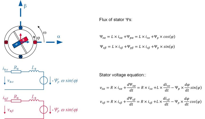
Sensorless Field Oriented Control with Embedded Power SoC
Z8F68474109

Table of contents

5.1.1                Compiler suite . . . . . . . . . . . . . . . . . . . . . . . . . . . . . . . . . . . . . . . . . . . . . . . . . . . . . . . . . . . . . . . . . . . . . . . .40
5.1.2                Debugger . . . . . . . . . . . . . . . . . . . . . . . . . . . . . . . . . . . . . . . . . . . . . . . . . . . . . . . . . . . . . . . . . . . . . . . . . . . . 40
5.1.3                SDK . . . . . . . . . . . . . . . . . . . . . . . . . . . . . . . . . . . . . . . . . . . . . . . . . . . . . . . . . . . . . . . . . . . . . . . . . . . . . . . . . 40
5.1.4                ConfigWizard . . . . . . . . . . . . . . . . . . . . . . . . . . . . . . . . . . . . . . . . . . . . . . . . . . . . . . . . . . . . . . . . . . . . . . . . . 40
5.2                Example code & project layers . . . . . . . . . . . . . . . . . . . . . . . . . . . . . . . . . . . . . . . . . . . . . . . . . . . . . . . . . . . 41
5.2.1                “App” . . . . . . . . . . . . . . . . . . . . . . . . . . . . . . . . . . . . . . . . . . . . . . . . . . . . . . . . . . . . . . . . . . . . . . . . . . . . . . . .43
5.2.2                “Emo” . . . . . . . . . . . . . . . . . . . . . . . . . . . . . . . . . . . . . . . . . . . . . . . . . . . . . . . . . . . . . . . . . . . . . . . . . . . . . . . 43
5.2.3                “Device” . . . . . . . . . . . . . . . . . . . . . . . . . . . . . . . . . . . . . . . . . . . . . . . . . . . . . . . . . . . . . . . . . . . . . . . . . . . . . 43
5.3                FOC parameter configuration . . . . . . . . . . . . . . . . . . . . . . . . . . . . . . . . . . . . . . . . . . . . . . . . . . . . . . . . . . . . 44
5.4                How to Start . . . . . . . . . . . . . . . . . . . . . . . . . . . . . . . . . . . . . . . . . . . . . . . . . . . . . . . . . . . . . . . . . . . . . . . . . . . 46
5.4.1                Test conditions . . . . . . . . . . . . . . . . . . . . . . . . . . . . . . . . . . . . . . . . . . . . . . . . . . . . . . . . . . . . . . . . . . . . . . . 46
5.4.1.1                Test environment . . . . . . . . . . . . . . . . . . . . . . . . . . . . . . . . . . . . . . . . . . . . . . . . . . . . . . . . . . . . . . . . . . .46
5.4.1.2                ConfigWizard parameters . . . . . . . . . . . . . . . . . . . . . . . . . . . . . . . . . . . . . . . . . . . . . . . . . . . . . . . . . . . 47
5.4.1.3                Startup test . . . . . . . . . . . . . . . . . . . . . . . . . . . . . . . . . . . . . . . . . . . . . . . . . . . . . . . . . . . . . . . . . . . . . . . . 47
5.4.1.4                Perform whole Software Block . . . . . . . . . . . . . . . . . . . . . . . . . . . . . . . . . . . . . . . . . . . . . . . . . . . . . . . 48
6                  Conclusions . . . . . . . . . . . . . . . . . . . . . . . . . . . . . . . . . . . . . . . . . . . . . . . . . . . . . . . . . . . . . . . . . . . . . . . . . . . 49
7                  References . . . . . . . . . . . . . . . . . . . . . . . . . . . . . . . . . . . . . . . . . . . . . . . . . . . . . . . . . . . . . . . . . . . . . . . . . . . . 50
                   Revision history . . . . . . . . . . . . . . . . . . . . . . . . . . . . . . . . . . . . . . . . . . . . . . . . . . . . . . . . . . . . . . . . . . . . . . . 51
                   Disclaimer . . . . . . . . . . . . . . . . . . . . . . . . . . . . . . . . . . . . . . . . . . . . . . . . . . . . . . . . . . . . . . . . . . . . . . . . . . . . 52

Application Note                                                                          4                                                                                     Rev 1.0
                                                                                                                                                                             2020-03-09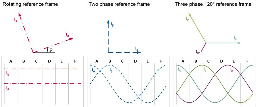
Sensorless Field Oriented Control with Embedded Power SoC
Z8F68474109

1 Introduction

1                  Introduction
The Field Oriented Control (FOC) method described in this document is aimed at the growing market for cost-
sensitive automotive drives, such as fans, pumps and geared motors. It is generally agreed that two main
vectors have been driving the adoption of FOC-driven three phase motors in the automotive market: system
cost and energy efficiency.
Sensors, indeed, require additional cost both for the sensing element and the required wiring harnesses and
connectors. This may generate problems in manufacturing and act as a source of faults, reducing reliability.
The other major vector is the significant improvement of energy efficiency of a motor. FOC methodology allows
for efficiency of up to 95%. This significantly reduces power consumption and improves motor dynamics, heat
dissipation and noise. For example many fans and pumps applications required silent operation, in order to
limit solid-borne sounds which eventually propagate in water or air pipes within the car cabin. Usually this
leads to control techniques resulting in sinusoidal currents in the motor coils.
The Infineon Embedded Power SoC (system-on-chip) devices allow the implementation of 3-phase motor
control ECUs optimized for both system size and cost. The SoC integrates the MCU and all necessary peripherals
on a monolithic IC, with only the power stage’s MOSFETs as additional external semiconductor devices. A major
feature is the integrated bridge driver with its innovative gate driver which simplifies development and system
optimization (e.g. improvement of EMC performance and adaptive capabilities to a wide range of different
power stages characteristics).

Application Note                                       5                                                 Rev 1.0
                                                                                                      2020-03-09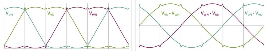
Sensorless Field Oriented Control with Embedded Power SoC
Z8F68474109

2 Theory of Sensorless Field Oriented Control

2                           Theory of Sensorless Field Oriented Control
This chapter is intended to give an overview about the theory of the sensorless FOC of permanent magnet
synchronous motors (PMSM). The control scheme which has been implemented with the TLE987x is based on
the theory described in this Chapter.
In these paragraphs the reader can find a summary about DC electrical motors and motor control, as well as a
description of FOC theory. Details about the TLE987x implementation of these algorithms are described in
Chapter Implementation of Sensorless FOC with the TLE9879 Embedded Power SoC.

2.1                         2-Phase (DC) Motor Basics
The 2-Phase motor, also known as DC motor, consists of a permanent magnet, which forms the stator structure,
and a coil wrapped around the rotor. A mechanical commutator, the so called “brushes” mechanism, is needed
in order to feed the current to the coils. This commutator will automatically switch the current orientation in
order to allow for the right torque generation in all rotor positions.

Figure 2                    DC Motor
The 2-Phase Motor is controlled by regulating the voltage amplitude at the brushes while the resulting current
is proportional to the torque of the motor. The speed of the motor depends on both the voltage and the torque.
The nominal speed (ω) and electric torque (Te) are defined in the following equations:

      ua − ia × Ra       ua − ia × Ra
        cE × ψf               kE
 ω=                  =

Equation 1

 Te = ct × ψf × ia = kT × ia

Equation 2
Where:
ua is the voltage applied to the rotor coil
ia is the current flowing through the rotor coil
Ra is the rotor’s coil resistance
cE, ct are the motor constants (usually identical)
ψf is the magnetic field flux linked to the coil’s defined area
KE is the electrical constant of the motor
KT is the mechanical constant of the motor
The time constants of speed and current control are different by orders of magnitude, hence a control cascade
structure for speed and current control can be utilized effectively.

Application Note                                        6                                                Rev 1.0
                                                                                                      2020-03-09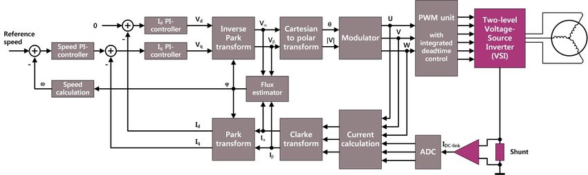
Sensorless Field Oriented Control with Embedded Power SoC
Z8F68474109

2 Theory of Sensorless Field Oriented Control

2.1.1                       2-Phase Motor Control: Open Loop Voltage Control
In an open loop voltage control, a reference voltage is input into the power stage, which will generate a given
voltage at the motor. The mechanical load influences the speed and the current of the DC motor.

Figure 3                    Open Loop Voltage Control
In steady state, the torque can be described by solving equation x and y which results in the following equation:

        ct × ψf            cE × ct × ψf2
 Te =      Ra
                  × ua −        Ra
                                           ×ω

Equation 3

2.1.2                       2-Phase Motor Control: Closed Loop Torque Control
The torque control loop requires the measurement of the motor current with a current sensor; e.g. a shunt
resistor. As seen in paragraph 2.1, in general the torque is proportional to the current .

 Te = kT × ia

Equation 4
Thus, the torque reference can be set by giving an input current reference. The actual current, measured by the
current sensor can be controlled with a PI controller in order to follow to the reference current. This will result in
the regulation of the reference voltage (Vref) for the power stage. Please see the following figure for details:

Figure 4                    Closed Loop Torque Control

Application Note                                          7                                                    Rev 1.0
                                                                                                            2020-03-09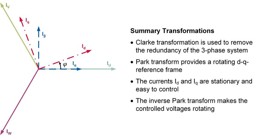
Sensorless Field Oriented Control with Embedded Power SoC
Z8F68474109

2 Theory of Sensorless Field Oriented Control

2.1.3               2-Phase Motor Control: Closed Loop Speed and Torque Control
As anticipated, a cascaded control structure can be used, because the speed change requirement is typically
much slower than the one for the current, hence for the torque. The speed control requires a speed sensor, e.g.
a tachometer, and the torque control requires a current sensor as seen in point 2.1.2. The output of the speed
control is the reference current for the current control. Usually a PI controller is used both for speed and current
control.

Figure 5            Cascaded Speed and Current Control

Application Note                                         8                                                    Rev 1.0
                                                                                                           2020-03-09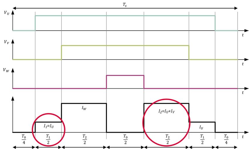
Sensorless Field Oriented Control with Embedded Power SoC
Z8F68474109

2 Theory of Sensorless Field Oriented Control

2.1.4                    List of Equations
The electrical equations of the DC motor are also valid for the 3-phase motor. In the following, a set of equations
is listed, which will be used later in this application note.

                   dia
 ua = Ra ia + La dt + ea

Equation 5               Voltage equation (for one phase)

 ea = cE ψf ω = kE ω

Equation 6               Induced voltage

 φ = ∫ωdt

Equation 7               Angle

 n = 60 2 π
         ω

Equation 8               Speed, in revolutions per minute (RPM)

Figure 6                 BLDC motor equivalent circuit

Application Note                                            9                                               Rev 1.0
                                                                                                         2020-03-09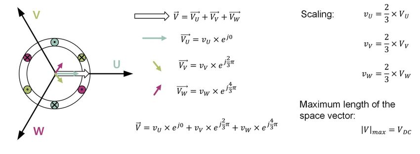
Sensorless Field Oriented Control with Embedded Power SoC
Z8F68474109

2 Theory of Sensorless Field Oriented Control

2.2                 3-Phase Motor Basics
Most 3-phase PMSM motors for low to medium power automotive application are also called BLDC motors. As
different terms are used in published literature, a short explanation and comparison amongst them will be
given.
The term BLDC stands for brushless DC motor. This term may lead to confusion at first glance, considering that
3-phase motors, including BLDC motors, require AC currents to be able to turn. However, this term is meant to
highlight the similarities between the two-phase (or DC) and three-phase BLDC electric motors. In fact, the
BLDC construction is similar in a key aspect: the torque equation of the BLDC is analogous to the one of the
brushed DC motor (see chapter 2-Phase Motor Control: Closed Loop Torque Control), as both are directly
proportional to current.
However, contrarily to the DC brushed motor, the BLDC is built with electromagnetic coils in the stator and
permanent magnets on the rotor – indeed it is often described as an “inside-out” DC motor. This construction
solves several of the disadvantages of the DC motor by substituting the mechanical commutation operated by
the brushed with electronic commutation served by a 3-phase bridge, also called inverter. Some of the typical
advantages of the BLDC motor are:
•    avoiding energy losses in the brushes
•    saving brush maintainance costs
• improved reliability by not having mechanical brushes at risk of failure
The term PMSM emphasizes the construction of the motor with coils in the stator and permanent magnets in
the rotor, as well as the fact that it rotates at a proportional speed to the coils alternating current’s frequency.
Since these properties are shared by the BLDC motor, some publications consider a BLDC a subtype of PMSM
motor.
In the industry, however, the terms BLDC & PMSM are often used in opposition to each other. The difference in
this usage is in the construction of the stator windings. The term BLDC motor is used for those which have
concentrated windings and surface mounted magnets while PMSM is used, more generally, when windings are
sinusoidally distributed or magnets aren’t surface mounted. This difference in the construction affects the flux
linkage between the magnet and the colis. This causes the back electro motive force (BEMF) voltage of the BLDC
to have a trapezoidal form while the BEMF of the PMSM is sinusoidal.

Application Note                                         10                                                  Rev 1.0
                                                                                                          2020-03-09
Sensorless Field Oriented Control with Embedded Power SoC
Z8F68474109
2 Theory of Sensorless Field Oriented Control
2.3 Space Vector Modulation
In this section, the modulation of a three leg voltage inverter is described. This type of inverter is made of six
MOSFETs or IGBTs which act as switches. The switches connected to the positive supply rail are called high-side
switches (HSS) and the switches connected to the negative rail of the power supply are called low-side switches
(LSS).
Figure 7 Three Leg Voltage Source Inverter
In the Figure 7 a block diagram of a three leg voltage source inverter can be seen. If we exclude states in which
the high and low switch of the same leg are turned on at the same time, as this would cause a short circuit,
there are eight states possible, as shown in Figure 9, each of them with different combinations of high and low
side switches active. In each of these states, the three phases would cause three different magnetic fields,
which can be visualized as vectors called magnetic dipoles. The combination of the effects of these fields can be
visualized as a combined field, resulting in the sum of the vectors as shown in Figure 8 in the form of complex
numbers.
Figure 8 Space Vectors in Comples Numbers
Thus, the states themselves can be associated to a resulting magnetic field expressed as a vector in the space
vector diagram of the coordinates U, V and W. There are two passive states leading to two null vectors, which do
not cause a magnetic field, and six active states represented by non-null vectors. These active vectors divide the
space vector diagram of a U-V-W system into six sectors, named A, B, C, D, E and F in Figure 9.
Application Note 11 Rev 1.0
2020-03-09Sensorless Field Oriented Control with Embedded Power SoC
Z8F68474109
2 Theory of Sensorless Field Oriented Control
Figure 9 Space Vector Diagram of a U-V-W System
Despite the fact that the stator coils are fixed in their position, the magnetic dipole rotates dependent on the
currents present in each phase. Considering any combination of voltages on the phases, their resulting
magnetic stator field (flux) may be expressed by a reference vector Vref. This one is defined by the following
equation:
V ref = V ref × ejφ
Equation 9
It is rotating in space with the speed (ω):
ω = 2π × f
Equation 10
This reference vector, if it is active, may be found in between any pair of the adjacent six active states, each of
which is called a sector. Any position of the reference vector in a sector may be approximated by a linear
combination of the two active vectors which define the sector (e.g. V1 and V2) and one zero vector (V0). The
attenuation factor needed for the two active vectors depends on the relative angle γrel, which is the absolute
angle φ minus the angle of the first active vector in the sector (according to a clockwise rotation convention).
This attenuation may be implemented physically by electrically changing the phase status significantly faster
than Vref changes. This means within a time Ts that we will call switching period, each one of the three active
vectors must be applied for a certain duration so that the average vector voltage represents Vref (see Figure 10).
This is the basis principle of pulse width modulation (PWM).
Application Note 12 Rev 1.0
2020-03-09Sensorless Field Oriented Control with Embedded Power SoC
Z8F68474109
2 Theory of Sensorless Field Oriented Control
Figure 10 Reference Vector Approximation
Taking into account the scaling of the reference vector and expressing the vector voltages as complex numbers,
the following equations are valid for the PWM on-time (time during which the HSSs are on) of a space vector
modulation:
V ref
T 1 = Ts V − γrel
π
DC
sin 3
Equation 11
V ref
T 2 = Ts V sin γrel
DC
Equation 12
T 0 = Ts − T 1 − T 2
Equation 13
The design of the switching sequence depends on the application requirements. Usually the number of
switchings is optimized in order to reduce switching losses.
The aim of the control is hence to calculate the duty cycle for each bridge phase that makes the Vref rotate with
the wanted electrical rotation.
Application Note 13 Rev 1.0
2020-03-09Sensorless Field Oriented Control with Embedded Power SoC
Z8F68474109
2 Theory of Sensorless Field Oriented Control
Figure 11 PWM Pattern of a Seven Segment Switching Sequence
An example of seven segment switching sequence during one PWM period Ts is shown in Figure 11. The output
voltage of each motor phase voltage vs neutral through the complete electrical rotation is shown in Figure 12.
The resulting voltages VUV, VUW and VVW at the motor are sinusoidal.
Figure 12 Output Voltage of Space Vector Modulation
Application Note 14 Rev 1.0
2020-03-09Sensorless Field Oriented Control with Embedded Power SoC
Z8F68474109
2 Theory of Sensorless Field Oriented Control
2.4 Phase Current Measurement
For many motor control schemes, the phase currents are required as input values. A cost efficient method
requires only one shunt in the DC-link. Two phase currents can be reconstructed from the DC-link current (IDC-
link) during one PWM period (Ts). The third phase current can be calculated by IU + IV + IW = 0, but is redundant for
the control. The current can be sampled with an ADC as shown in Figure 13.
Figure 13 Simplified current sensing schematic
Application Note 15 Rev 1.0
2020-03-09Sensorless Field Oriented Control with Embedded Power SoC
Z8F68474109
2 Theory of Sensorless Field Oriented Control
Figure 14 Phase Current Measurement within one PWM cycle in the SVM sector A.
In order to realize this method, the ADC trigger points must be adjusted according to the PWM pattern. Two
different currents I1 and I2 can be measured at PWM time T1 and T2. Depending on the actual SVM sector, the
measured currents I1 and I2 will have a different meaning. The following Table 2 shows these combinations and
the calculation for phase current IA and IB.
Table 2 Calculation for phase current IA and IB
Sector A,0 B,1 C,2 D,3 E,4 F,5
I1 IU IV IV IWW IVW IU
I2 IU+IV IU+IV IV+IW IV+IW IU+IW IU+IW
IA = IU I1 I2-I1 -I2 -I2 I2-I1 I1
IB = IV I2-I1 I1 I1 I2-I1 -I2 -I2
Application Note 16 Rev 1.0
2020-03-09Sensorless Field Oriented Control with Embedded Power SoC
Z8F68474109
2 Theory of Sensorless Field Oriented Control
2.4.1 Limitations of Phase Current Reconstruction
When T1 or T2 equals 0, only one phase current can be reconstructed. To avoid this situation, the PWM-times T1
and T2 have to be limited to a minimum value. This causes a ripple in the phase voltage and the phase current
as well. Figure 15 shows the output voltage and phase voltage of a T1-T2 -limited space vector modulation.
Figure 15 Space vector diagram with limitations caused by low duty cycles
Although the output signal is slightly distorted, the most cost efficient method of phase current measuring is
the reconstruction from the DClink current via a single shunt. A very fast ADC is required to optimize the system
performance. A direct trigger from the PWM unit to the ADC reduces CPU load significantly.
Figure 16 Distortion in Output and Motor Voltage
Application Note 17 Rev 1.0
2020-03-09Sensorless Field Oriented Control with Embedded Power SoC
Z8F68474109
2 Theory of Sensorless Field Oriented Control
2.5 FOC Calculations
FOC is a method which generates a three phase sinusoidal modulation, which can easily be controlled in
frequency and amplitude in order to minimize the currents and therefore maximize the efficiency. The essential
idea is the transformation of three phase sampled current signals into two rotor-fixed signals and vice versa. In
the rotor-fixed reference frame, the currents can be treated as stationary values and are easy to control. Using
the inverse vector rotation the controller generated reference voltages can be returned to a rotating vector in
the stator reference frame.
2.5.1 Stationary and Rotating Reference Frames
Figure 17 Stationary and Rotating Reference Frames
The transformation from the three phase system to the two phase system is called the Clarke transform,
whereas the one from stationary to rotating two-phase system is called the Park transform. These
transformations are expressed by the following equations:
Clarke Transform
iα = iU
Equation 14
iβ = i
3 U
+ 2iV
1
Equation 15
iU + iV + iW = 0
Equation 16
Park Transform
id = iα cos φ + iβ sin φ
Equation 17
Application Note 18 Rev 1.0
2020-03-09Sensorless Field Oriented Control with Embedded Power SoC
Z8F68474109
2 Theory of Sensorless Field Oriented Control
iq = −iα sin φ + iβ cos φ
Equation 18
Inverse Park Transform
iα = id cos φ − iq sin φ
Equation 19
iβ = −id sin φ + iq cos φ
Equation 20
Figure 18 Summary of Transformations
Application Note 19 Rev 1.0
2020-03-09Sensorless Field Oriented Control with Embedded Power SoC
Z8F68474109
2 Theory of Sensorless Field Oriented Control
2.5.2 Sensorless FOC
Sensorless operation offers the great advantage of saving the costs for an encoder or other position sensor. In
order to achieve this, the motor’s rotor flux is utilized to calculate the rotation angle and thus estimate rotor
position. The rotor flux itself is calculated in the flux estimator, which extracts the back EMF from the applied
phase voltage by subtracting all voltage drops not associated with the back EMF. The rotor flux is then found by
integration of the estimated back-EMF. Sensorless algorithms are less reliable when the applied phase voltage
or measured current is inexact, such as for low speed operation.
Figure 19 Block Diagram of Sensorless Field Oriented Control
Figure 19 shows the block diagram of the sensorless FOC algorithm. In this example, the flux estimator’s input
signals are taken from the orthogonal two phase stator system with the index α and β. The output signal
represents the rotor angle.
The motor signals in the two phase stator system (α-β-system) are equivalent to the three phase system. As a
result, an ideal two phase motor can be assumed in the α-β-system. Then there are only two equations to
calculate. The Figure 20 shows the voltage equations of the motor in the α-β-system.
Figure 20 Voltage Equations of Ideal 2-phase Motor
Application Note 20 Rev 1.0
2020-03-09Sensorless Field Oriented Control with Embedded Power SoC
Z8F68474109
2 Theory of Sensorless Field Oriented Control
The flux of the stator (Ψsα and Ψsβ) contain the mutual inductance L × is and the flux of the rotor Ψp generated by
permanent magnet.
The stator voltage equations (vsα and vsβ) contains the resistance of the coil R × is and the derivative of the flux
of the stator (Faraday’s Law).
Integrating the voltage equations, we calculate the stator flux as follows:
Ψsα = ∫vsα − R isα dt
Equation 21
Ψsβ = ∫vsβ − R isβ dt
Equation 22
The flux of the rotor and hereby the orientation (angle φ) of the permanent magnet of the rotor is calculated by
insertion:
Ψpα = Ψsα − L isα = ∫vsα − R isα dt − L isα
Equation 23
Ψpβ = Ψsβ − L isβ = ∫vsβ − R isβ dt − L isβ
Equation 24
Ψpβ
Ψpα
φ = atan
Equation 25
The position of the rotor can be calculated by knowing the resistance R and inductance L of the motor. The
stator voltage vs is derived from the algorithm, and the current is needs to be measured in real-time.
Application Note 21 Rev 1.0
2020-03-09Sensorless Field Oriented Control with Embedded Power SoC
Z8F68474109
3 Implementation of Sensorless FOC with the TLE9879 Embedded Power SoC
3 Implementation of Sensorless FOC with the TLE9879
Embedded Power SoC
This chapter describes the implementation of a sensorless Field Oriented Control using the Infineon TLE9879
SoC. The TLE9879 integrates an ARM Cortex M3 32-bit microcontroller, digital peripherals, NVM memory and
analog power peripherals in a 7x7mm 48-pin VQFN package. Together with an external power stage (MOSFET B6
bridge) the complete motor controller ECU can be realized in a very small footprint.
The 3 PWM units, several timers and very fast and powerful ADC make the TLE9879 a perfect fit for a variety of
cost optimized motor control applications.
Figure 21 Block diagram of TLE9879
3.1 System overview
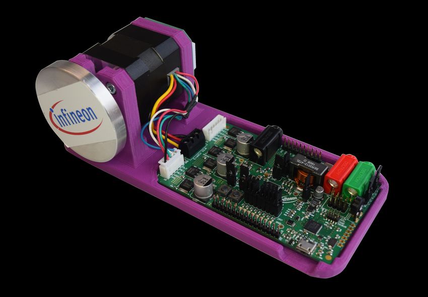
In typical applications for the TLE9879 SOC, the BLDC-Motor and the control ECU are mounted close to to each
other (Figure 21). The control ECU typically contains the TLE9879, next to six MOSFETs for the 3-phase bridge,
one MOSFET for reverse battery protection, and several passive components for protection, diagnosis and
filtering.
3.2 Hardware components of TLE9879
This chapter will explain the usage of the key hardware modules of TLE9879 for Sensorless FOC applications.
Application Note 22 Rev 1.0
2020-03-09Sensorless Field Oriented Control with Embedded Power SoC
Z8F68474109
3 Implementation of Sensorless FOC with the TLE9879 Embedded Power SoC
3.2.1 ADC
The ADC module is used to convert the current measurement from the shunt resistance at the DC-Link to a
digital value that can be used in the software. The measurement is performed twice during each PWM cycle, at
points where different phases are active, relying on the software’s knowledge of the implemented phase
modulation pattern. These two measurements allow for the calculation of two phases, whereas the third is
calculated by the equation iU+iV+iW=0. A critical aspect for the measurement is to complete it before the PWM
phase changes shifting to the next sector. This is achieved by starting the ADC measurement right after the
voltage ringing caused by the last PWM switching across the shunt resistor has subsided and with enough time
left to finish the measurement before the time of the measurement vector is over. Usually a good starting point
is right in the middle of the measurement vector.
Figure 22 ADC Measurement
3.2.2 GPT12E
In the example, the GTP1 timer is set up so that each step is 100ns, counting up to 1.8311ms. This is the timing
used by the speed pi controller in FOC.
Application Note 23 Rev 1.0
2020-03-09Sensorless Field Oriented Control with Embedded Power SoC
Z8F68474109
3 Implementation of Sensorless FOC with the TLE9879 Embedded Power SoC
3.2.3 CCU6
The CCU6 timer unit has beed designed to be able to generate the PWM signal by using both timers T12 and T13.
T12 is used to generate the signals for the Space Vector Modulation (SVM), which is why it has three different
compare values set on each single period. The timer’s period is setup according to the PWM frequency, whereas
the three compare values define the ON-time for the three phases. T13 is used in combination with T12 timing
to generate the trigger events for the ADC. T13 runs in single shot mode and starts automatically on one defined
compare match of one of the 3 compare channels. The generated trigger starts the conversion of the ADC1
channel which generates an interrupt after the channel is converted.
Additionally, the CCU6 can automatically add a deadtime. Depending on the MOSFET type used in the MOSFET
half-bridges, the switch-on and switch-off times will change. In the worst case, the switch-on time is smaller
than the time for switch-off and a short circuit in the inverter leg might occur. In order to guarantee safety of the
motor bridge, the capture / compare unit contains a programmable Dead-Time Generation Block which can
automatically add a delay between the switchoff on one MOSFET and the switch on of its compliment.
Please observe Figure 23 below.
Figure 23 PWM gate signals with dead-times (center-aligned mode)
Application Note 24 Rev 1.0
2020-03-09Sensorless Field Oriented Control with Embedded Power SoC
Z8F68474109
3 Implementation of Sensorless FOC with the TLE9879 Embedded Power SoC
3.2.4 BDRV
The MOSFET Driver is intended to drive external normal level MOSFETs built in a Bridge configuration. In our
case, the driver will deliver the physical implementation of the CCU6 signals.
The MOSFET driver is designed to drive N-MOSFETs due to them being standard in the industry. For this, the
MOSFET driver needs to supply voltages over the supply voltage, which is typically 12V for the TLE9879. This is
achieved through a two stage Charge Pump. The use of the charge pump enables a duty cycle range from 0 -
100%.
The regulated output voltage is typically VS + 14V (VS is typically the DC link voltage), but can be set to VS + 9V if
necessary. The charge pump output VCP is monitored via an undervoltage comparator. If undervoltage is
detected, the pumping is stopped and the drivers will be switched off.
3.2.5 Shunt Resistor & CSA
As discussed in the chapter 2, the key measured variable in Sensorless FOC is the DC-link current across the
Shunt resistor. The TLE9879 example configuration uses a single shunt resistor, enabling a more cost-optimized
solution for most low- to-mid power loads in a car, which do not require high dynamic capabilities.
The resulting voltage is then measured by ADC1 via an internal current sense amplifier, an external anti-aliasing
low-pass filter (AAF) and a single shunt resistor as shown in Figure 24
Figure 24 Motor current measurement
For this measurement, the key elements to be considered are the following:
• In the TLE987X SOC the ADC input voltage should not be higher than 5V because of the reference voltage. It
means the voltage between shunt (VP – VN) should be less than 5V /GTOTAL. If not, the ADC input stage will
be saturated.
• The maximum allowed power dissipation of the shunt resistor should be higher than (IMOT,max)2 * RSH
The recommended value for the low-pass filter resistors RLP is application specific. Please see our
recommendations in the User Manual for a starting point. The filter should be designed to only filter out high
frequency noise transients, and should influence the measured currents as little as possible.
Application Note 25 Rev 1.0
2020-03-09Sensorless Field Oriented Control with Embedded Power SoC
Z8F68474109
4 Software Block Diagram
4 Software Block Diagram
Figure 25 is a schematic software block diagram of the sensorless FOC example algorithm provided by Infineon
for the TLE987X. It shows the major software components and focuses on their basic roles & connections. The
main elements, starting from the current measurement on the right side, are a single shunt-based phase
current measurement and reconstruction, a Clark transform that converts three-phase to two-phase, a Park
transform that converts a rotating magnetic field into a fixed field, a cartesian transformation for angle position,
a Flux Estimator to estimate the flux & rotor position, PLL to estimate and smoothen the angle position in the
next PWM cycle, three PI Controllers to control velocity and the two fixed currents, a polar transformation for
angle & amplitude to be input into to SVM, and the SVM to modulate the space vector in complex space into
physical outputs.
Figure 25 Software Block Diagram
A key feature of this software that can also be seen in this software block diagram is the existence of two
different modes in the software – open and closed loop mode. As discussed in the theory section, one key
weakness of sensorless software methods is that they rely on the BEMF, which is proportional to speed. Because
of this, the Infineon example software includes a switch: it starts in open loop using a ramp angle for its
modulation and after a configurable time, it switches to the closed loop and uses the estimated angle from the
PLL.
Application Note 26 Rev 1.0
2020-03-09Sensorless Field Oriented Control with Embedded Power SoC
Z8F68474109
4 Software Block Diagram
4.1 Phase current measurement and reconstruction
The phase current detection is based on a single shunt and obtains the currents with two samples in one PWM
period. The generation of the phases is based on comparison values at the Timer12 which operates in Center
Aligned Mode. During this process, two shunt current measurements take place as shown in the following
Figure 26.
Figure 26 PWM synchronize sampling point each Sector
As you can observe in Figure 26, these currents are sampled at two different times in the PWM cycle enabling
measurement of different currents. They take place approximately halfway between the modulation of two
phases which ensures the shunt current has stabilized. Figure 27 shows this timing is achieved by utilizing
Timer13 for this delay.
Application Note 27 Rev 1.0
2020-03-09Sensorless Field Oriented Control with Embedded Power SoC
Z8F68474109
4 Software Block Diagram
Figure 27 Current measurement and FOC calculation
Let’s analyse Figure 26 in more detail. For example, the first sampling in Sector0 measures the contribution of
currents. Therefore, the current of U phase becomes I 1 and the current of V phase becomes I 2 − I 1. The current
the only U phase current wether the second sampling measures the contribution of both U and V phase
of W phase is calculated by −I 2 according to IU + IV + IW = 0. This analysis can be performed for each invididual
sector, and the results can be found in Table 3 and Table 4.
Table 3 Reconstruction mapping table
IV = PhasCurr.A IV = PhasCurr.B IW (not named in SW)
Sector0 I1 I2-I1 -I2
Sector1 I2-I1 I1 -I2
Sector2 -I2 I1 I2-I1
Sector3 -I2 I2-I1 I1
Sector4 I2-I1 -I2 I1
Sector5 I1 -I2 I2-I1
Table 4 The I1 and I2-I1 applied offset
Variable Formula Symbol Remark
R0mioffs = AdcResult0 - Emo_Svm.CsaOffsetAdw; I1 Measurement within T1
OffsmiR1 = Emo_Svm.CsaOffsetAdw - AdcResult1; -I2 Calculated
R1miR0 = AdcResult1 - AdcResult0; I2-I1 Measurement within T2
The variable definitions used by Infineon may seem arbitrary, they have constant properties over the PWM
cycle, which explain their usage:
Application Note 28 Rev 1.0
2020-03-09Sensorless Field Oriented Control with Embedded Power SoC
Z8F68474109
4 Software Block Diagram
• "R0mioffs" is a stable positive current
• "OffsmiR1" is negative
• "R1miR0" is close to zero
as seen in Figure 28.
Figure 28 Phase current reconstruction
Once this mechanism is understood, the reconstruction process can be seen as the simple selection of the
correct variable during each sector. For example, in order to reconstruct the U phase current, the positive
current in sector 0, the neutral current in sector 1, the negative current in sector 2 and 3, the netural current in
sector 4, the positive current in sector 5 are necessary.
Application Note 29 Rev 1.0
2020-03-09Sensorless Field Oriented Control with Embedded Power SoC
Z8F68474109
4 Software Block Diagram
4.2 Clarke Transform
As seen in the theory, the Clarke Transform converts the phase current stationary three-phase coordinate
system into a two-phase stationary coordinate system (α, β), simplifying the control. It is essentially a projection
into a Cartesian two-axis reference system. The factor 2/3 (marked in red) is required to keep the amplitude of
the space vector in Cartesian coordinates at the same value as the amplitude of the original phase value.
α = fa . cos0° − fb . cos60° − fc . cos60°
α′ = fa − fb 2 − fc 2 = fa − fb + fc = fa − −fa
1 1 1 1
2 2
α = 2 fa* 3 = fa
3 2
β = fa . sin0° + fb . sin60° − fc . sin60°
β′ = fb − fc fb − fc
3 3 3
2 2
= 2
β= fb − fc * 3 = fb − fc
3 2 1
2 3
Finally equation:
α = fa
β= 2fb − fa
1
3
Equation 26 Clarke transform fomula
In the software, this responsability is handled by the Mat_Clarke function. Figure 29 visually shows the result of
simulating this function, which transforms a three-phase coordinate system into a two-phase coordinate
system.
Input: 3phase current Output: α, β
Figure 29 Clarke transform in PLECS
Application Note 30 Rev 1.0
2020-03-09Sensorless Field Oriented Control with Embedded Power SoC
Z8F68474109
4 Software Block Diagram
4.3 Park Transform
As stated in the theory, the Park Transform converts a two-variable fixed coordinate system to a two-variable
rotating coordinate system. This means it transforms time-variant (AC) into time-invariant (DC) variables,
simplifying control. The angle between the fixed and the rotating systems is the angle of the rotor θ.
d = α . cosθ + β . sinθ
q = − α . sinθ + β . cosθ
Equation 27 Park transform formula
In the software, this responsability is handled by the Mat_Park function. Figure 30 visually shows the result of
simulating this function, which transforms a fixed coordinate system to the rotating coordinate system.
Input: α, β Output: d, q
Figure 30 Park transform in PLECS
Application Note 31 Rev 1.0
2020-03-09Sensorless Field Oriented Control with Embedded Power SoC
Z8F68474109
4 Software Block Diagram
4.4 Polar to Cartesian Transform
The flux estimator in the Infineon example software requires variables in Cartesian coordinates. This is a
standard mathematical transformation and its explanation is beyond the scope of this document.
α = Amp*cosθ
β = Amp *sinθ
Equation 28 Cartesian transform formula
In the software, this responsability is handled by the Mat_PolarKartesisch function. Figure 31 visually shows the
result of simulating this function, which transforms polar to Cartesian coordinates.
Figure 31 Cartesian transform in PLECS
Application Note 32 Rev 1.0
2020-03-09Sensorless Field Oriented Control with Embedded Power SoC
Z8F68474109
4 Software Block Diagram
4.5 Flux Estimator
As explained in the theory, in order to estimate the position of the rotor, the BEMF of the motor is calculated by
the flux estimator. The flux estimator is based on the RL motor circuit equation seen in Equation 29.
Estimating the flux linkage for α axis:
disα dΨsα
Vsα = Rs . isα + L dt
+ dt
Ψsα = ∫ V sα − Rs . isα dt − Ls . isα
Flux . Real
Estimating the flux linkage for β axis:
disβ dΨsβ
Vsβ = Rs . isβ + L dt
+ dt
Ψsβ = ∫ V sβ − Rs . isβ dt − Ls . isβ
Flux . Imag
Stator coordinates: Real-Imaginary to Module-
Phase conversion equations:
EmoFoc . FluxAngle = tan−1
Flux . Imag
Flux . Real
FluxAmp = Flux . Real2 + Flux . Imag2
Equation 29 Flux Estimator formula
In the Infineon example software the current values are the estimated currents in the stator coordinate system
(αβ) and the motor parameters are configured by the user during programming.
In the software, this responsability is handled by the emo_lEstFlux function. Figure 32 visually shows the result
of simulating this function, which estimates the angle.
Input: v_α, v_β, i_α, i_β Output: Angle
Figure 32 Flux Estimator in J-Scope
Application Note 33 Rev 1.0
2020-03-09Sensorless Field Oriented Control with Embedded Power SoC
Z8F68474109
4 Software Block Diagram
4.6 Angle PLL Observer
The main purpose of the PLL is to stabilize the angle position during the next PWM cycle based on measured
angle position, last known angle position and estimated speed. As shown in Equation 30, the PLL is
implemented via a regulation loop, which filters the angle output.
The P-Controller of the PLL should be dimensioned as follows: fast enough to follow the maximum expected
system dynamics, but slow enough to filter out angle errors caused by high frequency disturbances. Getting an
optimal solution to this problem usually requires testing on the complete system.
FluxAnglepll = Speedpll + pllkp∫φ t dt
FluxAngle: estimated angle
∆ φ: error of angle
ω: estimated angular velocity
FluxAnglepll : output angle
Equation 30 Angle PLL Observer
In the software, this responsability is handled by the Emo_FluxAnglePll function. Figure 33 visually shows the
result of simulating this function, which produces a smoother angle estimation (in green).
Application Note 34 Rev 1.0
2020-03-09Sensorless Field Oriented Control with Embedded Power SoC
Z8F68474109
4 Software Block Diagram
Input: FluxAngle, Speedpll Output: FluxAnglepll
Figure 33 PLL controller in J-Scope
Application Note 35 Rev 1.0
2020-03-09Sensorless Field Oriented Control with Embedded Power SoC
Z8F68474109
4 Software Block Diagram
4.7 PI Controller
Infineon’s example software includes two PI Controllers, which regulate the torque and speed in the motor drive
system. PI controllers combine the proportional controller and the integral controller to eliminate the steady
state error of proportional controllers while obtaining their quick response characteristics.
Control input: U t = K pe t + K i∫e t dt
R s : target value
E s : error
U s : control input
Y s : control output
Gc s : controller
Gp s : system
Equation 31 PI controller formula
In the software, this responsability is handled by the Mat_ExePi function. Figure 34 compares the control input
and output values for a PI controller.
Figure 34 PI controller in time domain
Application Note 36 Rev 1.0
2020-03-09Sensorless Field Oriented Control with Embedded Power SoC
Z8F68474109
4 Software Block Diagram
4.8 Cartesian to Polar Transform
The SVM module in the Infineon example software requires variables in polar coordinates. This is a standard
mathematical transformation and its explanation is beyond the scope of this document.
Amp = α2 + β2
θ = tan−1
α
β
Equation 32 Polar transform formula
In the software, this responsability is handled by the Mat_CalcAngleAmp function. Figure 35 visually shows the
result of simulating this function, which transforms Cartesian to polar coordinates.
Input: α, β Output: amp, θ
Figure 35 Polar transform in PLECS
Application Note 37 Rev 1.0
2020-03-09Sensorless Field Oriented Control with Embedded Power SoC
Z8F68474109
4 Software Block Diagram
4.9 SVM (Space Vector Modulation)
Space Vector Voltage Modulation (Space Vector PWM) is aimed to represent the reference vector Vref ,
characterized by a certain amplitude and angle, as the superposition and scaling (simultaneous PWM
modulation) of two active vectors in the space vector diagram.
If the reference voltage vector is located in the
region (0 ≤ θ ≤ 60 °), the following formula is
established.
Re: V ref . cosθ . Ts = T1 . V 1 + T2 . V 2 . cos6
Im: V ref . sinθ . Ts = T2 . V 2 . sin60°
Re: V ref . cosθ . Ts = T1 . 3 V DC + T2 . 3 V DC
2 1
Im: V ref . sinθ . Ts = T2 . V
3 DC
1
From this equation, the allowed time of the valid
voltage vector and the zero voltage vectors is as
follows.
3 . V ref . Ts . sin 60° − θ
T1 = V DC
3 . V ref . sinθ . Ts
T2 = V DC
Finally equation:
T1 = Ts . ma . sin 60° − θ
T2 = Ts . ma . sinθ
T 0 = Ts − T 1 + T 2
3 . V ref
ma = V DC
Application Note 38 Rev 1.0
2020-03-09Sensorless Field Oriented Control with Embedded Power SoC
Z8F68474109
4 Software Block Diagram
It is possible to obtain the valid voltage vector and
the allowed time of the zero voltage vectors by
performing the same calculation for the remaining
sector Sector 2 to 6 regions.
Equation 33 SVM
In the software, this responsability is handled by the Emo_lExeSvm function. Figure 36 visually shows the result
of simulating this function, which transforms the valid voltage vector in polar coordinates into the modulation
scheme for producing the MOSFET outputs.
Figure 36 SVM in J Scope
Application Note 39 Rev 1.0
2020-03-09Sensorless Field Oriented Control with Embedded Power SoC
Z8F68474109
5 Example Software
5 Example Software
This section illustrates the practical aspects of using the Infineon example FOC software, such as which software
programs are necessary, and the general layout of the software as a collection of files.
5.1 Tool chain
5.1.1 Compiler suite
This example uses KEIL compiler uVision5 (ARM Compiler, V5.22).
5.1.2 Debugger
This example uses KEIL compiler uVision5 as a software debugger and both Segger J-L ink LITE CortexM- 5V and
XMC-LINK (KIT_XMC_LINK_SEGGER_V1) have been used as hardware debuggers.
5.1.3 SDK
5.1.4 ConfigWizard
This example uses Infineon’s Config Wizard to set the initial register value for each peripheral block. This
enables easy understanding of register functionality through a GUI as seen in Figure 37. The selected values are
then saved through the interface’s file menu into a file with the structure xxx_defines.h which will be used by
the SDK to setup the configuration registers of the compiled software.
Figure 37 Config Wizard GUI
Application Note 40 Rev 1.0
2020-03-09Sensorless Field Oriented Control with Embedded Power SoC
Z8F68474109
5 Example Software
5.2 Example code & project layers
The Infineon example code can be downloaded free-of-charge through the uVision5 menu as seen in Figure 38.
Please open the Pack Installer from the uVision5 Build Toolbar. In the left menu, from the Devices tab, select
“Infineon” and then in the “TLE987X Series” select the device you will be working with. In the right menu, from
the “Examples” tab, you can find and copy the “BLDC Sensorless FOC” code.
Figure 38 BLDC Sensorless FOC Example Location within the Keil uVision5 Pack Installer
The example software project consists of three main layers called “app”, “emo” and “Devices” as described in
Figure 39.
Application Note 41 Rev 1.0
2020-03-09Sensorless Field Oriented Control with Embedded Power SoC
Z8F68474109
5 Example Software
Figure 39 Software Project Layers
Application Note 42 Rev 1.0
2020-03-09Sensorless Field Oriented Control with Embedded Power SoC
Z8F68474109
5 Example Software
5.2.1 “App”
The “app” layer is left intentionally limited in functionality for users to implement further features in this layer
depending on their application’s requirements. Typical examples include communication and monitoring
software.
File Main functionality
main.c Core of the program, motor start/stop control
5.2.2 “Emo”
The files found in the “emo” layer are related to the motor control. These files may also be edited by the user in
order to modify motor behavior or monitor particular parts of the software.
File Main functionality
Emo.c FOC initialization example, FOC programming in
memory
Emo_cfg.c Configuration values from FOC Motor Parameter tab in
ConfigWizard
Emo_RAM.c FOC programming in RAM
Emo_speed_api.c Speed control function
Table.c Tables for mathemicatical operations such as:
Sin, Sin60, Cos, ArcTan
5.2.3 “Device”
Device related files are automatically installed both on the FOC example code and more generally, on all
software projects generated for the TLE987X and coded in KEIL uVision 5. These files contain initialization and
control functions provided in order to access the capabilities of each hardware module in the chip. If a user
wants to change or optimize device files, it is highly recommended recommend to copy the device files from
their original shared location into the project folder and update the files. To be able to edit the device files one
must modify their Properties and uncheck the “read only” check box.
File Main functionality
adc1.c / adc1.h Defines, initialization functions and control functions
for the ADC1
adc2.c / adc2.h Defines, initialization functions and control functions
for the ADC2
... Defines, initialization functions and control functions
for other hardware modules
Application Note 43 Rev 1.0
2020-03-09Sensorless Field Oriented Control with Embedded Power SoC
Z8F68474109
5 Example Software
5.3 FOC parameter configuration
The example software requires a minimal amount of FOC parameter configuration in order to run most motors.
The FOC parameter configuration can be performed via the Configwizard GUI, in the FOC Motor Parameter tab.
This secton provides a simple explanation of the parameters in that tab.
Shunt Resist.[Ohm]: 5mΩ in eval kit
If other board: RShunt≤ 120mV/INOM
Nominal Current [A]: Max. expected peak phase
current
PWM Frequency [Hz]: 10~25kHz
PWM Period calculated depending on frequency
Phase Resistance [Ohm] & Phase Inductance [H]: As
measured, converted from star (/2) or delta (*1.5)
Pole Pairs & Max. Speed [rpm.mech.]: Determined by
motor
Current Controller Amplification: Scales current
control loop speed between 0.01 (slow) and 1 (fast)
Timer constant for Flux Estimator: KB for flux
estimator
Kp: Affects regulator speed
Ki: Affects regulator error
Speed Filter Time [s]: Low pass filter for speed,
between 0.01 (slow) and 1 (fast)
Switch-on Speed [rpm.mech.]: Beginning open loop
speed
End Start-up Speed [rpm,mech.]: Speed at end of
open loop
Start-up Acceleration [rpm/s,mech.]: Acceleration
during open loop
I/F initial Start Current [A]: Current limit during open
loop – see Figure 40
Rotor alignment time [s]: Time to place the rotor in a
known position before running – see Figure 40
Closed loop settings:
Direction dependent like many applications
FOC current for lower speeds [A]
Switch-over Speed [rpm,mech.]
FOC current for higher speeds [A]
Current limits for low and high speeds during closed
loop operation, and limit between the two - Figure 51
The setting of these parameters strongly depends on the respective motor characteristic and application
requirements. Infineon is happy to help customers find the correct parameters for their application.
Application Note 44 Rev 1.0
2020-03-09Sensorless Field Oriented Control with Embedded Power SoC
Z8F68474109
5 Example Software
Figure 40 Startup Behaviour
In case a customer would like to tune the FOC Parameter control, the following has been proven by Infineon’s
experience to be a useful algorithm:
1. Set Shunt Resistor, Norminal Current and PWM Frequency
2. Find and set motor parameters from motor data sheet
3. Set Kp, Ki and speed time in speed controller
4. Set Acceration ramp control (depending on motor and load condition)
5. Set rotor alignment time (set long time first, then reduce progressively)
6. Set Min/Max current in closed loop control and switch over speed
7. Repeat Step 3) to Step 6) to find the best fitting parameters.
Application Note 45 Rev 1.0
2020-03-09Sensorless Field Oriented Control with Embedded Power SoC
Z8F68474109
5 Example Software
5.4 How to Start
5.4.1 Test conditions
5.4.1.1 Test environment
The test environment consists of a TLE9879 evaluation kit, a J-Link Ultra+, a power supply and example code +
example code “BLDC_SENSORLESS_FOC_EXAMPLE_TLE987X” for Sensorless BLDC application.
Figure 41 Test environment
Application Note 46 Rev 1.0
2020-03-09Sensorless Field Oriented Control with Embedded Power SoC
Z8F68474109
5 Example Software
5.4.1.2 ConfigWizard parameters
Figure 42 Test case configwizard parameters
5.4.1.3 Startup test
Figure 43 shows how the motor operates after pressing the motor operation button MON1 to reach the
targetted RPM of 4000 RPM. After switching from EMO_MOTOR_STATE_STOP to EMO_MOTOR_STATE_START, the
motor increases its speed and then switches to EMO_MOTOR_STATE_RUN.
Figure 43 Startup test in J-Scope
Application Note 47 Rev 1.0
2020-03-09You can also read