Comparison of Calibration Approaches in Laser-Induced Breakdown Spectroscopy for Proximal Soil Sensing in Precision Agriculture - MDPI
←
→
Page content transcription
If your browser does not render page correctly, please read the page content below
sensors
Article
Comparison of Calibration Approaches in
Laser-Induced Breakdown Spectroscopy for Proximal
Soil Sensing in Precision Agriculture
Daniel Riebe 1 , Alexander Erler 1 , Pia Brinkmann 1 , Toralf Beitz 1 ,
Hans-Gerd Löhmannsröben 1, * and Robin Gebbers 2
 1   Physical Chemistry, University of Potsdam, Karl-Liebknecht-Str. 24-25, 14476 Potsdam, Germany;
     riebe@uni-potsdam.de (D.R.); aerler@uni-potsdam.de (A.E.); pbrinkma@uni-potsdam.de (P.B.);
     beitz@uni-potsdam.de (T.B.)
 2   Leibniz Institute for Agricultural Engineering and Bioeconomy (ATB), Max-Eyth-Allee 100,
     14469 Potsdam, Germany; rgebbers@atb-potsdam.de
 *   Correspondence: loeh@chem.uni-potsdam.de

 Received: 28 October 2019; Accepted: 25 November 2019; Published: 28 November 2019

 Abstract: The lack of soil data, which are relevant, reliable, affordable, immediately available, and
 sufficiently detailed, is still a significant challenge in precision agriculture. A promising technology
 for the spatial assessment of the distribution of chemical elements within fields, without sample
 preparation is laser-induced breakdown spectroscopy (LIBS). Its advantages are contrasted by a
 strong matrix dependence of the LIBS signal which necessitates careful data evaluation. In this work,
 different calibration approaches for soil LIBS data are presented. The data were obtained from 139
 soil samples collected on two neighboring agricultural fields in a quaternary landscape of northeast
 Germany with very variable soils. Reference analysis was carried out by inductively coupled plasma
 optical emission spectroscopy after wet digestion. The major nutrients Ca and Mg and the minor
 nutrient Fe were investigated. Three calibration strategies were compared. The first method was
 based on univariate calibration by standard addition using just one soil sample and applying the
 derived calibration model to the LIBS data of both fields. The second univariate model derived the
 calibration from the reference analytics of all samples from one field. The prediction is validated by
 LIBS data of the second field. The third method is a multivariate calibration approach based on partial
 least squares regression (PLSR). The LIBS spectra of the first field are used for training. Validation
 was carried out by 20-fold cross-validation using the LIBS data of the first field and independently on
 the second field data. The second univariate method yielded better calibration and prediction results
 compared to the first method, since matrix effects were better accounted for. PLSR did not strongly
 improve the prediction in comparison to the second univariate method.

 Keywords: laser-induced breakdown spectroscopy; LIBS; proximal soil sensing; soil nutrients;
 elemental composition

1. Introduction
      Precision agriculture (PA) requires reliable, affordable, immediately available soil data with
sufficient spatial and temporal resolution [1]. Soil maps for PA are typically derived from soil sampling
with subsequent laboratory analysis or from mapping with automated mobile proximal soil sensors.
Soil sampling and laboratory analysis is time consuming and becomes prohibitively expensive if
conducted on a fine grid [2]. As an alternative, mobile proximal soil sensors can measure several
hundred points (different locations) per hectare [3–7]. However, most of the current soil sensors

Sensors 2019, 19, 5244; doi:10.3390/s19235244                                   www.mdpi.com/journal/sensors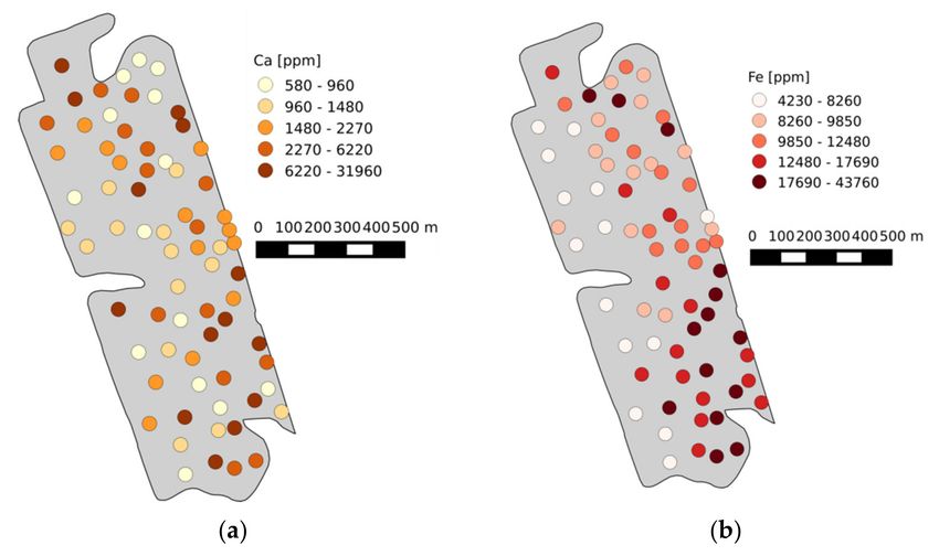
Sensors 2019, 19, 5244                                                                                 2 of 16

neither cover the whole range of soil fertility parameters nor do they directly measure them. The
automated mobile proximal soil sensing systems frequently used in practical PA as well as research
include geoelectrical, potentiometric pH, gamma-ray and spectral-optical sensors. Among these,
pH electrodes most directly access a soil fertility parameter, namely active acidity [8]. Gamma-ray
sensors detect radiation from K decay and from other isotopes. This can be correlated with K in
clay minerals and with plant available K+ [9,10]. Spectral-optical sensors include spectrometers
and multi-wavelength sensors in the visible and near-infrared region. Correlations with several soil
fertility parameters were observed, particularly with organic matter [11]. In research, visible and
near-infrared spectrometers were used to map several fertility parameters at the same time [12,13].
For practical applications, cheaper and more robust dual or multi-wavelength sensors for organic
matter and soil moisture were commercialized (e.g., by Veris Technologies and Precision Planting).
However, the relationships between optical soil properties and soil fertility parameters are variable
due to large overlaps of absorption bands. Thus, optical online sensors require careful calibration for
each field [11,14]. Geoelectric sensors traditionally formed the backbone of PA soil analysis efforts and
they are still widely used due to their robust nature making them both dependable and suitable for
field applications [15–17]. However, apparent soil electrical conductivity (ECa) is affected by many soil
parameters, including water content, texture, salinity, bulk density and temperature [18]. Therefore,
reference sampling in each field is required [19]. In a comparative study, Piiki et al. [20] recently
addressed the issue of obtaining as much direct information with as little calibration as possible. In that
study, X-ray fluorescence (XRF) spectroscopy produced the most reliable predictions of soil parameters
due to its direct detection of elemental compositions. XRF has gained interest in recent years due to
the availability of handheld sensors [21–23]. The drawbacks of XRF include the harmful X-rays, long
measurement times and the restriction to heavier elements.
      Laser-induced breakdown spectroscopy (LIBS) is a promising alternative to XRF for determining
element mass fractions in soils. In this method, an intense pulse of laser radiation is focused onto the soil,
where it ablates material from the surface and creates a microplasma. Subsequently, excited atoms and
ions in the plasma emit specific radiation which can be analyzed to elucidate the elemental composition
of the sample [24–28]. Ablation and plasma excitation are both highly complex phenomena. Since the
interaction of the laser radiation with the sample surface is influenced by its composition and structure,
a matrix-dependence of the signal response is observed. Matrix effects result from the light-to-sample
coupling, collisional interactions within the plasma, and plasma temperature, among others, all of
which influence the ratio of neutral and ionized species and self-absorption. These matrix effects and
spectral interferences were already investigated in different types of soil [29,30]. In LIBS soil analyses,
the whole spectrum of elements can be accessible. Depending on the calibration effort, elements can
be determined qualitatively or quantitatively. This allows the direct analysis of macro and micro
nutrients since no or only minimal sample preparation is necessary. In order to achieve the power
density required for plasma generation, the laser light pulse, of typically nanosecond duration, is
usually focused to a spot of about 10–500 µm diameter. As a consequence, the soil micro-heterogeneity
has to be considered in order to obtain representative results. This can be achieved by averaging
multiple spectra.
      Additional advantages of LIBS include the measurement speed, safety, as well as the portability of
the technique. These attributes make the method particularly interesting for on-site soil mapping. While
large-scale soil mapping applications of LIBS have not been reported yet and early LIBS investigations
of soils were focused on pollutants [31], the detection of nutrients in soils was already demonstrated in
some publications. Diaz et al. [32] were able to determine detection limits of P, Fe, Mg, Ca and Na by
univariate calibration in fertilizer/soil mixtures. Yongcheng et al. [33] could improve the prediction
of the Mg mass fraction by using a multivariate regression model that incorporates the lines of other
metals present in the soil. Nicolodelli et al. [34] investigated the feasibility of measuring C in soils
with a low resolution spectrometer. Rühlmann et al. [35] compare univariate and multivariate data
Sensors 2019, 19, 5244                                                                               3 of 16

evaluation approaches for the quantification of the nutrient Ca in reference soils. A review of recent
work on the application of LIBS for investigating agricultural materials can be found in [36].
      In this work, LIBS spectra of soils were measured in the laboratory as a fundamental study and
to provide a basis for the future application of LIBS directly on agricultural fields. The aim of the
study was the evaluation of different quantification approaches for LIBS data which consider the
matrix effect. Another goal was to explore how a calibration obtained for one field can be transferred
to another one. The accuracy of standard-free LIBS approaches [31,37] for the analysis of the very
complex matrix soil is still unsatisfactory. Therefore, the focus of this work was to compare different
univariate or multivariate calibration methods for the determination of nutrient mass fractions. The
target parameters of the investigation were the major nutrients Ca and Mg as well as the minor nutrient
Fe. One aim of this work was to examine whether the quantification of nutrients on the size scale of a
field can be carried out by univariate calibration or whether a multivariate method, namely partial least
squares regression (PLSR) has to be applied. Different calibration strategies, such as the generation of
calibration standards by standard addition to a single reference soil sample and the use of multiple
reference soil samples, were compared. The heterogeneity of the soil samples was characterized by
principal component analysis (PCA). The plasma was generated using UV radiation (355 nm), which
was recommended for soil investigations [30] in contrast to the widely applied NIR radiation (1064 nm).

2. Materials and Methods
      Soil samples and reference analysis. A total of 139 samples from two agricultural fields near the
village of Wilmersdorf in Northeast Germany (53◦ 060 N, 13◦ 540 E) were investigated. The regional
soilscape was formed by the last glaciation about 10,000 years ago and the following postglacial
processes. The parent material of the soil consists of calcareous glacial till covered by sandy deposits.
Soil texture varies between sand, loamy sand, and sandy loam in the topsoil. The main soil types
are alfisols. The samples were collected in 2011 to obtain reference data for proximal soil sensing as
published by Schirrmann, Gebbers and Kramer [14]. Reference analysis for elements was carried out
by inductively coupled plasma optical emission spectroscopy (ICP-OES) after aqua regia extraction by
a certified laboratory. As target parameters, Ca and Mg were selected as examples for major nutrients
and Fe as an example for minor nutrients.
      ECa mapping: ECa [mS/m] was mapped with a Veris 3100 system (Veris Technologies, Salina, KS,
USA) in 2011. Only data from the shallow measurement were used. Data were interpolated by block
kriging (a) on a regular grid for visualization and (b) on the sampling locations for correlation analysis.
      LIBS setup and measurement parameters. The plasma was created using a Nd:YAG laser
(Quanta-Ray, Spectra-Physics, Santa Clara, CA, USA, λ = 355 nm, E = 90 mJ). Emissions were collected
by a concave mirror, coupled into an optical fiber and guided to an echelle spectrometer (Aryelle
Butterfly, LTB, Berlin, Germany) equipped with an ICCD camera (iStar, AndorTechnology, Belfast, UK).
The spectrometer has two separate wavelength ranges (UV range: 190–330 nm, VIS range: 275–750 nm)
and a resolution of 20–30 pm. A total of 200 single shot spectra were recorded per sample in the UV as
well as in the VIS range. The sample holder was rotated and linearly translated during measurements
forming a spiral-like trace of ablation events. Optimization of LIBS spectra led to the following
measurement parameters: a detection delay of 2 µs, a measurement window of 10 µs as well as a
constant amplification factor of the iCCD camera.
      Sample treatment for LIBS. The soil samples were mixed with starch (19 wt% final mass fraction),
ground in an agate ball mill and subsequently pressed into pellets. One pellet was created for each
field sample point. For standard addition, the sample point of the first field with the lowest intensity
of the respective element peak was chosen for each investigated element. To that end, the soils were
mixed with the respective amounts of target elements added as salts (CaCO3 , MgCl2 and FeS, the
amount of starch was reduced in order to keep soil fraction constant) and also formed into pellets. The
salts were obtained from Sigma Aldrich (St. Louis, MO, USA).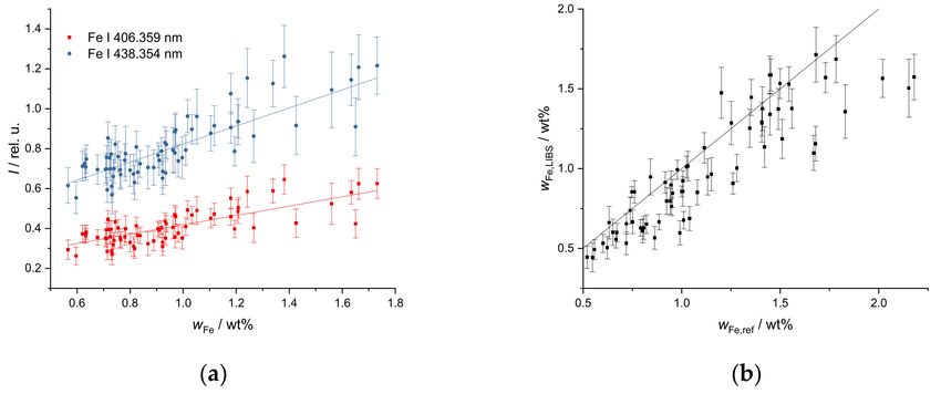
Sensors 2019, 19, 5244                                                                               4 of 16

       Data pretreatment. Pretreatment of the LIBS spectra consisted of outlier (e.g., spectra where
the laser did not fire) removal using the following procedure. The total intensity of each spectrum
for a given sample was calculated. The median of these values was derived and only the spectra in
the range 0.75 × median ≤ total intensity ≤ 1.25 × median were averaged to yield a single spectrum
for each soil sample. For PLSR calibration (third method, see below) spectra were mean centered.
Logarithms of the known element mass fractions were used as y variables when the data distribution
was strongly skewed. For univariate calibration, the peaks of investigated elements were integrated
for each averaged spectrum individually. For multivariate analysis, the entire spectra of either the UV
or the VIS region were used.
       Calibration. Standard addition univariate calibration. The first calibration method was based on
standard addition using just one soil sample and applying the derived univariate calibration model to
the LIBS data of both fields. Using the standard addition method potentially has several advantages.
First, the technique can be used to determine the mass fraction of one or several nutrients in one soil
sample by extrapolating the mass fraction of the base sample from the samples with added known
quantities of an element. Second, as applied in this work, reference analysis of the pure soil sample by
the traditional digestion method and in combination with samples where increasing amounts of the
nutrients were added can provide LIBS calibration curves. One additional benefit is that standard
addition yields response curves where the matrix effect of the local soil type is accounted for. The
nutrients are advantageously added as salts. However, care must be taken that the salts are not
hygroscopic. The third advantage is that the large range of nutrient mass fractions covered for the
determination of calibration curves facilitates assigning lines to elements and finding the best lines to
use for the quantification of each element. Potentially, different lines could be chosen for different mass
fraction ranges. The most intense lines might be useful at low element mass fractions, while at high
element mass fractions, these intense lines can be self-absorbed. Therefore, choosing weaker lines can
become beneficial.
       Reference univariate calibration. The second method derived a univariate calibration model from
the reference analytics of all samples from one field. The prediction is validated using the second field.
This approach accounts for the matrix effects even better, as the variation of the matrix across a field is
also reflected. Furthermore, the error in the laboratory-based reference analytics of one soil sample has
a large influence on the LIBS-based results. Therefore, a larger data pool with known reference values
and a broader variety of matrices should be regarded. In our case, the data of the first field is used for
the calibration and the data of the second field is used for the validation. The concept of this procedure
is that reference data gained in one year could be used to build a calibration for a specific field. In
subsequent years, it will not be necessary to take new samples and the calibration can therefore also be
applied to fields in the near surrounding and to fields with a similar soil type. Furthermore, a much
larger number of data points can be evaluated, as LIBS can be employed directly on the field, allowing
a closer spatial mapping of the fields.
       Reference multivariate calibration. The third approach was a multivariate calibration based on PLSR.
PLSR was done using the kernel algorithm and a maximum of 7 components. The LIBS spectra of the
first field were used for training. Validation was carried out by 20-fold cross-validation using the data
of the first field and independently by testing the model trained on the data of the first field with the
data of the second field.
       Software: Origin (OriginLab, Northampton, MA, USA) was used for PCA. Unscrambler X (Camo
Analytics, Oslo, Norway) was used to perform PLSR.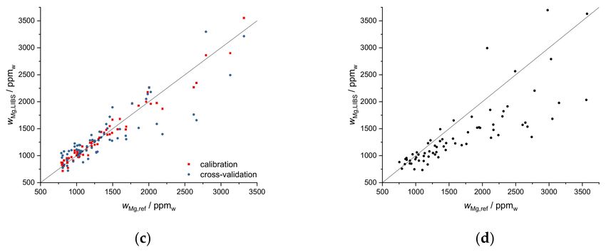
Sensors 2019, 19, 5244                                                                                     5 of 16

3. Results and Discussion

3.1. LIBS Spectra
     LIBS spectra of soils are rich in lines, mostly due to the presence of Fe and other transition metals
(Figure 1). Additionally, lines of most minor and major mineral nutrients are found, the lines of metal
nutrients are particularly intense.

      Figure 1. Typical soil laser-induced breakdown spectroscopy (LIBS) spectrum (composite of UV and VIS
      part of the LIBS spectrum), (a) full wavelength range, (b) detail view of wavelength range 400–450 nm.

     But the plethora of lines complicates their assignment to elements, as peak overlapping is
frequently observed. The line identification is not straightforward as the total elemental composition
of soils is generally not known. Otherwise, the limitation of the measurement campaign on one or
two fields is advantageous for peak assignment as the soil heterogeneity is not as great as on a larger
scale. Most peaks are generally found in spectra of all samples (different points on the field) but their
intensities still differ substantially on the scale of one field. This observation is due to variations of the
element mass fractions across the field, which is also the origin of the strong matrix effects encountered
and necessitates the determination of element distributions in precision agriculture.

3.2. Standard Addition Calibration
     Ca mass fractions vary greatly (from 500 ppmw to 5 wt%) in the investigated soils. A corresponding
calibration curve has to reflect a mass fraction range of nearly three orders of magnitude and is best
presented in a double-logarithmic diagram. The fitting function I = a wc , where I is line intensity, w the
mass fraction and a and c are the optimized constants, essentially equivalent to taking the logarithm
of the data prior to linear fitting, was used. The calibration curves for three different Ca lines (at
443.496 nm, 445.478 nm, 616.217 nm) are shown in Figure 2. These lines provided best results in
terms of repeatability (precision), linearity (R2 > 0.993) and usability over the entire range of relevant
mass fractions.
     The Fe mass fraction in the investigated soil (from 0.5 wt% to 6 wt%) is on a higher mass fraction
level but covers a narrower range than the Ca mass fraction. Thus, a linear calibration plot was selected
(Figure 3a). The LIBS spectrum contains a very high number of Fe lines. Due to the high mass fraction,
many of them show strong effects of self-absorption. This requires a careful selection of lines. The lines
at 406.359 nm and 438.354 nm (see Figure 3a) are best suited for calibration and yield R2 > 0.988 for
λ = 406.359 nm and R2 > 0.992 for λ = 438.354 nm. The repeatability is not as good as for Ca as the
error bars show, but quantification is still possible.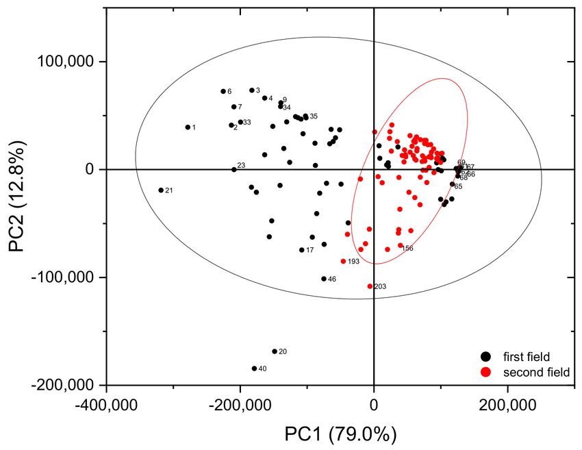
Sensors 2019, 19, 5244                                                                                       6 of 16

      Figure 2. Calibration curves of different Ca lines in soil, integrated line intensity over calculated Ca
      mass fraction: R2 (443.496 nm) = 0.994, R2 (445.478 nm) = 0.996, R2 (616.217 nm) = 0.993 (individual
      wavelengths are offset for visibility).

      Figure 3. Response curve of (a) FeS and (b) MgCl2 in soil, integrated line intensity over calculated
      (a) Fe and (b) Mg mass fractions, (a) R2 (406.359 nm) = 0.988, R2 (438.354 nm) = 0.992, (b) R2
      (277.983 nm) = 0.989.

    Mg appears in the soils at low to intermediate mass fractions (from 700 ppmw to 4000 ppmw )
and covers a narrow mass fraction range. Therefore, a linear calibration curve was selected as well.
Useful Mg lines are only found in the UV region. The repeatability is worse at higher mass fractions as
evidenced by higher error bars. The line at 277.983 nm shown in Figure 3b yields the best result in
terms of linearity over a range of mass fractions (R2 = 0.989).
    For all chosen elements, lines could be found in the available spectral range that are free from
overlap, less prone to self-absorption effects and provide good dynamic ranges. The detection limits
usually are in the range of 100 ppm which is adequate for the soils in question. Lower detection limits
would only be needed for micronutrients.

3.3. Application of Standard Addition Calibration to the First Field
     In order to obtain the mass fraction distribution of the nutrients on a field, the standard addition
calibration was applied to LIBS spectra of all samples (points on the field) for predicting the element
mass fractions. A comparison of the values thus obtained from the LIBS measurements and the
reference values obtained by ICP-OES yields insights into the performance of the calibration method.
This is shown for the nutrient Ca in Figure 4a, where the Ca mass fractions measured by LIBS are
the averages of the results for the three lines in the LIBS spectrum. The line in Figure 4a presents the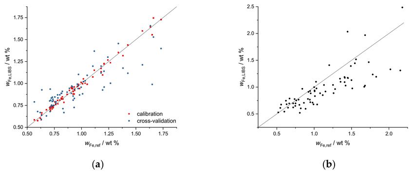
Sensors 2019, 19, 5244                                                                                     7 of 16

identity of values obtained by LIBS and ICP-OES. The Ca mass fractions obtained by LIBS scatter
around this line and show a very good agreement over the range of mass fractions investigated. Thus,
a univariate calibration, built using only one reference sample, can be used for predicting the Ca mass
fraction for the entire field. Absolute deviations for the different sample points on the field are shown
in Figure 4b with the highest errors in the range of 1%. The deviations seem accumulated around
certain points of the field as sample numbers indicate proximity. Because samples were taken along
predefined lines across the field, this could be an indication of different soil types and thus matrix
effects at those positions.

      Figure 4. (a) Mass fraction of Ca predicted by LIBS univariate calibration based on standard addition
      (wCa,LIBS ) compared to reference values obtained by ICP-OES upon aqua regia extraction (wCa,ref ) for
      the first field, R2 = 0.91, (b) deviation of predicted from reference value sorted by sample number.

     Results were not as promising for Fe (Figure 5a). Although a rough agreement is present in values
around 1 wt%, lower and especially higher Fe mass fractions are overestimated by as much as twice
the reference value. Reasons could be the relatively narrow range of mass fractions and especially the
high overall Fe mass fractions, leading to e.g., self-absorption. The results of the Mg prediction are
shown in Figure 5b. Agreement of the results is much better, although in the low mass fraction region,
a larger spread of the data points is observed. Overall, this kind of calibration is satisfactory for the
major nutrients Ca and Mg but the predictive power is limited for the minor nutrient Fe.

      Figure 5. Mass fractions of (a) Fe and (b) Mg predicted by LIBS univariate calibration based on
      standard addition compared to reference values obtained by ICP-OES upon aqua regia extraction for
      the first field.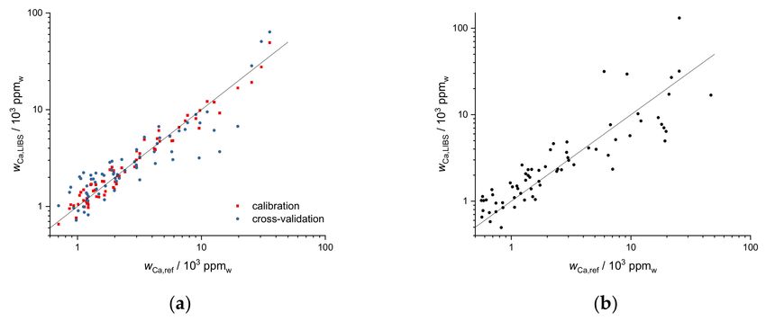
Sensors 2019, 19, 5244                                                                                      8 of 16

3.4. Application of Standard Addition Calibration to Second Field
      As a further validation, the same calibration curves were also applied to the second field data,
which does not contain the soil sample used for obtaining the standard addition calibration. Therefore,
the results of this second field are a measure of the predictive power for local agriculturally-used areas
in the surrounding of the calibration field. It is likely that the soil types on these fields will have a
similar characteristic.
      The prediction results of the three elements for both fields are similar (Figures 6 and 7). The
best agreements are again achieved for Ca and Mg, especially the correlation for Ca is excellent. The
prediction for Ca seems to be robust and can be also used for different fields of similar soil types. The
deviation of the Mg prediction (Figure 7) is a bit stronger than for the first field. While it could still be
usable in practice to get a rough estimation of the Mg mass fraction, a better method is desirable. The
agreement of the values of the second field in the Fe plot (Figure 6b) is actually better than for the first
field from which the soil for the calibration was taken, although the range of mass fractions is larger.
However, the deviation is still present, and the calibration can only be used as a rough estimation.

      Figure 6. Mass fraction of (a) Ca and (b) Fe predicted by LIBS univariate calibration based on standard
      addition compared to reference values obtained by ICP-OES upon aqua regia extraction for the second
      field, R2 (Ca) = 0.60.

      Figure 7. Mass fraction of Mg predicted by LIBS univariate calibration based on standard addition
      compared to reference values obtained by ICP-OES upon aqua regia extraction for the second field.

      Although the calibration method established from one sample works fine for the element Ca, even
on different fields, the applicability to other nutrients is limited. The most important reason for this
finding is the matrix effect, which is not sufficiently taken into account by this method. On a future
field campaign, the discussed peaks in the LIBS spectra can, however, be used to find points of extreme
element mass fractions, which are then crucial sampling points from which a better calibration can
be built.
Sensors 2019, 19, 5244                                                                                     9 of 16

3.5. Reference Univariate Calibration
     The results of the reference univariate calibration using all samples from the first field and its
application to the second field are shown below. The calibration data of the LIBS response for three
different wavelengths as a function of the Ca mass fraction obtained by the reference analysis are
shown in Figure 8a. For all wavelengths, a good regression (e.g., R2 (445.478 nm) = 0.94) between data
of the LIBS and reference analytical method is obtained, the coefficients of determination for the lines
at 443.496 nm and 445.478 nm are better than those for the line at 616.217 nm. The calibration curves
are applied to the LIBS data of the second field (Figure 8b), the Ca mass reported as measured by LIBS
are the averages of the results for the three lines. This procedure results in predicted values that are in
very good agreement with the reference data (R2 = 0.93).

      Figure 8. (a) Univariate calibration of Ca mass fraction calculated for data of the first field, R2
      (443.496 nm) = 0.93, R2 (445.478 nm) = 0.94, R2 (616.217 nm) = 0.86 (individual wavelengths are offset
      for visibility), (b) Calibration applied to the second field, R2 = 0.93.

     The same procedure was applied to Fe (Figure 9). The calibration plots (Figure 9a) took two
signals at the wavelengths at 406.359 nm and 438.354 nm into account but yielded a poorer prediction
than that found for Ca. However, the larger amount of data used for the calibration compared to the
standard addition method results in a better prediction for the second field (Figure 9b). Here, the
matrix effects are better accounted for. Although the result is acceptable, a univariate calibration might
not be ideal for Fe.

      Figure 9. (a) Univariate calibration of Fe mass fraction calculated for data of the first field, R2
      (406.359 nm) = 0.53, R2 (438.354 nm) = 0.61; (b) Calibration applied to the second field, R2 = 0.51,
      without two most obvious outliers (same samples as for Ca) R2 = 0.68.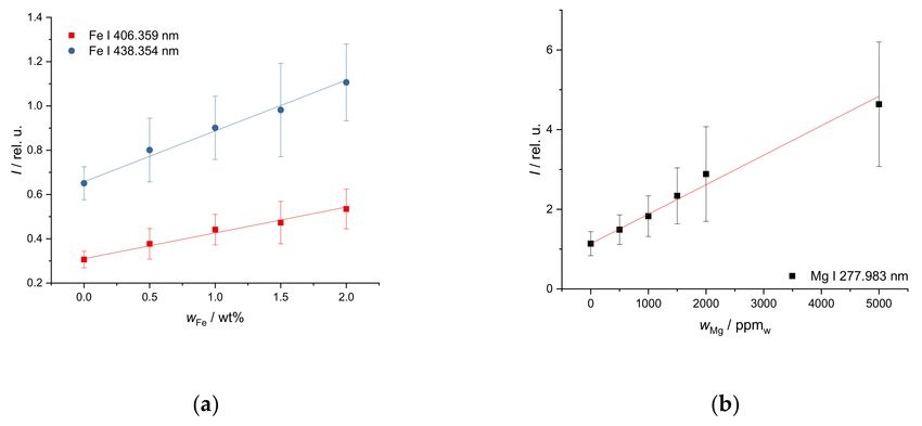
Sensors 2019, 19, 5244                                                                                        10 of 16

     While the calibration plot for Mg is characterized by a linear relationship but relatively large error
bars (Figure 10a), the validation plot (Figure 10b) obtained on the second field actually has a better
coefficient of determination than the calibration fit itself. Although this can be explained by a few high
error intervals of the intensities used for the calibration, it is still a promising result.

      Figure 10. (a) Univariate calibration of Mg mass fraction calculated for data of the first field, the line
      used is Mg I 277.983 nm, R2 = 0.71, (b) Calibration applied to the second field, R2 = 0.51, without two
      most obvious outliers (same samples as for Ca) R2 = 0.76.

     Overall, it can be concluded that using actual field samples for building the calibration improves
the performance for the univariate calibration. Such univariate methods can thus be used for predicting
values. In the future, online LIBS measurements on the field can be used to determine which samples
to use for laboratory analyses. If these samples represent a good range of the values of interest,
a strong calibration can be built, which can in turn be used to predict values for all points of the
online measurements.

3.6. Multivariate Analysis
     One possibility for characterizing the heterogeneity of soil compositions of the individual fields,
and of the first field in relation to the second field, is to apply PCA. For that purpose, the complete LIBS
spectra were introduced into PCA. In the score plot (Figure 11) the first two components, which explain
93% of the variance, are presented. Grouping the data points by fields implies that the heterogeneity of
the second field (red points) is lower than that of the first (black points). This also explains why the
univariate calibrations were largely successful and justifies using the first field as training data and the
second field as validation data in multivariate analyses.
Sensors 2019, 19, 5244 11 of 16
Figure 11. PCA of all LIBS spectra of the first (black points) and the second field (red points).
As a multivariate regression method, PLSR was performed on our data. Validation of the results
of the regression model was taken into account in two different ways. First, 20-fold cross-validation
was applied on the data of the first field. This is demonstrated for Ca data of the first field in Figure 12a.
Correlation plots of Ca mass fractions predicted by LIBS and by ICP-OES are shown. The red squares
are the result of the PLSR calibration, and the blue points represent 20-fold cross-validation. For PLSR,
the logarithms of Ca values were taken, and 5 components were used.
Figure 12. (a) Partial least squares regression (PLSR) of Ca data for the first field (UV range), red
squares represent calibration data (R2 = 0.96), blue points represent 20-fold cross-validation (R2 = 0.83),
(b) application of PLSR of Ca data to the second field (R2 = 0.58).
The PLSR cross-validation data (R2 = 0.83) demonstrate the potential of multivariate regression
for predicting mass fractions on the same field. A second, additional validation is obtained by applying
the calibration obtained of the first field to the second field, demonstrating how universal a calibration
could become. This is shown in Figure 12b for Ca and gives an impression of the prediction quality of
PLSR calibrations for additional fields with similar soil types (R2 = 0.58).
PLSR was also applied to the elements Fe and Mg (Figure 13). For both elements, the logarithms
of the mass fractions were used for PLSR. Seven components were used for PLSR of the Fe data, and 6
components were used for PLSR of the Mg data. The cross-validation plots of both elements scatter a
bit stronger than the Ca plot (R2 (Fe) = 0.70, R2 (Mg) = 0.79). The application of the calibration data
of the first to the second field results in a similar scattering of the predicted values. With increasingSensors 2019, 19, 5244 12 of 16
element mass fractions, the deviation of predicted values from reference values becomes systematically
larger. LIBS underestimates high Fe and Mg mass fractions.
Figure 13. (a) PLSR of Fe data for the first field (UV range), red points represent calibration data
(R2 = 0.986), blue diamonds represent 20-fold cross-validation (R2 = 0.70), (b) application of PLSR of Fe
data to the second field R2 = 0.37, (c) PLSR of Mg data for the first field (UV range), red points represent
calibration data (R2 = 0.96), blue diamonds represent 20-fold cross-validation R2 = 0.79, (d) application
of PLSR of Fe data to the second field R2 = 0.38.
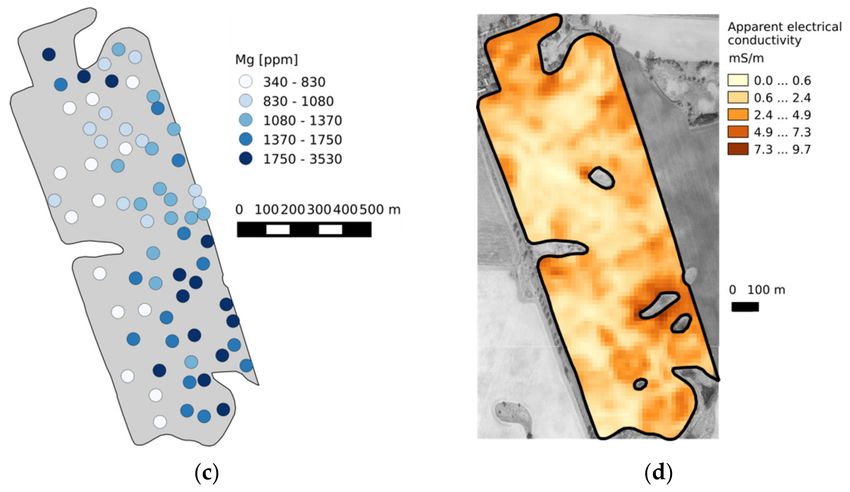
3.7. Field Maps
One main aim in precision farming is the mapping of nutrient distributions on agricultural fields.
In connection with fertilizer recommendations based on measured data as well as models, these maps
help the farmers identify nutrient-depleted areas. The change between nutrient-rich and depleted
areas can be seen on the three maps of Figure 14. Thus, the eastern areas are richer in all three elements
while the western areas are depleted.Sensors 2019, 19, 5244 13 of 16
Figure 14. Maps showing the element distribution of (a) Ca, (b) Fe, (c) Mg and (d) ECa on the first field
(north is up).
This spatial trend was further explained by the evaluation of the ECa map (Figure 14d), which
was recorded directly on the field. The ECa values were positively correlated with all elements as
determined by the reference method and by LIBS.
4. Summary and Conclusions
LIBS is a promising method for efficient soil data collection at high spatial resolution, as required
for precision agriculture. This is due to the capability of LIBS to rapidly measure mass fractions of
many elements simultaneously without or only very little sample preparation. These advantages are
contrasted by a strong matrix dependence of the LIBS signal which requires careful calibration and
data evaluation methods.
In this work, different approaches for the evaluation of LIBS data were investigated. The first
univariate method was based on standard addition to just one soil sample, the second was a univariate
method based on a larger number of samples characterized by reference analytics. This second
method accounted for matrix effects and thus yielded better predictions. The third method was a
multivariate method (PLSR) which yielded better calibration curves, but did not substantially improveSensors 2019, 19, 5244 14 of 16
the prediction compared to the reference univariate method. Alternative and maybe better suited
multivariate methods can potentially provide better results.
The work begun here should be continued by expanding the LIBS measurements to a larger
database, containing more and especially different soil types. It could also be interesting to obtain soil
samples from the same field in different years and verify if the same calibrations can be used. The
classification of soil samples based on different soil types and the application of tailored calibration
methods for these soil types can improve the accuracy and repeatability of measuring results in the
future. Additionally, the amount of sample preparation performed in this work has to be reduced in
order to transfer the method to the field.
Author Contributions: Conceptualization: D.R., T.B., H.-G.L. and R.G.; Data curation: D.R. and P.B.; Formal
analysis: D.R., Funding acquisition: D.R., T.B., H.-G.L. and R.G.; Investigation: D.R., A.E., P.B. and T.B.;
Methodology: D.R. and T.B.; Project administration: D.R., T.B., H.-G.L. and R.G.; Resources: H.-G.L. and R.G.;
Supervision: H.-G.L.; Visualization: D.R.; Writing—Original draft: D.R. and T.B. Writing—Review & editing:
H.-G.L. and R.G.
Funding: The authors gratefully acknowledge the financial support for this research received from the German
Ministry of Education and Research (BMBF) in the framework of the BonaRes project Integrated System for
Site-Specific Soil Fertility Management (I4S, grant no. 031A564H).
Acknowledgments: The authors would also like to thank Sascha Hons for support during the LIBS measurements.
We acknowledge the support of the Deutsche Forschungsgemeinschaft and Open Access Publishing Fund of
University of Potsdam
Conflicts of Interest: The authors declare no conflict of interest.
References
1. Stafford, J.V. Remote, non-contact and in-situ measurement of soil moisture content: A review. J. Agric. Eng.
Res. 1988, 41, 151–172. [CrossRef]
2. Viscarra Rossel, R.A.; McBratney, A.B. Soil chemical analytical accuracy and costs: Implications from
precision agriculture. Aust. J. Exp. Agric. 1998, 38, 765. [CrossRef]
3. Hummel, J.W.; Gaultney, L.D.; Sudduth, K.A. Soil property sensing for site-specific crop management.
Comput. Electron. Agric. 1996, 14, 121–136. [CrossRef]
4. Viscarra Rossel, R.A.; McBratney, A.B.; Minasny, B. (Eds.) Proximal Soil Sensing; Springer: Dordrecht, The
Netherlands, 2010.
5. Viscarra Rossel, R.A.; Adamchuk, V.I.; Sudduth, K.A.; McKenzie, N.J.; Lobsey, C. Proximal Soil Sensing: An
Effective Approach for Soil Measurements in Space and Time. In Advances in Agronomy; Academic Press:
Cambridge, MA, USA, 2011; pp. 243–291.
6. Viscarra Rossel, R.A.; Bouma, J. Soil sensing: A new paradigm for agriculture. Agric. Syst. 2016, 148, 71–74.
[CrossRef]
7. Gebbers, R. Proximal soil surveying and monitoring techniques. In Precision Agriculture for Sustainability;
Stafford, J., Ed.; Burleigh Dodds Science Publishing: Cambridge, UK, 2018; pp. 1–50.
8. Adamchuk, V.I.; Morgan, M.T.; Ess, D.R. An automated sampling system for measuring soil pH. Trans. ASAE
1999, 42, 885–891. [CrossRef]
9. Hyvönen, E.; Turunen, P.; Vanhanen, E.; Arkimaa, H.; Sutinen, R. Airborne Gamma-ray Surveys in Finland.
In Aerogeophysics in Finland 1972–2004: Methods, System Characteristics and Applications; Special Paper, 39;
Airo, M.-L., Ed.; Geological Survey of Finland: Espoo, Finland, 2005; pp. 119–134.
10. Heggemann, T.; Welp, G.; Amelung, W.; Angst, G.; Franz, S.O.; Koszinski, S.; Schmidt, K.; Pätzold, S. Proximal
gamma-ray spectrometry for site-independent in situ prediction of soil texture on ten heterogeneous fields in
Germany using support vector machines. Soil Tillage Res. 2017, 168, 99–109. [CrossRef]
11. Stenberg, B.; Viscarra Rossel, R.A.; Mouazen, A.M.; Wetterlind, J. Visible and Near Infrared Spectroscopy in
Soil Science. In Advances in Agronomy; Academic Press: Cambridge, MA, USA, 2010; pp. 163–215.
12. Shibusawa, S.; Sato, H.; Sasao, A.; Hirako, S.; Otomo, A. A Revised Soil Spectrophotometer. IFAC Proc. Vol.
2000, 33, 231–236. [CrossRef]
13. Schirrmann, M.; Gebbers, R.; Kramer, E.; Seidel, J. Soil pH mapping with an on-the-go sensor. Sensors 2011,
11, 573–598. [CrossRef]Sensors 2019, 19, 5244 15 of 16
14. Schirrmann, M.; Gebbers, R.; Kramer, E. Performance of Automated Near-Infrared Reflectance Spectrometry
for Continuous in Situ Mapping of Soil Fertility at Field Scale. Vadose Zo. J. 2013, 12, 1. [CrossRef]
15. Corwin, D.L. Past, present, and future trends of soil electrical conductivity measurement using geophysical
methods. In Handbook of Agricultural Geophysics; Allred, B.J., Daniels, J.J., Ehsani, M.R., Eds.; CRC Press: Boca
Raton, FL, USA, 2008; pp. 17–44.
16. Gebbers, R.; Lück, E.; Dabas, M.; Domsch, H. Comparison of instruments for geoelectrical soil mapping at
the field scale. Near Surf. Geophys. 2009, 7, 179–190. [CrossRef]
17. Heil, K.; Schmidhalter, U. The application of EM38: Determination of soil parameters, selection of soil
sampling points and use in agriculture and archaeology. Sensors 2017, 17, 2540. [CrossRef] [PubMed]
18. Corwin, D.L.; Lesch, S.M. Application of Soil Electrical Conductivity to Precision Agriculture. Agron. J. 2003,
95, 455. [CrossRef]
19. Adamchuk, V.I.; Viscarra Rossel, R.A.; Marx, D.B.; Samal, A.K. Using targeted sampling to process multivariate
soil sensing data. Geoderma 2011, 163, 63–73. [CrossRef]
20. Piikki, K.; Söderström, M.; Eriksson, J.; John, J.M.; Muthee, P.I.; Wetterlind, J.; Lund, E. Performance evaluation
of proximal sensors for soil assessment in smallholder farms in Embu County, Kenya. Sensors 2016, 16, 1950.
[CrossRef] [PubMed]
21. Zhu, Y.; Weindorf, D.C.; Zhang, W. Characterizing soils using a portable X-ray fluorescence spectrometer: 1.
Soil texture. Geoderma 2011, 167–168, 167–177. [CrossRef]
22. Gebbers, R.; Schirrmann, M. Potential of using portable x-ray fluorescence spectroscopy for rapid soil
analysis. In Precision Agriculture 0 15; Stafford, J.V., Ed.; Wageningen Academic Publishers: Wageningen, The
Netherlands, 2015; pp. 27–34.
23. Nawar, S.; Delbecque, N.; Declercq, Y.; De Smedt, P.; Finke, P.; Verdoodt, A.; Van Meirvenne, M.; Mouazen, A.M.
Can spectral analyses improve measurement of key soil fertility parameters with X-ray fluorescence
spectrometry? Geoderma 2019, 350, 29–39. [CrossRef]
24. Fortes, F.J.; Moros, J.; Lucena, P.; Cabalín, L.M.; Laserna, J.J. Laser-Induced Breakdown Spectroscopy. Anal.
Chem. 2013, 85, 640–669. [CrossRef]
25. Cremers, D.A.; Chinni, R.C. Laser-Induced Breakdown Spectroscopy—Capabilities and Limitations. Appl.
Spectrosc. Rev. 2009, 44, 457–506. [CrossRef]
26. Hahn, D.W.; Omenetto, N. Laser-Induced Breakdown Spectroscopy (LIBS), Part I: Review of Basic Diagnostics
and Plasma—Particle Interactions: Still-Challenging Issues within the Analytical Plasma Community. Appl.
Spectrosc. 2010, 64, 335A–336A. [CrossRef]
27. Hahn, D.W.; Omenetto, N. Laser-Induced Breakdown Spectroscopy (LIBS), Part II: Review of Instrumental
and Methodological Approaches to Material Analysis and Applications to Different Fields. Appl. Spectrosc.
2012, 66, 347–419. [CrossRef]
28. Zorov, N.B.; Popov, A.M.; Zaytsev, S.M.; Labutin, T.A. Qualitative and quantitative analysis of environmental
samples by laser-induced breakdown spectrometry. Russ. Chem. Rev. 2015, 84, 1021–1050. [CrossRef]
29. Popov, A.M.; Zaytsev, S.M.; Seliverstova, I.V.; Zakuskin, A.S.; Labutin, T.A. Matrix effects on laser-induced
plasma parameters for soils and ores. Spectrochim. Acta Part B At. Spectrosc. 2018, 148, 205–210. [CrossRef]
30. Zaytsev, S.M.; Krylov, I.N.; Popov, A.M.; Zorov, N.B.; Labutin, T.A. Accuracy enhancement of a multivariate
calibration for lead determination in soils by laser induced breakdown spectroscopy. Spectrochim. Acta Part B
At. Spectrosc. 2018, 140, 65–72. [CrossRef]
31. Ciucci, A.; Corsi, M.; Palleschi, V.; Rastelli, S.; Salvetti, A.; Tognoni, E. New Procedure for Quantitative
Elemental Analysis by Laser-Induced Plasma Spectroscopy. Appl. Spectrosc. 1999, 53, 960–964. [CrossRef]
32. Díaz, D.; Hahn, D.W.; Molina, A. Evaluation of Laser-Induced Breakdown Spectroscopy (LIBS) as a
Measurement Technique for Evaluation of Total Elemental Concentration in Soils. Appl. Spectrosc. 2012, 66,
99–106. [CrossRef]
33. Yongcheng, J.; Wen, S.; Baohua, Z.; Dong, L. Quantitative Analysis of Magnesium in Soil by Laser-Induced
Breakdown Spectroscopy Coupled with Nonlinear Multivariate Calibration. J. Appl. Spectrosc. 2017, 84,
731–737. [CrossRef]
34. Nicolodelli, G.; Marangoni, B.S.; Cabral, J.S.; Villas-Boas, P.R.; Senesi, G.S.; dos Santos, C.H.; Romano, R.A.;
Segnini, A.; Lucas, Y.; Montes, C.R.; et al. Quantification of total carbon in soil using laser-induced breakdown
spectroscopy: A method to correct interference lines. Appl. Opt. 2014, 53, 2170. [CrossRef]Sensors 2019, 19, 5244 16 of 16
35. Rühlmann, M.; Büchele, D.; Ostermann, M.; Bald, I.; Schmid, T. Challenges in the quantification of nutrients
in soils using laser-induced breakdown spectroscopy–A case study with calcium. Spectrochim. Acta Part B At.
Spectrosc. 2018, 146, 115–121. [CrossRef]
36. Nicolodelli, G.; Cabral, J.; Menegatti, C.R.; Marangoni, B.; Senesi, G.S. Recent advances and future trends in
LIBS applications to agricultural materials and their food derivatives: An overview of developments in the
last decade (2010–2019). Part I. Soils and fertilizers. TrAC Trends Anal. Chem. 2019, 115, 70–82. [CrossRef]
37. Herrera, K.K.; Tognoni, E.; Omenetto, N.; Smith, B.W.; Winefordner, J.D. Semi-quantitative analysis of metal
alloys, brass and soil samples by calibration-free laser-induced breakdown spectroscopy: Recent results and
considerations. J. Anal. At. Spectrom. 2009, 24, 413–425. [CrossRef]
© 2019 by the authors. Licensee MDPI, Basel, Switzerland. This article is an open access
article distributed under the terms and conditions of the Creative Commons Attribution
(CC BY) license (http://creativecommons.org/licenses/by/4.0/).You can also read