Route Planning with Real-Time Traffic Predictions - CEUR ...
←
→
Page content transcription
If your browser does not render page correctly, please read the page content below
Route Planning with Real-Time
                     Traffic Predictions

Thomas Liebig, Nico Piatkowski, Christian Bockermann, and Katharina Morik

                    TU Dortmund University, Dortmund, Germany,
                      {firstname.lastname}@tu-dortmund.de

        Abstract. Situation dependent route planning gathers increasing inter-
        est as cities become crowded and jammed. We present a system for indi-
        vidual trip planning that incorporates future traffic hazards in routing.
        Future traffic conditions are computed by a Spatio-Temporal Random
        Field based on a stream of sensor readings. In addition, our approach
        estimates traffic flow in areas with low sensor coverage using a Gaussian
        Process Regression. The conditioning of spatial regression on interme-
        diate predictions of a discrete probabilistic graphical model allows to
        incorporate historical data, streamed online data and a rich dependency
        structure at the same time. We demonstrate the system with a real-world
        use-case from Dublin city, Ireland.

        Resubmission of: [12] Predictive Trip Planning - Smart Routing in
        Smart Cities. In: Proceedings of the Workshops of the EDBT/ICDT 2014
        Joint Conference, vol. 1133, pp. 331–338. CEUR-WS.org (2014)

        Keywords: trip planning, real-time traffic model, traffic flow estimation

1     Introduction
The incentive for the creation of smart cities is the increase of living quality and
performance of the city. This is often accompanied with various mobile phone
apps or web services to bring new services to the people of a city – advertising
events, spreading city information or guiding people to their destinations by
providing smart trip planning based on the city’s spirit.
   With the unpleasant trend of growing congestion in modern urban areas,
smart route planing becomes an essential service in the smart city development.
Existing trip planning systems consider current traffic hazards and historical
speed profiles which are recorded by personal position traces and mobile phone
network data [19].
   The fast moving traffic situations in urban areas demand for a thorough
routing that incorporates as fresh information about the city’s infrastructure as
    Copyright c 2014 by the paper’s authors. Copying permitted only for private and
    academic purposes. In: T. Seidl, M. Hassani, C. Beecks (Eds.): Proceedings of the
    LWA 2014 Workshops: KDML, IR, FGWM, Aachen, Germany, 8-10 September 2014,
    published at http://ceur-ws.org

                                          83
possible. This current work, originally presented in [12], presents an approach to
situation dependent trip planning that incorporates real time information gained
from smart city sensors and combines this data with a model for estimating fu-
ture traffic situations for route calculation. The proposed system provides three
components: (1) an interactive web-based user interface that is based on the
popular OpenTripPlanner project [16]. The web interface allows for users to
specify start and target location and triggers the route planning and provides
a REST-ful service (REpresentation State Transfer, introduced in [18]) inter-
face to integrate such services into mobile applications. (2) A real-time backend
engine, based on the streams framework [3], which provides data stream pro-
cessing for various types of data. We provide input adapters for streams to read
and process SCATS data [1] emitted from automatic traffic loops (city sensors).
This allows us to maintain an up-to-date view of the city’s current traffic state.
(3) A sophisticated dynamic traffic model that is integrated into the backend
stream engine and which provides traffic flow estimation at unobserved locations
at future times.
The combination of these components is a trip planner that incorporates
the latest traffic state information as well as using a fine-grained future traffic
flow estimation for urban trip planning. We test our trip planner in a use case
scenario in the city of Dublin. The city is amongst the most jammed cities in
Europe The city holds about 966 SCATS sensors, each providing current traffic
flow and vehicle speed at the sensor location.
The paper is structured as follows. In the second section we describe the
general architecture of the presented system regarding the input and output
of the trip planner, the data analysis and the stream processing connecting
middleware. The third section deals with the application of our proposed trip
planner to a use case in Dublin, Ireland. In the fourth section we provide a
discussion of the work together with future directions. The fifth section presents
related work.
2 General Architecture
We give an overview of the system developed to address the veracity, velocity and
sparsity problems of urban traffic management. The system has been developed
as part of the INSIGHT project. This section describes the input and output of
the system, the individual components that perform the data analysis, and the
stream processing connecting middleware.
2.1 System Components
As already noted in the introduction, we built the system aiming real time
streaming capabilities. Based on the streams framework, the core engine is a data
flow graph that models the data stream processing of the incoming SCATS data.
This graph can easily be defined by means of the streams XML configuration
language and features the integration of custom components directly into the
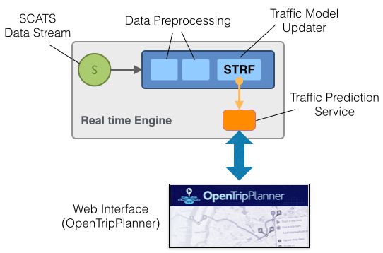
84data flow graph. As can be seen in Figure 1, this data flow graph contains
the SCATS data source as well as several nodes that represent preprocessing
operations. A crucial component within that stream processing is our Spatio-
Temporal Random Field (STRF) implementation1 , which is used in combination
with the sensor readings to provide a model for traffic flow prediction.
With the service layer API provided by streams, we export access to the traf-
fic prediction model to the OpenTripPlanner component. The OpenTripPlanner
provides the interface to let the user specify queries for route planning. Based on
a given query (v, w) with a starting location v and a destination w, it computes
the optimal route v → p0 . . . pk → w based on traffic costs. Here we plug in a
cost-model for the routing that is based on the traffic flow estimation and the
current city infrastructure status. This cost-model is queried by OpenTripPlan-
ner using the service layer API.
Fig. 1. A general overview of the components of the predictive trip planning system.
The real time engine continuously computes traffic condition forecasts and exports the
prediction service to the OpenTripPlanner. Best viewed in color.
2.2 Traffic Model
The key component of our system is the traffic model. It combines two machine
learning methods in a novel way, in order to achieve traffic flow predictions
for nearly arbitrary locations and points in time. This traffic model addresses
multiple facets of the trip planning problem:
– sparsity of stationary sensor readings among the city,
– velocity of real-time traffic readings and computation, and
– veracity of future traffic flow predictions.
Based on a stream of observed sensor measurements, a Spatio-Temporal Ran-
dom Field [17] estimates the future sensor values, whereas values for non-sensor
1
The C++ implementation of STRF and the JNI interface can be found at: http:
//sfb876.tu-dortmund.de/strf
85locations are estimated using Gaussian Processes [14]. To the best of the authors
knowledge, streamed STRF+GP prediction has not been considered until now
and is therefore a novel method for traffic modelling.
Spatio-Temporal Random Field for Flow Prediction In order to model
the temporal dynamics of the traffic flow as measured by the SCATS sensors
(Figure 3), a Spatio-Temporal Random Field is constructed. The intuition be-
hind STRF is based on sequential probabilistic graphical models, also known as
linear chains, which are popular in the natural language processing community.
There, consecutive words or corresponding word features are connected to a se-
quence of labels that reflects an underlying domain of interest like entities or part
of speech tags. If a sensor network, represented by a spatial graph G0 = (V0 , E0 ),
is considered that generates measurements over space and time, it is appealing to
identify the joint measurement of all sensors with a single word in a sentence and
connect those structures to form a temporal chain G1 − G2 − · · · − GT . Each part
Gt = (Vt , Et ) of the temporal chain replicates the given spatial graph G0 , which
represents the underlying physical placement of sensors, i.e., the spatial structure
of random variables that does not change over time. The parts are connected by
a set of spatio-temporal edges Et−1;t ⊂ Vt−1 × Vt for t = 2, . . . , T and E0;1 = ∅,
that represent dependencies between adjacent snapshot graphs Gt−1 and Gt ,
assuming a Markov property among snapshots, so that Et;t+h = ∅ whenever
h > 1 for any t. The resulting spatio-temporal graph G, consists of the snapshot
graphs Gt stacked in order for time frames t = 1, 2, . . . , T and the temporal edges
connecting them: G := (V, E) for V := ∪Tt=1 Vt and E := ∪Tt=1 {Et ∪ Et−1;t }.
Finally, G is used to induce a generative probabilistic graphical model that
allows us to predict (an approximation to) each sensors maximum-a-posterior
(MAP) state as well as the corresponding marginal probabilities. The full joint
probability mass function is given by
1 Y Y
pθ (X = x) = ψv (x) ψ(v,w) (x).
Ψ (θ)
v∈V (v,w)∈E
Here, X represents the random state of all sensors at all T points in time and x
is a particular assignment to X. It is assumed that each sensor emits a discrete
value from a finite set X . By construction, a single vertex v corresponds to a
single SCATS sensor s at a fixed point in time t. The potential function of an
STRF has a special form that obeys the smooth temporal dynamics inherent in
spatio-temporal data.
* t +
X 1
ψv (x) = ψs(t) (x) = exp Z s,i , φs(t) (x)
i=1
t−i+1
The STRF is therefore parametrized by the vectors Z s,i that store one weight
for each of the |X | possible values for each sensor s and point in time 1 ≤ i ≤ T .
The function φs(t) generates an indicator vector that contains exactly one 1
at the position of the state that is assigned to sensor s at time t in x and
86zero otherwise. For a given data set, the parameters Z are fitted by regularized
maximum-likelihood estimation.
As soon as the parameters are learned from the data, predictions can be
computed via MAP estimation,
x̂ = arg max pθ (xV \U | xU ), (1)
xV \U ∈X
where U ⊂ V is a set of spatio-temporal vertices with known values. The nodes
in U are termed observed nodes. Notice that U = ∅ is a perfectly valid choice
that yields the most probable state for each node, given no observed nodes. To
compute this quantity, the sum-product algorithm [10] is applied, often referred
to as loopy belief propagation (LBP). Although LBP computes only approximate
marginals and therefore MAP estimation by LBP may not be perfect [8], it
suffices our purpose.
Gaussian Process Model for Flow Imputation Based on the discrete es-
timates of the STRF, we model the junction based traffic flow values within a
Gaussian Process regression framework, similar to the approach in [14]. In the
traffic graph each junction corresponds to one vertex. To each vertex vi in the
graph, we introduce a latent variable fi which represents the true traffic flow at
vi . The observed traffic flow values are conditioned on the latent function values
with Gaussian noise i : yi = fi + i , i ∼ N (0, σ 2 ) .
We assume that the random vector of all latent function values follows a
Gaussian Process (GP), and in turn, any finite set of function values f =
fi : i = 1, . . . , M has a multivariate Gaussian distribution with mean and covari-
ances computed with mean and covariance functions of the GP. The multivari-
ate Gaussian prior distribution of the function values f is written as P (f |X) =
N (0, K) , where K is the so-called kernel and denotes the M × M covariance
matrix, zero mean is assumed without loss of generality.
For traffic flow values at unmeasured locations u, the predictive distribution
can be computed as follows. Based on the property of GP, the vector of ob-
served traffic flows (v at locations −u) and unobserved traffic flows (fu ) follows
a Gaussian distribution
K̂−u,−u + σ 2 I K̂−u,u
y
∼ N 0, , (2)
fu K̂u,−u K̂u,u
where K̂u,−u are the corresponding entries of K̂ between the unobserved vertices
u and observed ones −u. K̂−u,−u , K̂u,u , and K̂−u,u are defined equivalently. I
is an identity matrix of size | − u|.
Finally the conditional distribution of the unobserved traffic flows are still
Gaussian with the mean m and the covariance matrix Σ: m = K̂u,−u (K̂−u,−u +
σ 2 I )−1 y, Σ = K̂u,u − K̂u,−u (K̂−u,−u + σ 2 I )−1 K̂−u,u .
Since the latent variables f are linked together in a graph G, it is obvious
that the covariances are closely related to the network structure: the variables
87are highly correlated if they are adjacent in G, and vice versa. Therefore we can
employ graph kernels [23] to denote the covariance functions k(xi , xj ) among the
locations xi and xj , and thus the covariance matrix.
The work in [14, 13] describes methods to incorporate knowledge on preferred
routes in the kernel matrix. Lacking this information, we decide for the commonly
−1
used regularized Laplacian kernel function K = β(L+I/α2 ) , where α and β
are hyperparameters. L denotes the combinatorial Laplacian, which is computed
as L = D − A, where A denotes the P adjacency matrix of the graph G. D is a
diagonal matrix with entries di,i = j Ai,j .
2.3 OpenTripPlanner
OpenTripPlanner (OTP) is an open source initiative for route calculation. The
traffic network for route calculation is generated using data from OpenStreetMap
and (eventually) public transport schedules. Thus, OpenTripPlanner allows route
calculation for multiple modes of transportation including walking, bicycling,
transit or its combinations. However, vehicular routing is possible, but for data
quality reasons in OpenStreetMap concerning the turning restrictions [20] it is
not advisable. The default routing algorithm in OTP is the A∗ algorithm which
utilizes a cost-heuristic to prune the Dijkstra search.
OpenTripPlanner consists of two components an API and a web applica-
tion which interfaces the API using RESTful services. The API loads the traffic
network graph, and calculates the routes. The web application provides an inter-
active browser based user interface with a map view. A user of the trip planner
can form a trip request by selecting a start and a target location on the map.
2.4 The streams Framework
The need for real time capabilities in today’s data processing and the steady
decrease of latency from data acquisition to knowledge extraction or informa-
tion use from that data led to a growing demand for general purpose stream
processing environments. Several such frameworks have evolved – Storm, Kafka
or Yahoo!’s S4 engine are among the most popular open-source approaches to
streaming data. They all feature slightly different APIs and come with slightly
different philosophies. Focusing on a more middle-layer approach is the streams
framework proposed in [3], which aims at providing a light-weight high-level
abstraction for defining data flow networks in an easy-to-use XML configura-
tion. It comes with its own execution engine, but also features the transparent
execution of data flow graphs on existing engines such as Storm. We base our
decision for the streams framework on its recent applications that highlight its
high throughput capabilities [5] and the built-in data mining operators [2].
SCATS Data Processing with streams Within the streams framework, a
data source is represented as a sequences of data items, which in turn are sets of
key-value pairs, i.e. event attributes and their values. Processes within a streams
88data flow graph consume data items from streams and apply functions onto the
data. The data flow graph for manipulation, analysis and filtering of the streams
is formulated in an XML-based language that streams provides. A sample XML
configuration is given in Figure 2.
Fig. 2. XML representation of a streams container with a source for SCATS data and
a process that applies a normalization to each data item and then forwards it to a
traffic estimation processor.
The process setup of Figure 2 defines a single data source that provides a
stream of SCATS sensor data. A process is attached to this source and con-
tinuously reads items from that source. For each of the data item, it applies
a sequence of custom functions (so called processors) that reflect data trans-
formations or other actions on the items. In the example above, we include a
SCATS specific DataNormalization step as well as our custom TrafficEstimator
implementation directly into the data flow graph.
Service Level API The streams runtime provides a simple RMI-based service
invocation of data flow components that do provide remote services. The Traf-
ficEstimator defines such a remote interface and is automatically registered as a
service with identifier “predictor”. This allows service methods of that estimator
to be asynchronously called from outside the data flow graph, i.e. from within
our modified OpenTripPlanner component.
The service method that is defined by the TrafficEstimator is exactly the
cost-retrieval function that is required within the A∗ algorithm of the OpenTrip-
Planner:
getCost(x, y, t)
where x and y are the longitude and latitude of the location and t is the time at
which the traffic flow for (x, y) shall be predicted.
3 Empirical Evaluation
In this section we present the application of our proposed trip planner to a use
case in Dublin, Ireland. We used real data streams obtained from the SCATS
sensors of Dublin city. The stream was collected between January and April
89Fig. 3. Locations of SCATS sensors (marked by red dots) within Dublin, Ireland. Best
viewed in color.
2013 and comprises ≈ 9GB of data. The SCATS dataset includes 966 sensors,
see Figure 3 for their spatial distribution among the traffic network. SCATS
sensors transmit information on traffic flow every six minutes. The data set is
publicly available2 .
For the experiments in Dublin, the traffic network is generated based on the
OpenStreetMap3 data. In the preprocessing step the network is restricted to a
bounding window of the city size. Next, every street is split at any junction in
order to retrieve street segments. In result we obtain a graph that represents the
traffic network. The SCATS locations are mapped to their nearest neighbours
within this street network.
In the preprocessing step the sensor readings are aggregated within fixed
time intervals. We tested various intervals and decided for 30 minutes, as lower
aggregates are too noisy, caused by traffic lights and sensor fidelity.
The spatial graph G0 that is required for the STRF is constructed as k-
nearest-neighbor (kNN) graph of the SCATS sensor locations. In what follows,
a 7NN graph is used, since a smaller k induces graphs with large disconnected
components and a larger k leads to more complex models without improving
the performance of the method. The fact that no information about the actual
street network is used to build G0 might seem counterintuitive, but undirected
graphical models like STRF do not use or rely on any notion of flow. They
rather make use of conditional independence, i.e. the state of any node v can be
computed if the states of its neighboring nodes are known. Thus, the kNN graph
can capture long-distance dependencies that are not represented in the actual
street network connectivity. The maximum traffic flow value that is measured
by each SCATS sensor in each 30-minutes-window is discretized into one of
6 consecutive intervals. A separate STRF model for each day of the week is
2
Dublin SCATS data: http://www.dublinked.ie
3
OpenStreetMap: http://www.openstreetmap.org
90constructed and each day is further partitioned into 48 snapshot graphs, since we
can divide a day into 48 blocks of 30 minutes length. The model parameters are
estimated on SCATS data between January 1 and March 31 2013 and evaluated
using data from April 2013.
The evaluation data is streamed as observed nodes into the STRF which
computes a new conditioned MAP prediction (Equation 1) for all unobserved
vertices of the spatio-temporal graph G whenever time proceeds to the next
temporal snapshot. The discrete predictions are then de-discretized by taking the
mean of the bounds of the corresponding intervals and subsequently forwarded
to the Gaussian Process which uses these predictions to predict values at non-
sensor locations. Notice that although the discretization with subsequent de-
discretization seems inconvenient at a first glance, it allows the STRF to model
any non-linear temporal dynamics of the sensor measurements, i.e. the flow at a
fixed sensor might change instantly if the sensor is located close to a factory at
shift changeover.
Fig. 4. Results of route calculations for fixed start and target at different timestamps
(from left to right: 7:00, 8:00, 8:30). Best viewed in color.
Application of Gaussian Processes requires a joint multivariate Gaussian dis-
tribution among the considered random variables. In our case, these random
variables denote the traffic flow per junction. Literature on traffic flow theory
[11, 4] tested traffic flow distributions and supports a hypothesis for a joint log-
normal distribution. We test our dataset for this hypothesis. Thus, we apply the
Mardia [15] normality test to the preprocessed data set. The test checks multi-
variate skewness and kurtosis. We apply the implementation of the Mardia test
contained in the R package MVN [9]. The tests confirmed the hypothesis that
the recorded traffic flow (obtained from the SCATS system) is lognormal dis-
tributed. Thus, application of Gaussian Processes to log-transformed traffic flow
values is possible. The hyper-parameters for the GP are chosen in advance us-
ing a grid search. Best performance was achieved with α = 1/2 and β = 1/2. The
STRF provides complete knowledge on future sensor readings which is necessary
for our GP. As the STRF model performs well [17], we set the noise among the
sensor data in our GP to a small variance of 0.0001. For easy tractability, we set
up the GP to model about 5000 locations among the city of Dublin.
The OpenTripPlanner creates a query for the costs at a particular coordinate
in space-time. The query is transmitted from the route calculation to the traffic
model. There, the query is matched to the discrete space. The spatial coordinates
91are encoded in the WGS84 reference system. To avoid precision problems during
the matching between the components, the spatial coordinate is matched with a
nearest neighbour method using a KDTree data structure The nearest neighbor
matching offers also the possibility to query costs for arbitrary locations. The
timestamp of the query is discretized to one of the 48 bins we applied in the
STRF.
We apply our trip planner for a particular Monday in data set (8th April
2013) and compute routes from a fixed start to a fixed target at different time
stamps. Figure 4 shows that different routes are calculated depending on the
traffic situation. Congested street segments are avoided and different routes are
suggested.
4 Related Work
Previous sections already discussed related approaches. Here, we present briefly
recent work on dynamic cost estimation for trip planning in smart cities. Recent
work [24] predicts the travel time of routes. As their work evaluates a particular
predefined route based on recorded GPS traces, it has a related but different
scope. In contrast to [25], our approach combines the STRF with a GP for es-
timation of costs at unobserved locations. The approach in [6] addresses travel
time forecasts based on the delays in the public transportation system. Main
drawback of their method is that buses have extra lanes at most junctions and
their movement follows a regular pattern. The inclusion of traffic loop readings
was motivated in their section on future work. The dynamic traffic flow esti-
mation is a major problem in traffic theory. Common approach is the usage
of a k-Nearest Neighbour algorithm which calculates traffic flow estimates as
weighted average of the k nearest observations [7]. In contrast, our approach
models future traffic flow values based on their temporal patterns, correlations
and dependencies. Foremost, our model requires less memory as k-NN which has
to store all previously seen sensor values for continuous traffic flow estimation.
Another paper that compares two prediction models for traffic flow estimation is
presented in [21]. By combining a Gauss Markov Model with a Gaussian Process,
their work provides a faster model which is suitable for near time predictions
(as required for automatic signal control). The model estimates future values
by consecutive application of the model. In contrast, the hereby presented work
estimates all future time slices at once. In result, we built valuable trip planner
application on top of the traffic estimation model and highlighted its usability.
Improvement of the estimation method, and comparison of estimation accuracy
is subject for future work.
5 Discussion and Future Work
Within this paper we presented a novel approach for trip planning in highly con-
gested urban areas. Our approach computes intelligent routes that avoid traffic
hazards in advance. The proposed trip planner consists of a continuous traffic
92model based on real-time sensor readings and a web based user interface. We
combined the real-time traffic model and the trip calculation with a streaming
backbone. We applied the trip planner to a real-world use case in the city of
Dublin, Ireland.
Our traffic model combines latest advances in traffic flow estimation. On the
one hand, prediction of future sensor values is performed with a spatio-temporal
random field, which is trained in advance. Based on these estimates, the traffic
flow for unobserved locations is performed by a Gaussian Process Regression. We
successfully applied the Regularized Laplacian Kernel. In literature, also other
kernels have been successfully applied to the problem, [13, 22]. Exploration of
different kernel methods is subject for future research.
Besides the SCATS data also other data sources provide useful information
for dynamic cost estimation. The integration of bus travel times or user generated
(crowdsourcing and social network) data in our model is possible by dynamically
changing the traffic network (in case of road blockages) or introducing dynamic
weights (in case of a accident or flooding on a street segment). Future studies
need to explore these directions.
Acknowledgements This work is funded by the following projects: EU FP7
INSIGHT (318225); the Deutsche Forschungsgemeinschaft within the CRC SFB
876 Providing Information by Resource-Constrained Data Analysis, A1 and C1.
References
1. SCATS. Sydney Coordinated Adaptive Traffic System, Available:
http://www.scats.com.au/ [Last accessed: 27 June 2013] (2013)
2. Bockermann, C., Blom, H.: Processing Data Streams with the RapidMiner
Streams-Plugin. In: Proceedings of the 3rd RapidMiner Community Meeting and
Conference (2012)
3. Bockermann, C., Blom, H.: The streams framework. Tech. Rep. 5, TU Dort-
mund University (12 2012), http://jwall.org/streams/tr.pdf[Lastaccessed:
28November2013]
4. Davis, G.: estimation theory approach to monitoring and updating average daily
traffic. Tech. Rep. mn/rc 97-05, minnesota department of transportation, office of
research administration (january 1997)
5. Gal, A., Keren, S., Sondak, M., Weidlich, M., Blom, H., Bockermann, C.: Grand
challenge: The techniball system. In: Proceedings of the 7th ACM International
Conference on Distributed Event-based Systems. pp. 319–324. DEBS ’13, ACM,
New York, NY, USA (2013)
6. Gasparini, L., Bouillet, E., Calabrese, F., Verscheure, O., O’Brien, B., O’Donnell,
M.: System and analytics for continuously assessing transport systems from sparse
and noisy observations: Case study in dublin. In: Intelligent Transportation Sys-
tems (ITSC), 2011 14th International IEEE Conference on. pp. 1827–1832 (2011)
7. Gong, X., Wang, F.: Three Improvements on KNN-NPR for Traffic Flow Fore-
casting. In: Proceedings of the 5th International Conference on Intelligent Trans-
portation Systems. pp. 736–740. IEEE Press (2002), http://ieeexplore.ieee.
org/xpls/abs_all.jsp?arnumber=1041310&tag=1
938. Heinemann, U., Globerson, A.: What cannot be learned with bethe approxima-
tions. In: Proceedings of the 27th Conference on Uncertainty in Artificial Intelli-
gence. Barcelona, Spain (2011)
9. Kormaz, S.: MVN: Multivariate Normality Tests (2013), http://CRAN.R-project.
org/package=MVN, r package version 1.0
10. Kschischang, F.R., Frey, B.J., Loeliger, H.A.: Factor graphs and the sum-product
algorithm. IEEE Transactions on Information Theory 47(2), 498–519 (2001)
11. Lay, G.: Handbook of Road Technology, Fourth Edition. taylor & francis (2009)
12. Liebig, T., Piatkowski, N., Bockermann, C., Morik, K.: Predictive trip planning -
smart routing in smart cities. In: Proceedings of the Workshops of the EDBT/ICDT
2014 Joint Conference (EDBT/ICDT 2014), Athens, Greece, March 28, 2014. vol.
1133, pp. 331–338. CEUR-WS.org (2014)
13. Liebig, T., Xu, Z., May, M.: Incorporating mobility patterns in pedestrian quantity
estimation and sensor placement. In: Nin, J., Villatoro, D. (eds.) Citizen in Sensor
Networks, Lecture Notes in Computer Science, vol. 7685, pp. 67–80. Springer Berlin
Heidelberg (2013)
14. Liebig, T., Xu, Z., May, M., Wrobel, S.: Pedestrian quantity estimation with tra-
jectory patterns. In: Flach, P.A., Bie, T., Cristianini, N. (eds.) Machine Learning
and Knowledge Discovery in Databases, Lecture Notes in Computer Science, vol.
7524, pp. 629–643. Springer Berlin Heidelberg (2012)
15. Mardia, K.V.: Measures of multivariate skewness and kurtosis with applications.
Biometrika 57, 519–530 (1970)
16. McHugh, B.: The opentripplanner project. Tech. Rep. Metro RTO Grant Final
Report, TriMet (August 2011), http://portlandtransport.com/documents/OTP\
%20Final\%20Report\%20-\%20Metro\%202009-2011\%20RTO\%20Grant.pdf
17. Piatkowski, N., Lee, S., Morik, K.: Spatio-temporal random fields: compressible
representation and distributed estimation. Machine Learning 93(1), 115–139 (2013)
18. Richardson, L., Ruby, S.: RESTful Web Services. O’Reilly Series, O’Reilly Media,
Incorporated (2007), http://books.google.de/books?id=XUaErakHsoAC
19. Schäfer, R.P.: IQ Routes and HD Traffic: Technology Insights About Tomtom’s
Time-dynamic Navigation Concept. In: Proceedings of the the 7th Joint Meeting
of the European Software Engineering Conference and the ACM SIGSOFT Sym-
posium on The Foundations of Software Engineering. pp. 171–172. ESEC/FSE ’09,
ACM, New York, NY, USA (2009)
20. Scheider, S., Possin, J.: Affordance-based individuation of junctions in open street
map. Journal of Spatial Information Science 4(1), 31–56 (2012)
21. Schnitzler, F., Liebig, T., Mannor, S., Morik, K.: Combining a gauss-markov model
and gaussian process for traffic prediction in dublin city center. In: Proceedings of
the Workshop on Mining Urban Data at the International Conference on Extending
Database Technology. p. (to appear) (2014)
22. Selby, B., Kockelman, K.M.: Spatial prediction of traffic levels in unmeasured lo-
cations: applications of universal kriging and geographically weighted regression.
Journal of Transport Geography 29, 24–32 (May 2013)
23. Smola, A., Kondor, R.: Kernels and regularization on graphs. In: Proc. Conf. on
Learning Theory and Kernel Machines. pp. 144–158 (2003)
24. Wang, Y., Zheng, Y., Xue, Y.: Travel time estimation of a path using sparse tra-
jectories. In: KDD 2014. ACM (August 2014), http://research.microsoft.com/
apps/pubs/default.aspx?id=217493
25. Yang, B., Guo, C., Jensen, C.S.: Travel cost inference from sparse, spatio tem-
porally correlated time series using markov models. Proc. VLDB Endow. 6(9),
769–780 (July 2013), http://dx.doi.org/10.14778/2536360.2536375
94You can also read