WFC3/IR Filter-Dependent Sky Flats

Instrument Science Report WFC3 2021-01

 WFC3/IR Filter-Dependent Sky Flats
 J. Mack, H. Olszewksi, N. Pirzkal
 January 11, 2021

ABSTRACT
New ‘pixel-to-pixel’ P-flats have been derived from deep images of the IR sky background,
computed by stacking high signal-to-noise observations of sparse fields of view acquired over the
lifetime of WFC3. The new sky flats correct for wavelength-dependent residuals of ± 0.5% in the
central 800x800 pixel region of the detector and up to 2% near the detector edges. As of October
2020, these replace the prior 2011 set of P-flats, which were based on ground test data multiplied
by a smoothed ‘grey’ (filter-independent) correction derived from sky flats using the first 18
months of in-flight data. An accompanying set of ‘delta’ D-flats now correct for 148 catalogued
‘blobs’ in six IR filters as a function of the epoch of observation. These were computed by stacking
the same set of sky flat observations, but only after the appearance of each new blob.

I. Introduction

Flat field images for the WFC3/IR channel were produced in the laboratory prior to launch by
simulating the sky illumination with the CASTLE optical stimulus. These ‘pixel-to-pixel’ P-flat
reference files achieved signal-to-noise ~500, corresponding to errors of 0.2% per pixel from
Poisson counting statistics (Bushouse 2008). To test the accuracy of the ground flats using in-flight
data, dithered observations of the ACS calibration field in the outer region of 47 Tucanae were
acquired during Servicing Mission Observatory Verification program CAL-11453 in July 2009.
Aperture photometry revealed low-frequency sensitivity residuals of ± 1.5% across the detector in
all four filters, due to differences in the in-flight optical path (Hilbert et al. 2009).

To derive a ‘low-order’ L-flat correction to the P-flats, observations of the core of Omega-Cen
were acquired at several epochs between December 2009 and July 2011 in programs CAL-11928
and CAL-12340. This new target was selected because of its higher density and more uniform
distribution of sources across the field of view. Photometric residuals derived from these dithered
data showed peak-to-peak variations of ± 2.5% in a ‘wide cross shaped pattern’ for all filters,

 1

computed in grid of 16x16 boxes (64 pixels in width) across the detector (Pirzkal et al. 2011).
Unfortunately, the complex shape of the sensitivity residuals and the relatively low density of
bright sources meant that the star cluster data would not be useful to correct fine-scale spatial
structure with the required ~1% accuracy.

Observations of the moonlit Earth acquired in late 2010 (CAL-11917) confirmed that the extended
cross-shaped pattern was only introduced into FLT images calibrated using the ground flats. The
spectrum of the dark Earth is expected to have many bright emission lines, primarily due to OH
molecules in the mesosphere, and as such will be quite different than the spectrum of astronomical
sources or the zodiacal light. Thus ‘dark Earth’ calibration data were not used to derive a correction
to the ground flats. (They have been instead used to monitor the appearance of low sensitivity
artifacts known as ‘blobs,’ cf. McCullough et al. 2014).

Pirzkal et al. (2011) used long exposures of sparse astronomical fields to compute deep images of
the sky background in six IR filters. These ‘sky flats’ showed sensitivity residuals for all filters
which were consistent in both shape and in amplitude to within ~1%, excluding the detector edges.
The authors therefore computed a much higher signal-to-noise ‘grey’ correction by stacking
images in all filters. Their solution was heavily weighted toward F160W, because that filter
constituted nearly half of the observations. The ‘grey’ correction was then smoothed to reduce
noise and multiplied by each P-flat, providing a total correction of ~4% peak-to-peak. The updated
set of P-flat reference files are hereafter referred to collectively as the ‘P2011 flats’.

Bushouse (2008) attributed the flat field’s cross-like pattern to “the fact that the obscurations of
the optical stimulus, which supplied the external flat field illumination are not in a conjugate plane
to the cold mask in the WFC3 IR detector housing. The stimulus structures and WFC3 cold mask
structures, notably the spiders, thus move relative to each other as a function of field position,
causing variations in the illumination pattern.” Because the pattern was an artifact of the optical
stimulus, the authors predicted that it would not be present in on-orbit IR images and would
therefore need to be corrected in the flats. They also noted that particulates on the Channel Select
Mechanism (CSM) would be shifted inflight once the on-orbit optical alignment was performed,
and that the features referred to as ‘blobs’ would also need to be corrected.

To test the accuracy of the P2011 flats, the “WFC3/IR Spatial Sensitivity” program (CAL-12708)
acquired images of the standard star WD-1057+719 in F098M, F125W, and F160W, dithered
across the detector in a 21-point grid, to measure the photometric repeatability. For each grid
position, two images offset by ∼40 pixels were acquired to mitigate persistence. The typical rms
in the measured photometry was less than 0.007 mag in the central region of the detector, with
errors up to 0.015 mag near the edges (Dahlen 2013).

In this report, we describe methodology used to compute new P-flats from a much larger set of in-
flight data. Additionally, we highlight how this same dataset is used to derive an accompanying
set of ‘delta’ flats to correct for IR blobs. In Section 2, we discuss flat fielding options in the calwf3
software and show how the two sets of flats are combined during pipeline calibration. In Section
3, we describe our selection criteria for the archival data that we included in our analysis. In Section
4, we discuss new techniques used for analysis and compare with the methodology used to compute
the P2011 sky flats. In Sections 5 and 6, we show wavelength-dependent residuals with respect to

 2

the P2011 flats and demonstrate the improvement in several MAST drizzled data products when
calibrated using the new flat fields. For filters with an insufficient number of observations to derive
sky flats directly, Section 7 describes how the sensitivity residuals from filters close in wavelength
were used to correct the ground flats. An appendix describes methods to correct for time-variable
background in WFC3/IR images.

II. Flat Fielding in calwf3

Standard calwf3 processing can utilize up to three types of flat-field reference files during
calibration: a pixel-to-pixel ‘P-flat’, a delta ‘D-flat’, and a low-order ‘L-flat’ correction. The P-flat
corrects for ‘pixel-to-pixel’ high-frequency spatial variations in the sensitivity as a function of
bandpass and is defined via the PFLTFILE keyword. The D-flat (DFLTFILE) corrects for any
small-scale changes in the P-flat, for example if the sensitivity changes in a specific region of the
detector. The L-flat (LFLTFILE) corrects for any low-order changes in the spatial sensitivity, such
as differences in the in-flight optical path. The L-flat is intended to be used in combination with
the P-flat, for example when there is insufficent signal-to-noise data to fully replace those files.
When two or more types of flats are available, they are multiplied together by calwf3 to form a
combined flat field correction image. Table 1 summarizes the three types of flat reference files,
with details about prior and current reference file deliveries.

Table 1. Flat-field reference files for use with calwf3.

 Flat Field Keyword Description Reference File Delivery

 P-Flat: PFLTFILE High-frequency spatial Dec 2008 – Ground flats (s*pfl.fits)
 correction for detector
 Pixel-to- sensitivity with wavelength, Dec 2010 – P2011 flats (u*pfl.fits)
 Pixel Flat derived from high signal-to- Ground flat x smoothed,
 noise data. ‘grey’ correction for all filters

 Oct 2020 – Sky Flats (4*pfl.fits)
 D-Flat: DFLTFILE High-frequency correction to
 the P-flat on small spatial Oct 2020 – Blob Flats (4*dfl.fits)
 Delta-Flat scales. In this work, D-Flats
 are used to correct for new IR **NEW** Available for six filters
 blobs appearing over time. with 49 ‘useafter’ dates based on
 blob appearance

 L-Flat: LFLTFILE Low-order correction to the Not currently used.
 P-flat, typically representing
 Low-Order an on-orbit correction Prior analysis applied any inflight
 Flat corrections directly to the P-flats.

 3

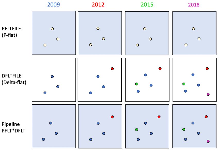
The calwf3 software selects the appropriate flat fields for calibration based on keywords
(DETECTOR, CCDAMP, FILTER, and DATE-OBS) in the header of each raw image. Sub-array
science frames use the same set of reference files as full-frame images, and calwf3 extracts the
appropriate region of the detector from each flat field.

Until now, only the PFLTFILE has been used in the pipeline, first in 2008 when the ground P-flats
were delivered, and again in 2010 when a smoothed ‘grey’ correction was applied to the P-flats.
In our study, six filters (F0098M, F105W, F110W, F125W, F140W, and F160W) have sufficient
signal-to-noise that the flats are now derived purely from in-flight data and are no longer dependent
on the ground test data. For the remaining nine IR filters, the ground P-flats were multiplied by a
smooth correction derived from wavelength-interpolation using sensitivity residuals from the six
‘primary’ filters.

In the past, low-order flat corrections have been computed for both WFC3 detectors, but these
have never been carried as a separate LFLTFILE reference file. For the UVIS detector, low-
frequency corrections to the ground P-flats derived from dithered star cluster data were applied
directly to the P-flats, and a modified version of the PFLTFILE was delivered (Mack et al. 2013).
Similarly for the IR detector, a smooth ‘grey’ correction was applied to the ground P-flats in the
P2011 PFLTFILE delivery. Pirzkal et al. (2011) referred to the ‘grey’ correction as a ‘sky-delta’
or SD-flat since it provided a correction to the P-flat, albeit smoothed to correct for noise.

In this work, we use the term ‘delta-flat’ strictly to describe high-spatial frequency corrections to
the P-flat. In coordination with this analysis, Olszewski & Mack (2021, in prep.) make use of the
‘available’ but previously unused DFLTFILE reference file. To correct for low-sensitivity IR
‘blobs’ appearing over time on the Channel Select Mechanism (CSM), the authors create a set of
49 D-flats for each of the six primary filters, corresponding to each unique ‘date of appearance’.
Figure 1 shows how the PFLTFILE and DFLTFILE are combined by calwf3 during the
FLATCORR step. While there is only one set of P-flats for all dates (row 1), the D-flats (row 2)
have unique USEAFTER dates corresponding to the appearance of new blobs. The DATE-OBS
keyword for each input exposure is used to select the appropriate flat field USEAFTER date.
Sunnquist (2018) lists all known blobs, their epoch of first appearance, coordinates, radius, and
“flux” (a colloquialism for the equivalent width of the absorption of the blob.)

 For ‘early’ appearing blobs, either in ground test data or in early in-flight data, sky flats will have
little to no signal in the affected pixels. We therefore replaced pixel values in the P-flats
corresponding to blobs 1-29 (through September 2009) with the median value from the P-flat in a
circular annulus 20 pixels in width surrounding each blob. This was also done for an additional 46
blobs which were discovered in the ground flat images by blinking the blob masks with the flat
field error arrays. These 46 blobs were improperly marked by Sunnquist as appearing on July 25,
2010, which is the first time they were seen in Earth flat observations due to being very faint.
More detail on the treatment of IR blobs is provided in Olszewski & Mack (2021, in prep.)

 4

In Figure 1 (top row), ‘early’ blobs in the PFLTFILE are shown as yellow circles. While these
affect all IR observations, they were kept separate from the P-flats to make the later more useful
for IR grism calibration. Pirzkal & Ryan (2020) used a nearly final version of these P-flats in their
analysis of the dispersed IR sky background for G102 and G141. Blobs show up in the Zodiacal
light component as elongated shapes, similar to those of normal dispersed spectra but with lower
signal due to the reduced sensitivity. The blobs are also apparent in the Helium I component, but
they are offset from their nominal positions in imaging data due to the grisms’ dispersion.

The second row of Figure 1 shows the contents of four hypothetical D-flats, where the left-most
column shows the pixel-to-pixel sensitivity for all ‘early’ blobs which were replaced with a
constant value in the P-flat. Blob values in the DFLTFILE are normalized (divided) by the same
constant value, and this cancels out when calwf3 multiplies the P-flat and the D-flat. New D-flats
are provided for each unique blob appearance date, and calwf3 uses the USEAFTER date to select
the appropriate reference file for calibration.

Figure 1: An illustration of the PFLTFILE and DFLTFILE reference files for a single IR filter.
The same P-flat is used for all USEAFTER dates, indicated by the 4 columns. In the top row, light
blue regions show the pixel-to-pixel correction and yellow circles show ‘early’ blobs which were
filled with a constant value from an adjacent region of the P-flat. The middle row shows four
hypothetical D-flats containing an increasing number of blobs, indicated by the colors (blue, red,
green, and purple) corresponding to each epoch (2009, 2012, 2015, 2018). Regions of the flat
outside the blobs are filled with a value of 1.0. The two flat field reference files are multiplied
together by calwf3 to create the combined flat in the bottom row.

 5

III. Observations
The ideal datasets for creating sky flats are sparse fields with a high, spatially uniform background.
The background is primarily a combination of zodiacal light and Earthshine at shorter
wavelengths, and telescope thermal emission at longer wavelengths (Dressel 2018). The F105W
and F110W may contain additional background from Helium I airglow at 1.083 microns, typically
strongest at low Earth limb angles outside the Earth’s shadow. In the worst cases, this line strongly
dominates the total background (Brammer et al. 2014). We used many datasets with Helium
emission for this study, but they were first corrected for time-variable background prior to the
ramp-fitting step in calwf3. Exposures with both time- and spatially varying background due to
scattered light from the Earth’s limb were also included, but the impacted reads were masked prior
to running calwf3. This process is described in more detail in the Appendix.

The same set of 30 programs used for the P2011 sky flats (~1900 datasets through 2010) were
used for this analysis, except for programs 11650 (UVIS only) and 11644 (F139M, F153M only).
Additional archival datasets were identified by a MAST search with fields: Apertures= ‘IR*’,
Exptime= ‘>300’, Filter= ‘F*’ (no grisms), Keyword= ‘High redshift galaxy’, ‘High redshift
cluster’, ‘Blank*’, or ‘High latitude field’. Only exposures with NSAMP > 5 were selected to
insure that calwf3 will reliably produce an accurate ramp fit.

Table 2 lists the 134 program IDs, which includes over 14,000 FLT images observed between July
2009 and December 2019. For galaxy cluster studies, eg. CLASH (12065, 12068, 12451, 12453,
12460) and Frontier Fields (13495, 13496, 13498, 13504, 14037, 14038), only parallel
observations were selected in order to avoid spatial variations in the background due to intracluster
light. Other large surveys in our data sample include: CANDELS, (12064, 12440, 12442, 12443,
12444, 12445), 3DHST (12177, 12328), WISP (13352, 13517, 14178), HUDF-DEEP (11563,
12498), and HIPPIES (12286).

Table 2: GO programs used for the sky flat analysis, including data from 134 programs observed
between July 2009 and Dec 2019. Programs IDs used for the P2011 flats are shown in red.

 11108 11142 11149 11153 11166 11189 11202 11208 11343 11359
 11439 11519 11520 11528 11534 11541 11557 11563 11584 11587
 11597 11600 11602 11624 11636 11663 11666 11669 11694 11696
 11700 11702 11709 11734 11735 11738 11838 11840 12005 12025
 12051 12060 12061 12062 12063 12064 12065 12068 12099 12167
 12177 12184 12194 12203 12224 12247 12265 12283 12286 12307
 12328 12329 12440 12442 12443 12444 12445 12451 12453 12460
 12471 12487 12496 12498 12572 12578 12581 12616 12764 12766
 12905 12930 12942 12949 12959 12960 12974 12990 13000 13002
 13045 13110 13117 13294 13303 13352 13480 13495 13496 13498
 13504 13517 13614 13641 13644 13677 13688 13718 13767 13792
 13793 13831 13844 13868 13951 14037 14038 14178 14262 14327
 14459 14699 14718 14719 14721 15118 15137 15212 15242 15287
 15436 15644 15697 15702

 6

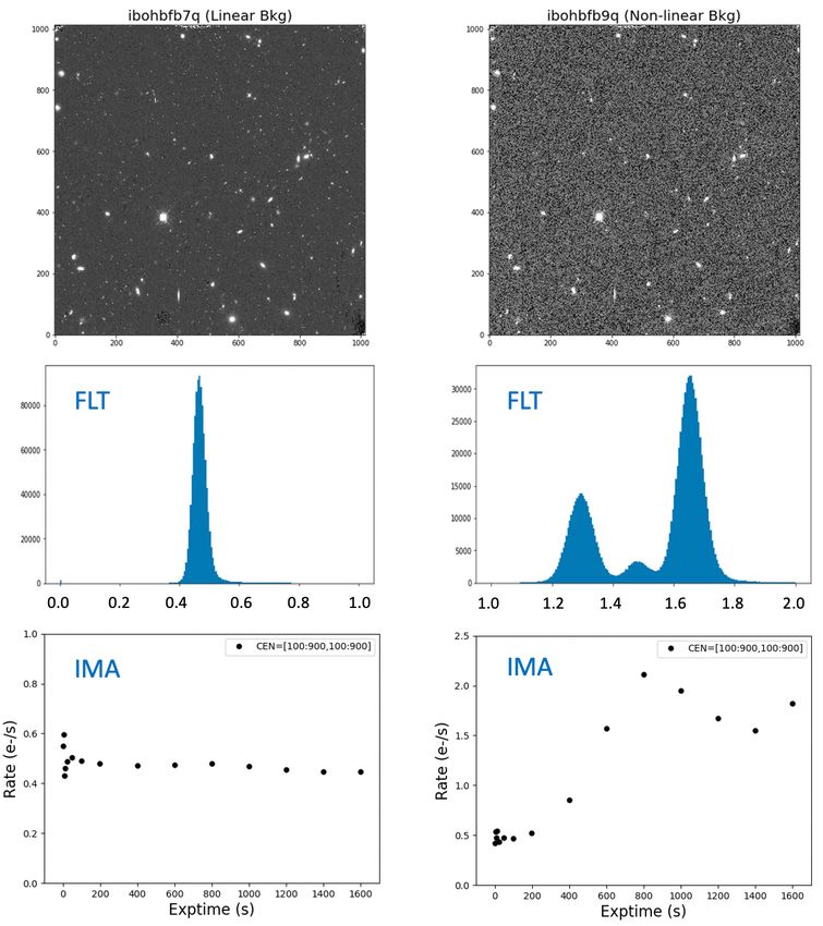
Table 3: The archival data sample used to compute sky flats. Column 2 lists the mean background
(e-/s/pix) from the images this study, which may be compared to three background estimates
derived using ETC v28.2 in column 3. The three ETC values correspond to: 1) ‘AvgZodi’, 2)
‘AvgZodi+AvgEarthshine’, 3) ‘AvgZodi+AvgEarthshine+Thermal+Dark’. Columns 4-8 give the
maximum possible and mean number of FLT frames in each sky flat, the maximum exposure time
in units of 106 seconds, the mean signal in units of 106 electrons/pixel, and the corresponding
Poisson-limited estimate of the mean error in percent. Statistics are provided only for the six filters
with sufficient data to replace the ground flats, which had errors ~0.2%.

 P-flat Mean ETC Max Mean Max Mean Mean
 Filter Sky Background Number Number Exposure Signal Error
 -
 . (e /s/pix) (1, 2, 3) of FLT of FLT (106 sec) (106 e-/pix) %

 F098M 0.4 ± 0.2 0.44, 0.57, 0.67 737 380 0.7 0.17 0.24%

 F105W 1.0 ± 0.5 0.77, 1.00, 1.11 1875 1070 1.8 1.00 0.10%

 F110W 1.7 ± 1.0 1.30, 1.70, 1.79 679 370 0.4 0.33 0.17%

 F125W 0.8 ± 0.4 0.77, 0.99, 1.09 3167 1600 2.1 0.86 0.11%

 F140W 1.0 ± 0.5 0.95, 1.21, 1.33 1385 680 0.9 0.47 0.15%

 F160W 0.7 ± 0.3 0.59, 0.75, 0.93 5550 2870 4.0 1.39 0.08%

In Table 3, we report the mean sky (e-/s/pix) for each filter in our sample with the corresponding
1-sigma standard deviation. We compare this with three background predictions from the ETC,
described in the table caption. Sky values determined from FLT images were computed after
masking sources and correcting the data for varying background. For these six IR filters, the ETC1
prediction ranges from 0.4 e-/s/pixel in F098M to 1.3 e-/s/pixel in F110W. To achieve a minimum
signal-to-noise (S/N) of 10 at the lowest background, we limited our data sample to include only
exposures longer than 300 seconds. By contrast, the largest sky background in our sample was a
1600 second exposure in F105W with a sky background of 3.0 e-/s/pixel, yielding a S/N of ~70.

In columns 4 and 5, we list the maximum number of FLT frames to be combined in each filter and
the mean number of FLT frames per pixel in the combined stack (after masking sources). In
general, the mean is approximately half the total number of frames, similar to the results presented
in Pirzkal et al. (2011). This is because approximately half of all detector pixels in a given FLT
are masked prior to stacking, as described in Section 4. The maximum total exposure (in million
seconds) in column 6 corresponds to the sum of the individual exposure times, without any
masking. This means that simply multiplying the mean sky by the maximum exposure time gives

 7

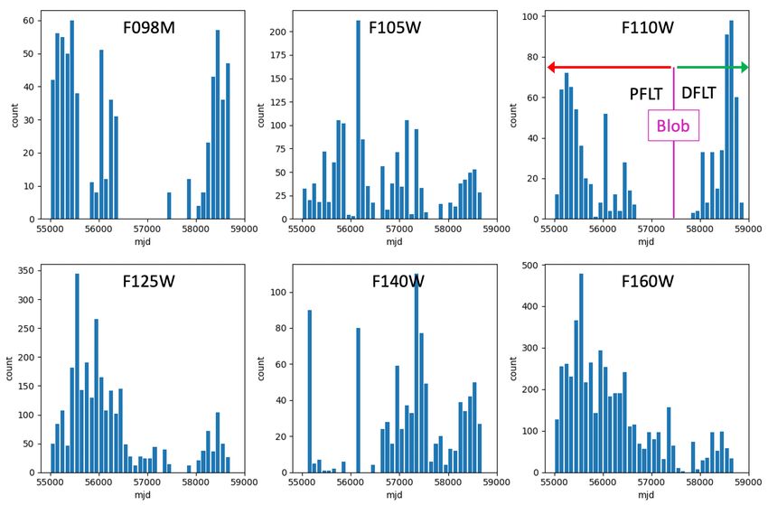
a total possible signal value which is approximately twice the mean signal per pixel (in million
electrons) reported in column 7.

In column 8, we give the mean error per filter (in percent) based on Poisson statistics. Assuming a
mean sky background ~1.0 e-/s and a mean exposure of 700 seconds, a stack of 340 frames per
pixel would be required to match the ~0.2% error (S/N ~500) in the ground P-flats. Sky flats
derived for the six filter in this study range from a S/N ~400 in F098M to S/N ~1200 in F160W.
For comparison, the P2011 flats had average S/N ~700 for the ‘grey’ correction, with individual
filters ranging from S/N ~140 in F140W to S/N ~500 in F160W.

In Figure 2, we plot a histogram of the number of IR images in our archival data sample for each
filter as a function of date (MJD). For regions on the detector which are free from blobs, the entire
set of FLT images was stacked in order to generate the P-flat (sky flat). For regions impacted by
blobs, only observations acquired before the blob appeared were used to derive the P-flat, while
only observations after the blob appeared were used to derive the D-flat. Note that flats were
computed only for blobs with sufficient in-flight data such that Poisson errors are below 1%. This
excludes any ‘recent’ blobs which appeared after July 10, 2018 (Olszewski & Mack, 2021 in prep).
Sky flats were computed for six IR filters with sufficient signal-to-noise to replace the ground flats.
Improvements to the P-flats for an additional nine IR filters are discussed in Section 7.

Figure 2: Histogram showing the number of IR datasets in the sky flat sample for six filters as a
function of date (MJD) in bins of 100 days. Data acquired before a blob appears can be used to
derive the P-Flat, and data acquired after a blob appears can be used to make the Delta-Flat. This
is illustrated for the F110W filter for a hypothetical blob first appearing at MJD 57500.

 8

IV. Analysis
To compute the sky flats, we apply several corrections to optimize the calibrated FLT data products
prior to stacking the data, including the use of custom bad pixel masks, masking persistence from
prior observations, correcting for time-variable background, and improving the linear ramp fit
performed by calwf3. The full procedure is detailed in the steps below, which highlights the
identifcation and masking of sources, stray light, and detector artifacts.

1.) Recalibrate each RAW file with updated IR darks (Sunnquist et al. 2019) and custom bad pixel
tables (BPIXTABs) which contain time-dependent masks for both strong and weak blobs (as
classified by Sunnquist 2018). Currently, the BPIXTABs only contain DQ flags for strong blobs.

2.) As part of the recalibration, we use the P2011 flats (u*pfl.fits) so that the FLT data products
have nearly uniform background across the detector. This allows us to use a constant signal-to-
noise ‘threshold’ for detecting sources across the entire image (see step 7). The 2008 ground flats
(s*pfl.fits) were not used, as they introduce spatial residuals in the background resembling a cross
pattern caused by the stimulus support structure. Once the source masks have been generated, the
RAW data are later recalibrated with the flat field correction turned off (see step 9).

3.) Identify reads in the IMA contaminated by scattered light from the Earth limb which introduce
a spatially variable background. Rerun calwf3, excluding those reads, to improve the ramp fitting
(CRCORR) step. This process is described in more detail in the Appendix. In short, if the ratio of
the sky background on the LHS/RHS of the detector is greater than 1.05, the read is flagged and
rejected. This results in a slightly shorter FLT exposure and a flat background across the detector.
In the P2011 flats, FLT images with scattered light were excluded when the mode and median of
the background were different by more than 5%. While this method is effective in removing
contaminated datasets, it rejects the entire FLT dataset instead of just the impacted reads.

4.) Correct for time-variable background due to Helium I emission from the Earth’s atmosphere in
the F105W and F110W filters. This background does not vary spatially, so the correction is
performed by subtracting the median background from each read of the IMA and rerunning the
ramp fit in calwf3. We then added back a constant value representing the average count rate of the
full exposure to preserve pixel statistics. This is described in more detail in the Appendix and is
based on methodology by Brammer (2016) which works well for sparse fields where the sky
background may be accurately computed.

5) In the recalibrated FLT data, mask bad pixels with data quality (DQ) flags 4, 8, 32 (bad detector
pixel, signal in zero read, unstable response) by setting their value to ‘nan’ in the science array.
Keep any pixels flagged 16, which are now classified as ‘stable’ hot pixels and which are corrected
during the DARKCORR step when calwf3 applies the latest IR dark reference files. Mask both
strong and weak blobs in the science array which are flagged as 512 in the DQ array.

6.) Using persistence models provided by MAST, mask any residual signal in the science array
from IR observations acquired up to 16 hours prior. The latest model is a spatially-averaged

 9

‘A-gamma model’ based on the exposure time and fluence level in the stimulus exposure and
allows for different regions of the detector to have different power law decays (Long et al. 2018).
Pixels in the model image (‘*_persist.fits’) with values greater than 0.005 e-/s were used to mask
pixels in the science array of each FLT. This is the same threshold used to mask pixels in the HST
Frontier Fields data pipeline (Koekemoer et al. 2020). The IR dark rate is 0.05 e-/s, so this threshold
is ~10x fainter due to the need to stack many frames to derive a high signal-to-noise sky flat. For
the P2011 flats, these models were not yet available, so persistence was masked by identifying
‘any pixel that was filled by more than 30,000 e- in any exposure taken within three days prior’.

7.) Identify sources using image segmentation tools implemented in ‘photutils’. The function
‘detect_threshold’ produces a 2D detection threshold image using sigma-clipped statistics to
estimate the background level and RMS. Prior to detecting sources, we first smooth the data using
the ‘astropy.convolution’ function ‘Gaussian2DKernel, a 2-dimensional circular Gaussian kernel
with a FWHM ‘sigma’ of 1.5 pixels and a size of 3 pixels in both x and y. Smoothing maximizes
the detectability of objects with a shape simiar to the filter kernel. Sources with a minimum of 4
connected pixels above a threshold of 0.75 sigma over the background were selected for the
segmentation image. (For the P2011 flats, source masks were computed using SExtractor with a
threshold value of 0.85 sigma and 4 connected pixels.) We create an object mask by setting all
non-zero pixels to 1 and leaving the remaining ‘sky’ pixels set to zero.

8.) Exclude the edges of very faint sources which are below the detection threshold. To achieve
this, we grew the segmentation mask from step 7 by convolving with a 2D circular Gaussian kernel
with σ=7 pixels using the ‘astropy.convolution’ task ‘convolve’. Finally, we set any values less
than 0.012 in the convolved image to zero and all other values to 1. This cutoff value was
determined empirically from visual inspection of the data products, as a compromise between
masking the faint wings of astronomical sources, but not masking too many pixels in the image.
For the P2011 sky flats, segmentation masks were convolved with a Gaussian kernal with σ=10
pixels and a cutoff value of 0.03. Both methods effectively expand the mask of a point source to a
diameter of 40 pixels.

9.) Recalibrate the RAW frames a final time, but with the flat field correction set to OMIT. During
the final recalibration, exclude reads contaminated by scattered Earth light identified in step 3, and
rerun the time-variable Helium I background correction described in step 4.

10.) Reapply the bad pixel masks for DQ flags 4, 8, 32, 512 to the FLT science array, as described
in step 5. Reapply the persistence masks from step 6 and the object masks from steps 7 and 8.

11.) Normalize each FLT image by dividing by the median value of the remaining (sky) pixels in
the region [101:900,101:900], recommended by Bushhouse (2008). This region avoids detector
defects such as the Death star, wagon wheel, unbonded pixels, etc.

12.) Exclude FLT images with any residual unmasked signal. To identify these, we computed the
ratio of the mean to the median sky background and sorted the list in descending order by the ratio
value. Examining each image, we selected a cutoff value (ratio > 1.0011) to identify datasets with
obvious problems. We also excluded any FLT images with more than 75% of detector pixels

 10

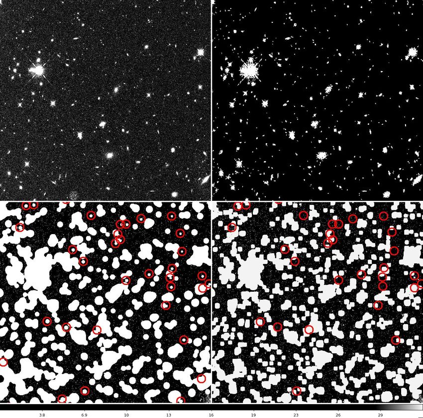
masked. These two criteria allowed us to discover a handful of anomalies, including trailed sources
caused by pointing errors, unmasked diffraction spikes, the faint wings of bright stars or extended
galaxies, persistence not captured in the models, or scattered light from the Earth limb which
appeared in many reads. With these additional checks, ~5% of the FLT images were excluded
from our data sample.

Figure 3: F160W calibrated image: ‘ibhg05zcq_flt.fits’. Starting with the original FLT data (UL),
we create a segmentation map (UR), which is then Gaussian-smoothed and added to the DQ mask
(LL). For comparison, we show the mask from the P2011 analysis (LR) which looks very similar
to the mask from this study. Red circles indicate the position of the blob masks. These were not
masked in the P2011 flat analysis and are therefore dark in this figure (LR), except where they
coincide with sources in the object mask.

 11

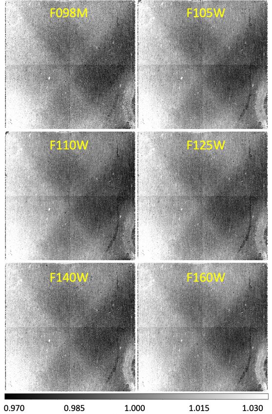
In Figure 3, we compare masks generated for an example FLT image from this work using
‘photutils’ and from the P2011 flat analysis which used SExtractor. Parameters in this work were
fine-tuned to achieve similar results to the prior study, albeit with somewhat more aggressive
masking in the wings of sources which is possible because of our larger data sample. We notice
that our object masks are slightly less ‘blocky’ than the P2011 masks, and this is more
representative the true shape of astronomical sources in these images. In the example FLT image,
54% of all detector pixels were good (unmasked) using the analysis described in this report,
whereas 63% were good using the P2011 analysis.

For the images in our data sample, anywhere between 25% and 80% of pixels in a given image are
good (unmasked), with a mean value of 45%. While this means that a large fraction of the detector
is masked in each image, the random distribution of sources on the sky, combined with a large
number of independent datasets results in fairly uniform spatial coverage over the array.

V. Results

After masking sources and bad pixels, we stacked the images in each filter by computing the mean,
the median, and the signal-weighted average of the normalized FLT frames. These combined
stacks are the basis of the new P-flat reference files. We find that the signal-weighted average
tends to give higher weight to images with scattered light residuals at the curved, right edge of the
Earth limb feature which changes position slightly throughout the exposure. While the rms in the
background is overall the lowest in the weighted average, the resulting P-flat shows systematic
spatial residuals in the background compared to the other two methods. We find that the mean
stack has a much larger rms than the median stack, possibly due to hot or unstable pixels which
were not flagged in the DQ arrays.

Pixels classified as detector artifacts (DQ flags=4, 8, 32) were masked in every FLT frame, so the
sky flat is undefined in these regions. Rather than leave holes in the P-flat, these pixels were filled
with sensitivity values from the P2011 pipeline flat. Typically, these bad pixels are rejected when
combining dithered observations, so this choice of fill value is primarily helpful in producing
cosmetically ‘clean’ FLT images.

In Figure 4, we show wavelength-dependent residuals with respect to the prior set of P-flats, i.e.
the ratio of the new sky flats to the P2011 flats. These six panels reveal features in a given filter
which were not corrected by the prior ‘grey’ inflight correction. For the central 800x800 region of
the detector, we find residuals of ± 0.5%, strongest in the F110W filter and correlated with the
cross pattern in the ground flat, and weakest in the F160W filter, presumably because about half
of the data used to derive the P2011 ‘grey’ correction was in F160W.

Curiously, the wagon wheel, a curved region in the lower-right of the detector with reduced
sensitivity, shows the largest residuals (up to ~2%) in F160W and F140W but almost no residuals
in F098M and F110W. We hypothesize (but have not confirmed) that sigma-clipping may have
rejected these residuals when combining images from all six filters to create the P2011 ‘grey’ flat.

 12

Figure 4: Correction to the P2011 flats for 6 filters, showing wavelength-dependent residuals with
respect to the ‘grey’ correction of ±0.5% in the central 800x800 region of the detector and up to
2% in the lower right corner. White circular features are smoothed blobs in the P2011 flats.

 13

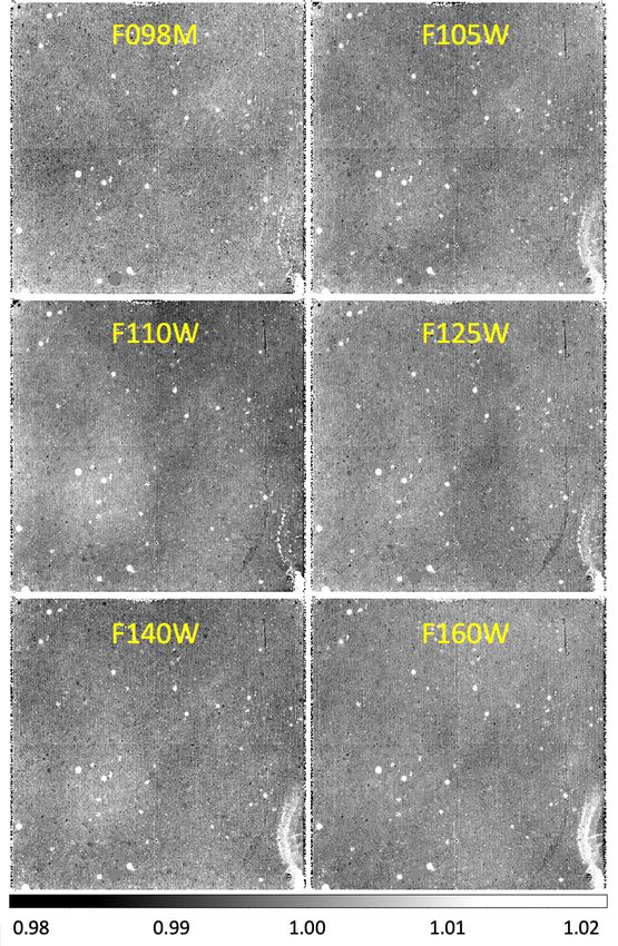
Figure 5: Correction to the ground P-flats for 6 filters. Most notable is a large cross pattern in the
ground flats caused by the optical stimulus support structure. White circular features are caused
by blobs that existed in the ground flats but whose position shifted due to the in-flight optical
alignment.

 14

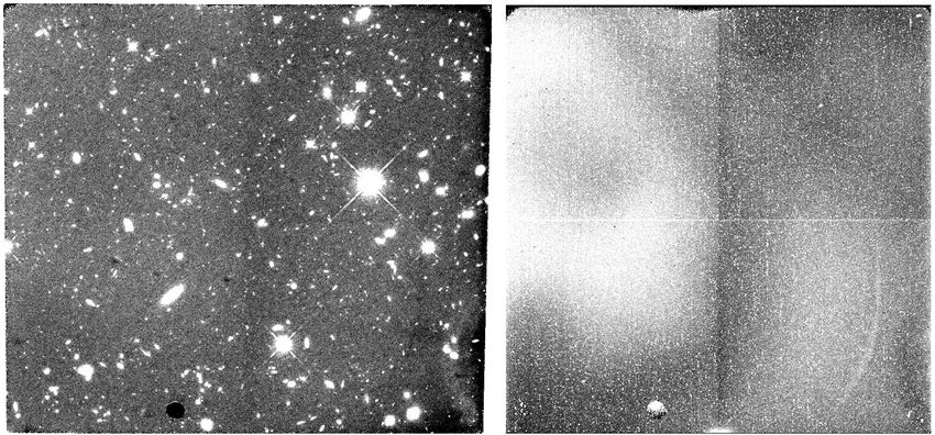
IR blobs which were present in images acquired through 2010 were not masked when computing
the P2011 flats, and these appear as compact, white features in the Figure 4 sensitivity residuals.
Because the prior analysis did not include these time-dependent masks, any new blobs which
appeared in-flight were stacked together with data before the blob appeared, reducing the overall
strength of the blob. Additionally, the ‘grey’ flat correction was smoothed to reduce noise using
Fourier filtering with σ=10 pixels (Pirzkal et al. 2011). Therefore, blobs in the ‘grey’ flat are
slightly larger than their actual size. Smoothing also affected pixel-to-pixel features in the P-flat,
making them both larger in size and reduced in strength. Those features appear in Figure 4 as dark
residuals surrounded by a white ring. For example, a cluster of bad pixels (DQ=4) at detector
position x,y ~ (500, 170) increased in radius from ~2 pixels to ~4 pixels in radius after smoothing.

Figure 5 shows the sensitivity residuals with respect to the ground flat, e.g. the ratio of the sky flat
and the original ground P-flat. In this view, the cross-pattern due to the stimulus support structure
used for the ground test is most noticeable and dominates any wavelength-dependent features seen
in Figure 4. White features show blobs which were present in the ground flats but which shifted
position to the left by ~20 pixels and downward by ~10 pixels after the in-flight alignment.

VI. Improvement in DRC products

To demonstrate the improvement in MAST drizzled products calibrated with the new flat fields,
we selected observations from our archival data sample with a large sky background. In Table 4,
we provide the association name for three broadband filters, the number of FLT frames in the
combined DRC drizzled image, the combined exposure time, and the total sky in units of 103
electrons per pixel. We also list the number of blobs appearing at the date of observation.

In last two columns, we compare the rms of the sky background (iteratively clipping pixel values
deviating by more than 5-sigma after 10 iterations) measured in the prior (2011) and in the new
(2020) drizzled data products. These images are displayed in Figures 6-8, and in all three cases,
the images are visually improved when using the new flats and the rms of the background is
reduced. Olszewski et al. (2020) present blinking GIF images in their electronic AAS poster
comparing the old and new drizzled data products, making it easier to visualize the improvement
in the background. (We provide a link to the poster in the References section of this report.)

Table 4: Visit-level DRC products from MAST used to test the new PFLT*DFLT calibration.

 Filter Dataset ID N Exptime Total Bkg Date # RMS RMS
 (sec) (103 e-/pix) Blobs 2011 2020
 F105W IBOHBH020 6 9,595 14.1 2013-01-07 123 0.0147 0.0135
 F125W IA2101010 8 10,423 24.8 2010-10-16 106 0.0191 0.0171
 F140W IBKDF2010 4 5,212 10.4 2013-07-10 127 0.0201 0.0185

 15

Figure 6: F105W dataset ‘ibohbh020_drz.fits’ with a total background of 14,100 electrons
calibrated with the prior flats (top) and with the updated flats (bottom).

 16

Figure 7: F125W dataset ‘ia2101010_drz.fits’ with a total background of 24,800 electrons
calibrated with the prior flats (top) and with the updated flats (bottom).

 17

Figure 8: F140W dataset ‘ibkdf2010_drz.fits’ with a total background of 10,400 electrons
calibrated with the prior flats (top) and with the updated flats (bottom).

 18

For the F105W and F140W example datasets, the blobs are completely removed via flat fielding,
whereas for F125W, they are only partially removed. This is because the blobs lie on the WFC3
Channel Select Mechanism (CSM) which does not always return to the same nominal position
(McCullough et al. 2014). The blob flats represent the average over a range of CSM angle
positions, and any given dataset may show mis-registration of the blobs caused by offsets in the
CSM position. Olszewski & Mack (2021, in prep.) discuss future work to derive a set of blob flats
corresponding to a range of possible CSM positions.

Some datasets still show low-level residuals ~0.005 e-/s in the background, and these structures
are similar in shape to the IR dark. In Figure 9, we compare the improved F125W drizzled image
from Figure 7 with the SPARS100 dark reference file used for the calibration. Nominal variations
in the mean dark current reported by Sunnquist et al. (2017) may be as large as ± 0.007 e-/s for a
mean rate of 0.049 e-/s. This suggests that users may further improve the uniformity of calibrated
FLT data by removing any fluctuations in the IR dark current prior to applying the flat field.
Instead of rerunning calwf3, this may be achieved by subtracting an appropriately scaled version
of the dark divided by the P-flat from each FLT image to best flatten each background prior to
drizzling.

Figure 9: (Left) The improved F125W drizzled product ‘ia2101010_drz.fits’ from Figure 7 shows
low-level residuals at the midline of the detector ~0.005 e-/s. This is consistent with nominal
variations in mean dark rate of 0.049 e-/s ± 0.007 e/s. (Right): The SPARS100 dark used for
calibration shows structure similar to the background residuals seen in the drizzled image.

 19

VII. L-flats for Other Filters

For the remaining nine IR imaging filters, we used the wavelength-dependent sensitivity residuals
from the six ‘primary’ filters to correct the P-flats acquired on the ground. These residuals were
later smoothed (as described below) to avoid degrading the filter-dependent pixel-to-pixel
sensitivity and are therefore referred to in this section as L-flats.

The L-flat correction ‘L’ for each filter was derived by first interpolating the pixel values of the
flat field residual images (sky flat divided by ground flat) L1 and L2 from the two filters closest
in wavelength:

 ( – ) ( ' )
 = ∗ + ∗ 
 ( ' ) ( ' )

where λ is the pivot wavelength of the interpolated filter, λ1 is the pivot wavelength of the nearest
‘blue’ filter with L-flat L1, and λ2 is the pivot wavelength of the nearest ‘red’ filter with L-flat L2.

The interpolation fraction for each filter is listed in the third column of Table 5. For F126N,
F127M, F128N, F130N, and F132N, the L-flat was computed from appropriate linear
combinations of the F125W and F140W L-flat. Because the F139M filter is so close in wavelength
to F140M, we simply used the F140W L-flat rather than interpolating. This was also done for
F153M which is very similar in wavelength to F160W. There is no broadband filter redder than
F160W, so the F164N and F167N filters also used the F160W L-flat.

Since is not yet possible to compute blob flats for these nine filters, we opted to include ‘early’
blobs as part of the filter-dependent L-flat. For example, to compute the F140W L-flat, we
multiplied the sky P-flat times the D-flat from November 25, 2009 (which includes blob IDs #1-
33) and then divided by the ground P-flat. While Sunnquist (2018) cataloged only 24 blobs in early
in-flight observations (as of July 31, 2009), we decided to include nine additional blobs in this
‘early’ set. These include three of the strongest blobs observed to date (IDs #25, 27, 33) and affect
most IR observations. We also include 46 faint blobs which were first noticed in Earth flat
calibration observations acquired on July 25, 2010 but which we traced to the original ground flats.
While these blobs were not apparent in the flats themselves, they are easily identifiable as blob
pairs in the flat field error arrays. This is because of a realignment which was done in the middle
of the IR ground flat calibration campaign, so a single blob shows up as a pair of slightly offset
blobs with Ö2 larger errors than the surrounding regions of the P-flat.

We flagged both strong and weak blobs in the D-flat data quality (DQ) array for the six filters with
sky flat solutions. For all other filters, the 33 + 46 = 79 ‘early blobs’ were incorporated directly
into the P-flats and are therefore flagged in the DQ array of the PFLTFILE reference file. The flat
fielding in the blob regions will not be perfect, so these flags (DQ value = 512) will allow users to
easily reject affected pixels when combining observations acquired using the ‘IR-BLOB-
DITHER’ pattern.

 20

Finally, we smoothed the L-flat correction for each filter using a circular median filter of radius 5
pixels with lower and upper rejection thresholds of 0.8 and 1.1, respectively, corresponding to the
typical range of flat field values. We then multiplied the smoothed L-flat by the original ground
P-flat for these nine filters to produce a revised set of PFLTFILE reference files. (We note here
that a similar methodology was used for computing L-flats for the UVIS detector for filters with
no dithered star cluster observations, cf. Mack et al. 2013.)

The sky background is typically very low in these other nine medium- and narrow-band IR filters,
so the improvement in calibrated data is barely noticeable when using the new P-flats. For
example, a 6130 second drizzled image ‘ibwjcd040_drz.fits’ from program 12461 acquired in the
F153M filter contained only 600 electrons of sky background, corresponding to a count rate of
~0.1 e-/s.

Table 5. The 15 WFC3/IR filters and their corresponding pivot wavelength. Filters with
insufficient data to directly derive a sky flat are indicated in blue font. For those, the correction to
the ground flats was based on L-flat solutions from filters close in wavelength (black font) and is
interpolated using the pivot wavelength of the filter, as shown in column 3. For filters where the
correction is primarily from a single filter (e.g., F139M and F153M), the nearest broadband filter
solution is used rather than the interpolated solution, as indicated in column 4. For the two reddest
narrow filters, the F160W solution was used. The name of the updated P-flat reference files are
listed in column 5 for each filter.

 Filter Pivot Interpolation Formula L-flat P-Flat
 Wave Used Reference File
 (A)
 F098M 9865 4ac1921gi_pfl.fits
 F105W 10551 4ac1921ii_pfl.fits
 F110W 11535 4ac1921ji_pfl.fits
 F125W 12486 4ac1921li_pfl.fits
 F126N 12585 0.93 * F125W + 0.07 * F140W 4ac1921ni_pfl.fits
 F127M 12704 0.82 * F125W + 0.18 * F140W 4ac1921oi_pfl.fits
 F128N 12832 0.76 * F125W + 0.24 * F140W 4ac1921qi_pfl.fits
 F130N 13006 0.64 * F125W + 0.36 * F140W 4ac1921ri_pfl.fits
 F132N 13188 0.51 * F125W + 0.49 * F140W 4ac1921ti_pfl.fits
 F139M 13838 0.06 * F125W + 0.94 * F140W F140W 4ac19221i_pfl.fits
 F140W 13923 4ac19222i_pfl.fits
 F153M 15322 0.03 * F140W + 0.97 * F160W F160W 4ac19224i_pfl.fits
 F160W 15369 4ac19225i_pfl.fits
 F164N 16404 F160W 4ac19227i_pfl.fits
 F167N 16642 F160W 4ac19228i_pfl.fits

 21

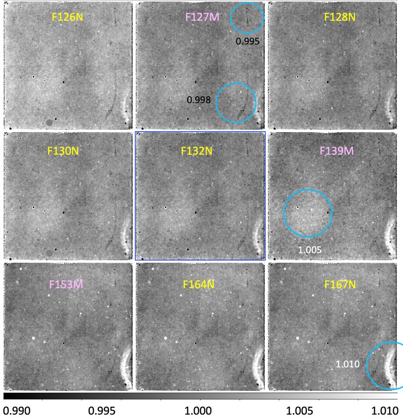
Figure 10 shows the smoothed L-flat correction for the nine IR filters with respect to the P2011
flat. While the L-flat residual is actually computed with respect to the ground P-flat, we elected to
show the residuals with respect to the P2011 flat because the total correction is smaller, making it
easier to see wavelength-dependent residuals. Note that the F167N correction in the lower-right
panel is identical to the F160W residual shown in Figure 4, except for additional smoothing which
reduces the strength of the ‘wagon wheel’ residual slightly from 2% to 1% in the lower-right corner
of the detector. Because the blobs were included in the P-flats, the residuals in these regions are
also unique and reflect the color-dependence of the blobs.

Figure 10: Wavelength-dependent residuals with respect to the P2011 flats for the 9 filters with
no sky flat solutions, displayed with a scale from 0.99 to 1.01. Medium-band filters are shown in
pink font and narrow-band filters in yellow font. Regions with the largest sensitivity residuals are
circled in blue. These include the ‘scar’, a dark narrow region with residuals up to 0.995 in F127M
and the wagon wheel, a bright curved region at the lower-right with residuals up to 1.010 in F167N.

 22

Olszewski & Mack (2021, in prep.) report that the blobs absorb light more in bluer filters,
compared to F160W where they are the weakest. In the top two rows of Figure 10, blobs show
dark residuals in their centers, indicating that they are stronger in the new P-flats compared to the
P2011 flats. This makes sense since the P2011 flats were heavily weighted to images in the F160W
filter. Outside of their dark centers, the blobs show a ring of white residuals surrounding each blob
where they were ‘smoothed’ in the P2011 solution and therefore made larger. Residuals for the
three filters in the bottom panel are identical and are based on the F160W L-flat. These show
primarily white residuals in the blob regions, indicating that they are slightly less deep than they
were in P2011 flats. We attribute this to differences in the smoothing parameters between the two
studies.

VIII. Summary

New pixel-to-pixel P-flats were computed from deep images of the sky background in six IR filters.
For an additional five filters, the ground flats were corrected by interpolating the sky flat sensitivity
residual from the two filters closest in wavelength. For the remaining four filters, we substituted
the sky flat residual from the filter closest in wavelength. An updated set of reference files was
delivered on 15 October 2020, and observations retrieved from MAST after this date will include
the latest flat field calibration. Otherwise, the new reference files maybe obtained via the
‘Calibration Reference Data System’ (CRDS) at https://hst-crds.stsci.edu for users who wish to
manually recalibrate their observations. Instructions for manual recalibation are provided in the
WFC3 Data Handbook (Gennaro et al. 2018a).

The P-fields are intended to be used together with a new set of ‘delta’ D-flats to correct for IR
blobs as they appear over time. The new flat fields accompany an updated set of IR zeropoints
computed from observations of HST flux standards acquired over 11 years which were calibrated
using the new flats (Bajaj et al. 2020). The observed countrates are consistent to within ~1% with
the 2012 IR photometric calibration which was based on the P2011 flat fields. Changes in the
zeropoints are primarily due to an update to the CALSPEC white dwarf models and an increase in
the reference flux of Vega (Bohlin et al. 2019). This changed the zeropoint by

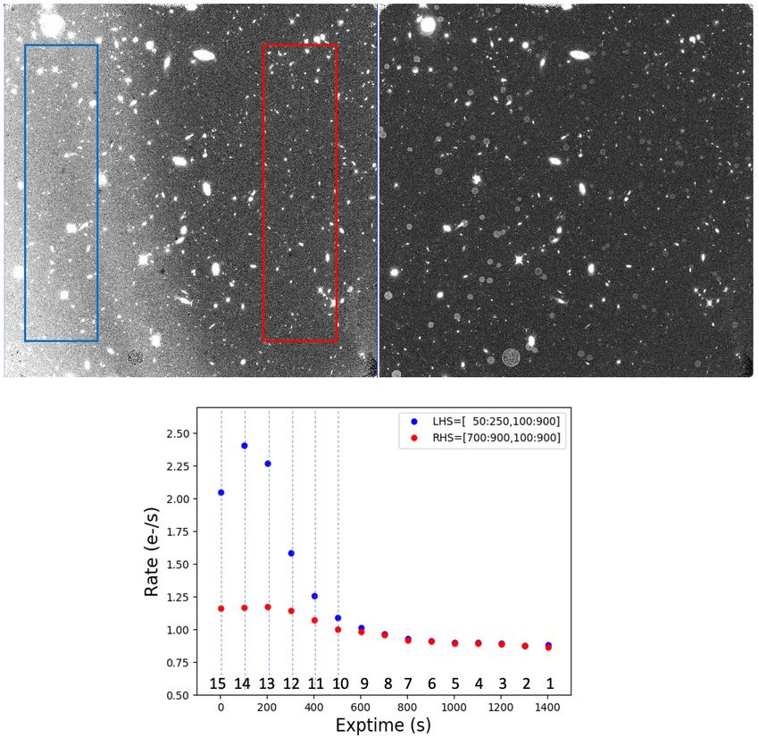
Appendix: Variable Background Correction

The quality of calibrated FLT data products for the IR detector depends on the accuracy of the
ramp fit performed by calwf3. Ramp fitting is performed during the ‘CRCORR’ cosmic-ray
rejection step of the pipeline. Any component of the IR sky background which varies with time
during an exposure will compromise the quality of the ramp fit and produce poor-quality calibrated
FLT images. Two components of the IR background which vary with time are: 1.) Helium I
airglow from the Earth’s atmosphere at 1.083 microns (affecting the F105W, F110W filters with
no spatial variation across the detector) and 2.) scattered light from the Earth’s limb (apparent in
any filter, with a strong spatial signature) appearing as an extended bright feature on the left side
of the IR detector. In this appendix, we describe the techniques used to improve FLT data which
were impacted by variable background, prior to including these in the sky flat analysis.

Helium I
To correct for time-varying Helium I emission, we followed the ‘Flatten-ramp’ method described
by Brammer (2016) to equalize the background signal rate for each F105W and F110W exposure
in our sample. Starting with the IMA file, we subtracted the median background from each read,
assuming a constant excess signal for every pixel. We then added back a constant value
representing the average count rate of the full exposure to preserve pixel statistics. We then resume
calwf3 processing to perform the ramp fit via the CRCORR step. Note that this approach works
well for relatively sparse fields where sky background is easily determined.

In Figure A1, we show two consecutive exposures in F110W (each with EXPTIME=1599.2
seconds, SAMP_SEQ= ‘STEP200’, NSAMP=16) comprising a single orbit of CANDELS
program 12442. The top-left panel shows the first exposure in the orbit ‘ibohbfb7q_flt.fits’ which
has a linear background rate over the entire exposure and a successful ramp fit. The center-left
panel shows a histogram of the sky background in the FLT image with the expected Gaussian
shape. The top-right panel shows the second image in the orbit ‘ibohbfb9q_flt.fits’ during which
the background rate increased significantly. The resulting FLT image is much noisier than
expected, and the sky background histogram (center,right) is not only broader than the first
exposure, but also strongly non-Gaussian and multi-modal.

In the bottom panel, we plot the average difference in the count rate between consecutive reads in
the IMA file using Equation 3 from Gennaro et al. (2018b), copied below.

The bottom-left panel of Figure A1 shows a roughly constant count rate per read of ~0.5 e-/s over
the entire exposure, whereas the bottom-right panel shows a background of 0.5 e-/s at the beginning
of the exposure, increasing rapidly to over 2.0 e-/s by the middle of the exposure. After correcting
for the time-dependent background, the sky in the recalibrated FLT is still larger than in the first
exposure but now shows the expected Gaussian distribution.

 24

Figure A1: (Top) Calibrated FLT data products for ‘ibohbfb7q_flt.fits’ and ‘ibohbfb9q_flt.fits’,
consecutive images of equal exposure time acquired in a single HST orbit. The left panel shows
the FLT resulting from a successful ramp fit, while the right panel shows the FLT from a poor
ramp fit due to time-varying background at the end of the orbit from Helium I emission in the
Earth’s atmosphere. This results in a noisy-looking FLT product, even though the two FLTs have
the same S/N. (Center) Histogram of the sky background (e-/s) for each FLT shows a normal
distribution for the first image and a non-Gaussian multi-modal distribution for the second image.
(Bottom) The background rate (e-/s) for each read in the IMA file is roughly flat at ~0.5 e-/s for
the first image. The sky background starts at 0.5 e-/s in the second image, increasing rapidly to
over 2.0 e-/s by the middle of the exposure, and decreasing slightly at the end of the exposure.

 25

Scattered Light

To identify exposures impacted by scattered light from the Earth’s limb, either at the beginning or
end of the orbit, we computed the median background rate (e.g. the. difference between IMA reads
described in the previous section) for different regions of the detector. Because scattered light
always occurs on the left side of the detector, it is easy to determine which reads are impacted via
simple statistics. As described in the ‘Analysis’ section of this report, if the ratio of the LHS/RHS
(regions shown in Figure A2) exceeds 1.05, we flag that read as bad in the RAW frame and then
rerun calwf3. This ratio was determined empirically from our data sample as the value which
producted a visually uniform background in the majority of our reprocessed FLT data.

In the top-left panel, we show a single F140W exposure ‘icqtbbbxq_flt.fits’ (EXPTIME=1403
seconds, SAMP_SEQ= ‘SPARS100’, NSAMP=16) acquired during the first half of the orbit in
Frontier Fields program 14037, which is strongly contaminated by scattered light. Note that while
the image header reports an NSAMP value of 16, there are actually 15 science extensions in the
IMA file. These are numbered by calwf3 in reverse time order, such that [sci,15] is the first read
with an exposure of 2.9 seconds and [sci,1] is the last read with a cumulative exposure of 1402.9
sec, as indicated in the lower panel of the figure.

The first five reads show a strong excess in the background rate at the LHS of the detector, and
these reads are marked with dashed lines in Figure A2. In the python code below, we show how
to mask the entire DQ array for reads 10-15 in the RAW file with a value of 1024, a flag value
which is currently unused for WFC3/IR. We then rerun calwf3 excluding those reads.

from wfc3tools import calwf3
from astropy.io import fits
import numpy as np
reads=np.arange(10,16)
for read in reads:
 fits.setval('icqtbbbxq_raw.fits',extver=read,extname='DQ',\
 keyword='pixvalue',value=1024)
calwf3('icqtbbbxq_raw.fits')

The improved FLT image is displayed at the top-right of Figure A2 with the same color stretch as
the original FLT image. While the exposure time is reduced from 1403 seconds to 900 seconds,
the sky background in the reprocessed image is flat over the entire field of view. Note that calwf3
assumes that any pixel flagged with a DQ value of 512 (IR blobs) is bad in every read. The software
therefore fills in these regions using the pixel value from the full exposure. This means the blobs
have a slightly higher signal than the surrounding pixels, but these regions are subsequently
masked prior to stacking the FLT images to derive the sky flats.

 26

Figure A2: (Top, left) The original FLT image ‘icqtbbbxq_flt.fits’ (EXPTIME=1403 seconds),
which was impacted by scattered light from the Earth limb, seen as a bright excess at the LHS of
the detector. (Top, right) The corrected FLT image, displayed with the same scaling as the original.
This image was produced by calwf3 after masking the first 6 reads in the RAW file, resulting in a
reduced exposure of 900 seconds. Blob regions are filled by calwf3 with their original, higher
signal value as discussed in the text, but these pixels are masked prior to computing the sky flats.
(Bottom) The median background rate between consecutive reads in the IMA file versus the
cumulative exposure time for the LHS (blue) and RHS (red) of the detector. Dashed lines indicate
reads where the ratio of the LHS/RHS >1.05, which we exclude when reprocessing with calwf3.
Numbers listed on the x-axis above the exposure time correspond to the science extension of the
IMA file, where [sci,15] corresponds to the first read and [sci,1] to the last read.

 27

References

Bajaj, V., Calamida, A., & Mack, J. 2020, “Updated WFC3/IR Photometric Calibration”, WFC3
ISR 2020-10

Bohlin, R. C., Hubeny, I., & Rauch, T. 2019, AJ, 160:21 “New Grids of Pure-hydrogen White
Dwarf NLTE Model Atmospheres and the HST/STIS Flux Calibration”

Brammer, G., Pirzkal, N., McCullough, P., & MacKenty, J. 2014, “Time-varying Excess Earth-
glow Backgrounds in the WFC3/IR Channel”, WFC3 ISR 2014-03

Brammer, G. 2016, “Reprocessing WFC3/IR Exposures Affected by Time-Variable
Backgrounds”, WFC3 ISR 2016-16

Bushouse, H. 2008, “WFC3 IR Ground P-Flats”, WFC3 ISR 2008-28

Dahlen, T. 2013, “WFC3/IR Spatial Sensitivity Test”, WFC3 ISR 2013-01

Dressel, L. 2019, “Wide Field Camera 3 Instrument Handbook, Version 12.0”

Durbin, M. J. & McCullough, P. R., 2015, “The Impact of Blobs on WFC3/IR Stellar Photometry”,
WFC3 ISR 2015-06

Gennaro, M. et al. 2018a, “WFC3 Data Handbook”, Version 4.0, (Baltimore: STScI)

Gennaro, M., Bajaj, v., & Long, K. 2018b, “A characterization of persistence at short times in the
WFC3/IR detector”, WFC3 ISR 2018-05

Hilbert, B., Kozhurina-Platais, V., & Sabbi, E. 2009, “WFC3 SMOV Program 11453: IR Flat Field
Uniformity”, WFC3 ISR 2009-39

Koekemoer, A., et al., 2020, ApJS, in preparation, “The HST Frontier Fields: High-level Science
Data Products and Mosaics"

Long, K. & Baggett, S. 2018, “Persistence in the WFC3 IR Detector: An Area Dependent Model”,
WFC3 ISR 2018-04

Mack, J., Sabbi, E., & Dahlen, T. 2013, “In-flight Corrections to the WFC3 UVIS Flat Fields”,
WFC3 ISR 2013-10

McCullough, P. R., Mack, J., Dulude, M., & Hilbert, B. 2014, “Infrared Blobs: Time-
dependent Flags”, WFC3 ISR 2014-21

Olszewski, H. & Mack, J. 2021, “WFC3/IR Blob Flats”, WFC3 ISR in preparation

 28