SOURCE MODEL FOR SABANCAYA VOLCANO CONSTRAINED BY DINSAR AND GNSS SURFACE DEFORMATION OBSERVATION - MDPI
←
→
Page content transcription
If your browser does not render page correctly, please read the page content below
remote sensing
Article
Source Model for Sabancaya Volcano Constrained by
DInSAR and GNSS Surface Deformation Observation
Gregorio Boixart 1 , Luis F. Cruz 2,3 , Rafael Miranda Cruz 2 , Pablo A. Euillades 4 ,
Leonardo D. Euillades 4 and Maurizio Battaglia 5,6, *
 1    Instituto de Estudios Andinos, Universidad de Buenos Aires-CONICET, Buenos Aires 1428, Argentina;
      gboixart@gl.fcen.uba.ar
 2    Escuela Profesional de Ingeniería Geofísica, Universidad Nacional de San Agustín de Arequipa,
      Arequipa 04001, Peru; lcruzma@unsa.edu.pe (L.F.C.); rmiranda@ingemmet.gob.pe (R.M.C.)
 3    Observatorio Vulcanológico del INGEMMET, Instituto Geológico Minero y Metalúrgico,
      Arequipa 04001, Peru
 4    Facultad de Ingeniería, Instituto CEDIAC & CONICET, Universidad Nacional de Cuyo,
      Mendoza M5502JMA, Argentina; pablo.euillades@ingenieria.uncuyo.edu.ar (P.A.E.);
      leonardo.euillades@ingenieria.uncuyo.edu.ar (L.D.E.)
 5    US Geological Survey, Volcano Disaster Assistance Program, NASA Ames Research Center,
      Moffett Field, CA 94035, USA
 6    Department of Earth Sciences, Sapienza-University of Rome, 00185 Rome, Italy
 *    Correspondence: mbattaglia@usgs.gov

 Received: 23 April 2020; Accepted: 3 June 2020; Published: 8 June 2020

 Abstract: Sabancaya is the most active volcano of the Ampato-Sabancaya Volcanic Complex (ASVC) in
 southern Perú and has been erupting since 2016. The analysis of ascending and descending Sentinel-1
 orbits (DInSAR) and Global Navigation Satellite System (GNSS) datasets from 2014 to 2019 imaged
 a radially symmetric inflating area, uplifting at a rate of 35 to 50 mm/yr and centered 5 km north of
 Sabancaya. The DInSAR and GNSS data were modeled independently. We inverted the DInSAR data
 to infer the location, depth, and volume change of the deformation source. Then, we verified the
 DInSAR deformation model against the results from the inversion of the GNSS data. Our modelling
 results suggest that the imaged inflation pattern can be explained by a source 12 to 15 km deep,
 with a volume change rate between 26 × 106 m3 /yr and 46 × 106 m3 /yr, located between the Sabancaya
 and Hualca Hualca volcano. The observed regional inflation pattern, concentration of earthquake
 epicenters north of the ASVC, and inferred location of the deformation source indicate that the
 current eruptive activity at Sabancaya is fed by a deep regional reservoir through a lateral magmatic
 plumbing system.

 Keywords: volcano deformation; interferometric synthetic aperture radar; ground deformation
 modelling; GNSS; volcano geodesy

1. Introduction
     Sabancaya is a 5980 m-high stratovolcano located in the Central Volcanic Zone (CVZ) of the
Andes, 75 km northwest of the city of Arequipa, Perú. It is the youngest and most recently active of the
three volcanoes of the Ampato-Sabancaya Volcanic Complex (ASVC), which includes Hualca Hualca
to the north and Ampato to the south (Figure 1). ASVC’s volcanoes are mostly composed of andesitic
and dacitic lava flows and pyroclastic deposits [1], surrounded by an extensive system of active faults
and lineaments (Figure 1). Ampato is a dormant stratovolcano with no historical activity, consisting of
three volcanic cones overlying an older eroded volcanic edifice [2]. The Pleistocene Hualca Hualca

Remote Sens. 2020, 12, 1852; doi:10.3390/rs12111852                       www.mdpi.com/journal/remotesensing
Remote Sens. 2020, 12, 1852 2 of 11
Remote Sens. 2020, 12, x FOR PEER REVIEW of
volcano is believed
Hualca to be extinct.
Hualca volcano There
is believed toisbehydrothermal
extinct. There activity observed
is hydrothermal near Pinchollo
activity (Hualca
observed near
Pinchollo
Hualca), but it (Hualca Hualca),
could be but itorigin
of tectonic could be
[3].of tectonic origin [3].
FigureFigure
1. (a)1.Overview
(a) Overviewmap map with
with theNorth
the NorthVolcanic
Volcanic Zone
Zone and
andthe
theCentral Volcanic
Central Zone
Volcanic of the
Zone of Andes
the Andes
(black). (b) Satellite tracks used in this study and the main volcanoes in southern Perú. (c)
(black). (b) Satellite tracks used in this study and the main volcanoes in southern Perú. (c) Studied Studied area,
area, showing the main volcanoes of the Ampato-Sabancaya Volcanic Complex (orange triangles), the
showing the main volcanoes of the Ampato-Sabancaya Volcanic Complex (orange triangles), the location
location of the Global Navigation Satellite System (GNSS) stations (black squares), earthquake
of theepicenters
Global Navigation Satellite System (GNSS) stations (black squares), earthquake epicenters for
for 2014–2018 (orange circles), and the main faults and lineaments in the zone.
2014–2018 (orange circles), and the main faults and lineaments in the zone.
Sabancaya has had five historical eruptive episodes recorded since 1750 CE [4]. Between 1985
Sabancaya
and 1997, it has had five
produced historical
several Vulcanianeruptive
eruptionsepisodes recorded
with ash columnssince2–3 km 1750
highCEand[4]. Between
several small1985
and 1997,
surgesit and
produced several
pyroclastic flowsVulcanian eruptions
[1,5,6]. Crustal with ash
deformation columns
related to this2–3 km high
eruptive cycleand
hasseveral
not beensmall
surges and
well pyroclasticbecause
characterized flows [1,5,6].
of a lackCrustal
of data. deformation
The volcano has related
not been to instrumented
this eruptiveyet cycle
and has
verynot
fewbeen
Synthetic Aperture
well characterized Radar
because of(SAR
a lack ) scenes suitable
of data. for Differential
The volcano has not Interferometry of Synthetic
been instrumented Aperture
yet and very few
RadarAperture
Synthetic (DInSAR)Radar
studies werescenes
(SAR) acquired by the for
suitable European SpaceInterferometry
Differential Agency’s ERS Mission over South
of Synthetic Aperture
America. However, Pritchard and Simons [7] were able to create
Radar (DInSAR) studies were acquired by the European Space Agency’s ERS Mission over three useful interferograms withSouth
scenes acquired between July 1992 and October 1997. These scenes showed an uplift pattern centered
America. However, Pritchard and Simons [7] were able to create three useful interferograms with
near Hualca Hualca, circular in shape and with a radius of ~20 km. The deformation rate reached a
scenes acquired between July 1992 and October 1997. These scenes showed an uplift pattern centered
mean velocity of 20 mm/yr at the point of maximum displacement. [7] suggests that the inflation rate
near Hualca Hualca,
was constant circular
during in shape
the analyzed timeand with
span. a radius ofthe
Unfortunately, ~20 km.temporal
poor The deformation
resolution ofrate reached
the data
a mean velocitylinking
prevented of 20 mm/yr at thedeformation
the observed point of maximum displacement.
to a specific eruptive cycle.Reference [7] suggests that the
inflation rate was Sabancaya
In 2013, constant during the analyzed
experienced timeincrease
a significant span. Unfortunately,
in seismic activity. the[8,9]
poor temporal
studied resolution
the crustal
of thedeformation
data prevented linking
between the observed
2002 and deformation
2013 by applying to a processing
the DInSAR specific eruptive cycle.
to data from ERS, ENVISAT,
and
In TerraSAR-X
2013, Sabancaya missions. They observed
experienced severalincrease
a significant co-seismic
in deformation
seismic activity.episodes and creep
Reference along
[8,9] studied
the Solarpampa
the crustal deformation fault,between
interpreting
2002them
andas tectonic
2013 in origin. the
by applying TheDInSAR
regional circular
processingpattern previously
to data from ERS,
detected
ENVISAT, and in TerraSAR-X
1992 to 1997 was absent. They observed several co-seismic deformation episodes and
missions.
The present eruptive cycle of Sabancaya began in November 2016 and remains ongoing through
creep along the Solarpampa fault, interpreting them as tectonic in origin. The regional circular pattern
May 2020, when this paper was accepted. It is characterized by phreatic and Vulcanian explosions
previously detected in 1992 to 1997 was absent.
associated with constant SO2 and ash emissions, accelerated lava dome growth, and thermal
The present[10].
anomalies eruptive cycleduring
Seismicity of Sabancaya
this periodbegan in November
is concentrated 2016north
mainly and remains ongoing
of Sabancaya, through
around
May 2020, when this paper was accepted. It is characterized by phreatic and Vulcanian explosions
associated with constant SO2 and ash emissions, accelerated lava dome growth, and thermal
anomalies [10]. Seismicity during this period is concentrated mainly north of Sabancaya, around Hualca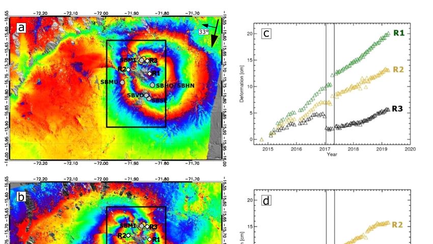
Remote Sens. 2020, 12, 1852                                                                        3 of 11

Hualca (Figure 1), similar to previous distributions [9]. AN analysis of the Sentinel-1, TerraSAR-X,
and COSMO-SkyMed missions from 2013–2018 found inflation northwest of Sabancaya as well as
creep and rupture on multiple faults [11]. Modelling of the inflation source showed that the location
(~7 km N of Sabancaya) and depth (~15 km) were consistent with the source inferred by [7].
     In this work, we present results relevant to the present volcanic unrest (October 2014 to March
2019). The DInSAR processing of an ascending and descending Sentinel 1 dataset and Global
Navigation Satellite System (GNSS) data analysis shows a radially symmetric inflation similar to the
one observed for 1992–1997 by [7]. The observed deformation field is compatible with a deep source,
12–15 km below the surface and 5 km north of Sabancaya, that has possibly been feeding the current
Sabancaya eruptions.

2. Deformation from DInSAR and GNSS

2.1. Synthetic Aperture Radar Data
      The SAR dataset consists of 84 ascending (Path 47, Frame 1125) and 79 descending orbit (Path 25,
Frames 614-646) scenes acquired by the Sentinel-1 Mission (European Space Agency, C-Band) between
October 2014 and March 2019. The acquisition mode is Interferometric Wide (IW). Sub-swath 2
of the ascending orbit and sub-swath 1 of the ascending orbit cover the whole area of interest
(Figure 1). They were processed using our own implementation of the DInSAR Small Baseline Subsets
(SBAS) time-series approach [12], which allows a proper spatial and temporal characterization of the
deformation patterns occurring within the studied area.
      We treated ascending and descending orbit scenes independently and computed deformation
time series and mean deformation velocity maps. We processed seven bursts of the sub-swath 2
for the ascending orbit and seven bursts of the sub-swath 1 for the descending orbit, and analyzed
254 ascending and 232 descending differential interferograms with maximum spatial and temporal
baselines of 163 m and 1374 days, respectively. Multilooking factors of 10 and 40 were applied in the
azimuth and range directions, respectively, giving a pixel of roughly 150 × 150 m. The topographic
fringes were removed via a 30 m Digital Elevation Model from NASA Shuttle Radar Topography
Mission (SRTM DEM) [13].
      We detected a significant contribution of topography-related fringes in most of the interferograms,
attributable to a stratified atmospheric phase component. This is particularly noticeable in the Cañon
del Colca region, a 1700 m-deep canyon to the North and West of the ASVC. To compensate for
the effect, which can cause a sinusoidal signal in the time series [14], we corrected each differential
interferogram using the Zenith Time Delay (ZTD) corrections provided by Newcastle University
through the Generic Atmospheric Correction Online Service (GACOS) [15] before a phase unwrapping
and time-series calculation.
      Because of the contribution from the atmosphere, the delay anomalies, the spatial averaging used
to down-sample the DInSAR data, and the structure of the noise in the DInSAR data estimate, it is
difficult to specify in a rigorous way the uncertainty in displacement measurements made with DInSAR.
On the basis of our own experience and consultations with colleagues who specialize in DInSAR,
we assigned an uncertainty to the DInSAR displacement measurements reported here of ±10 mm.

2.2. GNSS Data
     The GNSS volcanic deformation monitoring network, set up in ASVC by the Volcano Observatory
of the Instituto Geológico Minero y Metalúrgico (OVI-INGEMMET), has been collecting continuous
data since 2014. The network consists of five continuous GNSS stations that have been progressively
installed since October 2014. Three stations (SBVO, SBSE, and SBHN/SBHO) are within a 4 km
radius from Sabancaya, whereas the others (SBMI and SBMU) are 9 to 12 km away from the volcano.
SBHN and SBHO are the same station, but the name was changed in October 2016. Not all the stations
were operative during the time span covered by the DInSAR time-series (see Table 1).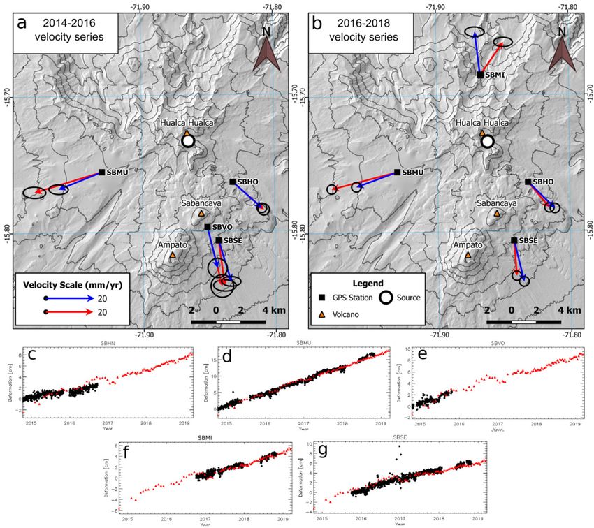
Remote Sens. 2020, 12, 1852                                                                       4 of 11

                       Table 1. GNSS stations with their corresponding data acquisition time.

                       GNSS Station                 Start Date                   End Date
                              SBVO              25 September 2014            25 October 2015
                               SBSE               3 October 2015             31 October 2018
                              SBMU              24 September 2014            31 October 2018
                              SBMI                5 October 2016             31 October 2018
                              SBHO                6 October 2016             31 October 2018
                              SBHN              26 September 2014           24 September 2016

     We used GAMIT/GLOBK v.10.70 [16] for processing the GNSS data. The carrier phase and other
observable data from satellites visible above a 10◦ elevation mask were sampled at 30 s intervals.
The daily position solutions were computed using precise ephemerides provided by the International
GNSS Service (IGS). The initial velocity solution was computed in the South America (SOAM)
reference frame defined by [17]. The position time series and preliminary velocities were adjusted
to 14 IGS stations located in the Stable South American (SSA) Plate, like POVE (Porto Velo, Brazil),
UNSA (Salta, Argentina), KOUR (Kourou, French Guiana), and MTV2 (Montevideo, Uruguay),
among others. The uncertainties of the GNSS velocities were derived by scaling the formal error by the
square root of the residual chi-square per the degrees of freedom of the solution (Table 2). We also
applied additional corrections, considering the monument instability (random walk), instrumental
error (white noise), and flicker noise [18].
     To eliminate the tectonic component of the deformation velocities observed at Sabancaya,
we employed the Euler pole and angular velocity of the Peruvian block. We first estimated the
tectonic deformation velocities from historical data from ten GPS stations active in southern Perú
between 2012 and 2014. Then, using these velocities, we calculated a Euler Pole [19] located in northern
Perú at 6.81◦ S and 72.52◦ W, with an angular velocity of 0.62◦ /My. Finally, the tectonic deformation
velocities for each GPS site of the Sabancaya monitoring network (located 1000 km away the Euler
Pole) are 11 ± 9 mm/yr east and 1 ± 1 mm/yr north.
     Given the stations’ availability (Table 1), the observed time span was split in two periods to
improve the outcomes from processing: October 2014 to October 2016, and October 2016 to October 2018.
The deformation velocity solutions for the first period include the SBMU, SBVO, SBSE, and SBHN
stations, whereas for the second period we have solutions from SBMU, SBSE, SBHO, and SBMI.

2.3. Modelling
     We inverted the deformation velocities for GNSS and DInSAR using the dMODELS package [20].
It implements analytical solutions for sources embedded in a homogeneous elastic half space.
This approach employs pressurized cavities of simple geometry to mimic/approximate the crustal
stress field produced by the actual source. None of these geometries reproduced an actual source.
We employed the inversion codes for spherical, spheroidal, and sill-like sources. dMODELS implements
a weighted least-squares algorithm combined with a random search grid to infer the minimum of the
penalty function, the chi-square per degree of freedom χ2v .
     We inverted the GNSS and DInSAR data independently. This allowed us to verify our modelling
results. For DInSAR, we searched for the parameters characterizing each model by jointly inverting the
ascending and descending orbits’ deformation velocities. This approach allowed us to better constrain
the source geometry, given that the deformation was projected in the Line-of-Sight (LOS, positive for
uplift in our images) direction. In order to reduce the computational cost, we down-sampled the original
data by a factor of 25 using a linear uniform subsampling method. In this case, given the low spatial
gradient of the displacement, we felt that it was not necessary to employ more complex algorithms,
such as gradient-based ones [21]. The inversion was performed using 17,640 measurements (pixels).
Remote Sens. 2020, 12, 1852 5 of 11
Remote Sens. 2020, 12, x FOR PEER REVIEW of
complex algorithms, such as gradient-based ones [21]. The inversion was performed using 17,640
3. Results measurements (pixels).
Figure 2 displays
3. Results
the results obtained by DInSAR processing. The mean deformation velocity in
the descending (Figure 2a) and ascending (Figure 2b) orbit reveals a deformation field centered on
Figure 2 displays the results obtained by DInSAR processing. The mean deformation velocity in
Hualca Hualca thevolcano
descendingbut affecting
(Figure 2a) and Ampato and Sabancaya
ascending (Figure volcanoes
2b) orbit reveals as well.
a deformation Its shape
field centered on is almost
circular, with Hualca
a diameter
Hualca of ~45 km,
volcano and itAmpato
but affecting appears andskewed
Sabancayain the opposite
volcanoes direction
as well. Its within Figure 2
shape is almost
because of thecircular, with a diameter of ~45 km, and it appears skewed in the opposite direction within Figure 2
SAR lateral view. The flight and LOS direction are indicated in the panels of Figure 2.
because of the SAR lateral view. The flight and LOS direction are indicated in the panels of Figure 2.
The LOS-projected maximum deformation
The LOS-projected is observed
maximum deformation in theinascending
is observed orbit
the ascending orbitand andreaches
reaches aa cumulative
displacement cumulative
of 20 cm.displacement of 20 cm.
Figure 2. TimeFigure
series extracted
2. Time at the positions
series extracted marked
at the positions marked R1, R2,
R1, R2, and
and R3 (white
R3 (white squares)squares) for deformation
for deformation
along the line of sight. Ascending and descending Sentinel-1 orbits (DInSAR) processing results for
along the line (a)
of sight. Ascending and descending Sentinel-1 orbits (DInSAR)
descending and (b) ascending orbits. SBMU, SBVO, SBSE, SBMI, and SBHO/SBHN are the
processing results for (a)
descending and (b) ascending
locations of the GNSSorbits.
stations. SBMU, SBVO,
(c) and (d) are the SBSE, SBMI,
deformation timeand SBHO/SBHN
series areand
of the descending the locations
ascending orbits,
of the GNSS stations. respectively,
(c) and (d) areextracted from R1, R2, and
the deformation R3 points.
time seriesTheofblack
thevertical lines mark
descending the ascending
and
time of the two 2017 earthquakes. The shape of the deformed area is almost circular, with a diameter
orbits, respectively, extracted
of ~45 km, from
and appears R1, R2,
skewed in theand R3 points.
opposite direction The
withinblack
Figurevertical
2 becauselines
of the mark the time of the
SAR lateral
view.
two 2017 earthquakes. The shape of the deformed area is almost circular, with a diameter of ~45 km,
and appears skewed in the opposite direction within Figure 2 because of the SAR lateral view.
In the descending orbit (Figure 2a,c), the significant shift observed in the first months of 2017 is
related to two earthquakes of magnitude Mw = 3.8 and Mw = 3.4 which occurred on January 15 and
In the descending orbit
30 April 2017, (Figure
respectively. 2a,c),
The the significant
time series at R3, the pixelshift observed
nearest in theshows
to the epicenters, first an
months
offset of 2017 is
related to twoofearthquakes
almost 2.5 cm of
ofLOS
magnitude Mwto=the
decrease linked 3.8first
and Mw = 3.4
earthquake. Thewhich
other two pixels (R1 on
occurred andJanuary
R2), 15 and
30 April 2017, respectively. The time series at R3, the pixel nearest to the epicenters, shows an offset
of almost 2.5 cm of LOS decrease linked to the first earthquake. The other two pixels (R1 and R2),
located at the centers of the LOS-projected regional volcanic deformation patterns, show shifts linked
to the second earthquake. In the latter case, the fringes suggest a LOS increase around 1 cm.
The series taken from the ascending orbit do not present such a clear interpretation due to the low
data availability (no acquisition) between 2014 and mid-2016, resulting in a low temporal resolution.
The earthquake signals are not as strong as in the descending orbit, probably because of the relative
orientation between the deformation and the sensor flight direction. However, minor shifts coincident
with the 30 April 2017 earthquake are observed.
The earthquakes’ signals are superimposed on the time series to the linear trend of the regional
volcanic deformation. The regional volcanic deformation would be almost linear during the analyzed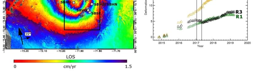
Remote Sens. 2020, 12, 1852                                                                            6 of 11

time span and is perturbed by the two rupture events shown in Figure 2c,d. The deformation mean
velocity before and after the earthquakes is very similar, about 35 to 50 mm/yr. The pixels near
the epicenters—R3 in Figure 2c—also show a year-long post-seismic relaxation effect followed by
a progressive velocity increase.

      Table 2. Summary of the calculated GNSS velocities per pre-eruptive and eruptive stage (before and
      after the beginning of the eruption of Sabancaya). The values are in millimeters per year (mm/yr).

                                       SBVO        SBMU       SBHN/SBHO SBSE             SBMI
                              E        5±2         −24 ± 2      11 ± 1        2±2
               10/14–10/16    N       −21 ± 2      −7 ± 1       −10 ± 1      −16 ± 1
                              U        25 ± 6       33 ± 4      34 ± 3       27 ± 7
                                   Sabancaya Eruption (6 November 2016)
                              E                    −28 ± 1       9±1          1±1        10 ± 2
               10/16–10/18    N                    −7 ± 1       −11 ± 1      −15 ± 1     14 ± 1
                              U                     26 ± 6      29 ± 3       17 ± 5      26 ± 6

     Figure 3 and Table 2 display the mean deformation velocity (red vectors in Figure 3) computed from
the GNSS data. The horizontal components, excluding station SBMI, show a radial deformation centered
near Hualca Hualca between October 2016 and October 2018, affecting the whole Ampato-Sabancaya
volcanic complex. SBMI is located between the epicenters of the two earthquakes in 2017, so this
velocity vector is affected by co- and post-seismic displacement. The vertical components are positive,
varying between 1.7 and 3.4 cm/year. These results are consistent with the deformation measured by
DInSAR (Figure 3c–g).

Modelling
      Table 3 shows the inversion results using both the GNSS and the DInSAR data. To avoid the local
effect of the earthquakes (e.g., post-seismic relaxation), we divided the deformation from the DInSAR
time series into two periods. The first period is from October 2014 to December 2016, the second from
January 2018 to March 2019. The GNSS data have also been split into two time spans linked to station
availability (Table 2).
      The results for both the time spans are detailed in Table 3. The independent inversion of the GNSS
and DInSAR deformation data infers a deep source close to Hualca Hualca as the most probable result
in all the modelled geometries.
      The sill-like geometry, more appropriate for local deformation patterns produced by shallow
sources, yielded parameters geologically implausible (e.g., extremely large radius or near surface
depths), so we discarded it.
      Of the remaining geometries, the spherical source model better fits both periods with GNSS and
DInSAR data. Since the misfit is very similar, we prefer the simpler spherical source (four parameters)
to the spheroidal source (seven parameters). The locations from the four best-fit inversions are within
a 2 km radius area beneath Hualca Hualca. The dimensionless pressure change is well within the
validity range of the linear elasticity assumption of the analytical model (0–0.1). The best fit models
employing a spheroidal geometry infer a deeper source (~16 km) and produce a greater geographic
dispersion between the best-fit results of the GNSS and DInSAR data.
      The best fit for the independent inversion of GNSS and DInSAR data for the first period has
a 12–14 km deep and 1.5 km-radius spherical source located beneath Hualca Hualca. Its volume change
rate is between 26 × 106 m3 /yr and 43 × 106 m3 /yr, the dimensionless pressure change between 0.002
and 0.004, and the χ2 v between 1.0 and 2.8.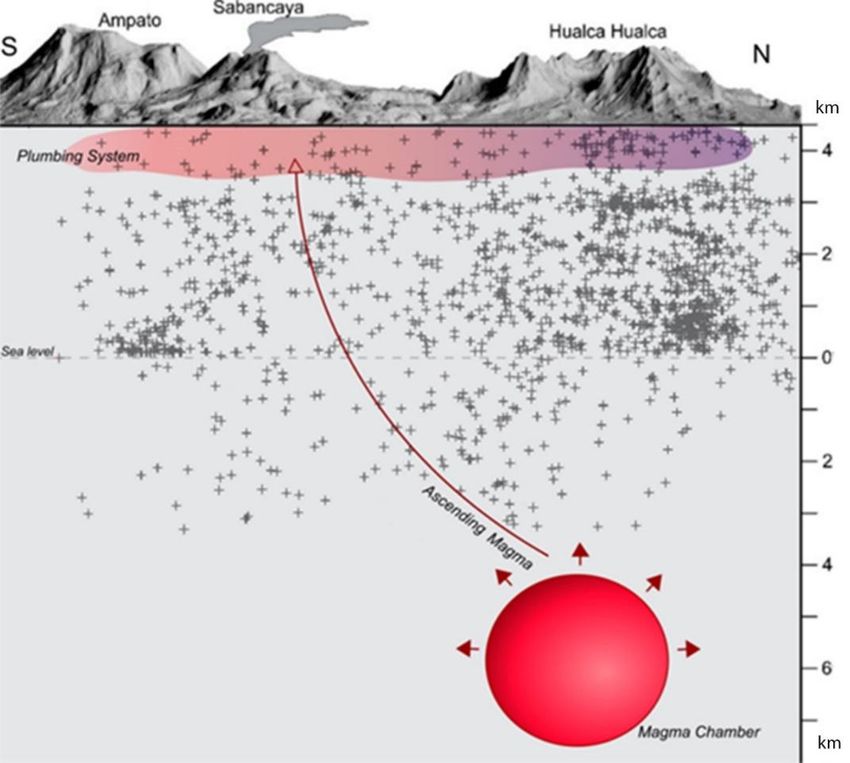
Remote Sens. 2020, 12, 1852 7 of 11
Table 3. Parameters of the best-fit sources for each period for both data sets for all geometries. Depth is
relative to Sabancaya’s vent.
Lat Long Depth Radius δV
Period Geometry Data χ2 v ◦ ◦ δP
km km ×106 m3
10/2014–12/2016 Sphere DInSAR 1.0 −15.7225 ± 0.0027 −71.8727◦ 15 ± 1 1.5 0.004 ±0.001 43 ± 5
10/2014–12/2016 Spheroid DInSAR 6.6 −15.7407 −71.9345◦ 15.1 1.5 0.009 32
10/2014–12/2016 Sill DInSAR 6.6 −15.7438 −71.8468◦ 15.6 10.9 0.0001 26
09/2014–11/2016 Sphere GNSS 2.8 −15.7335 ± 0.0027 −71.8648◦ 12 ± 1 1.5 0.002 ±0.001 26 ± 4
09/2014–11/2016 Spheroid GNSS 1.0 −15.7391 −71.8624◦ 9.3 1.5 0.481 20
11/2016–11/2018 Sphere GNSS 25.5 −15.7340 ± 0.0027 −71.8618◦ 11 ± 1 1.5 0.002 ±0.001 22 ± 4
11/2016–11/2018 Sill GNSS 17.9 −15.7306 −71.8680◦ 1.2 1.5 0.052 18
01/2018–4/2019 Sphere DInSAR 1.7 −15.7159 ± 0.0027 −71.8563◦ 15.3 ± 0.9 1.5 0.005 ±0.001 51 ± 4
Remote Sens. 2020, 12, x FOR PEER REVIEW of
The independent inversion for the second GNSS and DInSAR deformation velocity series yields
The best
similar results (Table fit forspherical
3). The the independent
sourceinversion of GNSS
is located at and DInSAR
nearly thedata
samefor position
the first period
andhas a
depth (12–15 km)
12–14 km deep and 1.5 km-radius spherical2 source located beneath Hualca Hualca. Its volume change
for both data rate
sets. Despite a much higher χ for the GNSS inversion, the volume change rate is of
is between 26 × 106 m3/yr and 43 × 106 vm3/yr, the dimensionless pressure change between 0.002
the same order andof0.004,
magnitude
and the χ2v (see
betweenTable 3).2.8.
1.0 and We calculated the errors for the best-fit parameters using
the Monte Carlo The independenttechnique
simulation inversion for [22].
the second
WeGNSS
added and white
DInSARnoise
deformation
to thevelocity series yields
original data set and then
similar results (Table 3). The spherical source is located at nearly the same position and depth (12–15
inverted it forkm)
theforbest
bothfit solution.
data Wea much
sets. Despite repeated
higherthis
χ2v forprocess
the GNSS100 times.
inversion, theThe
volume errors
changepresented
rate is in Table 3
reflect the distribution
of the same of ordertheof solutions
magnitude (seefound.
Table 3). We calculated the errors for the best-fit parameters
using the Monte Carlo simulation technique [22]. We added white noise to the original data set and
Figure 3 presents the horizontal velocity vectors produced by the GNSS best-fit spherical sources
then inverted it for the best fit solution. We repeated this process 100 times. The errors presented in
(blue vectors).Table
Note howthethe
3 reflect SBMI station
distribution shows
of the solutions a noticeable difference between the observed and
found.
modelled velocity. Figure
This 3 presents
station thewas
horizontal velocity
affected byvectors produced
the 2017 by the GNSS
seismic events,best-fit
sospherical
it recordedsourcesthe combined
(blue vectors). Note how the SBMI station shows a noticeable difference between the observed and
effect of the underlying regional pattern and the local earthquakes’ deformation field. Using data
modelled velocity. This station was affected by the 2017 seismic events, so it recorded the combined
provided by the SBMI
effect of the station
underlying results
regionalinpattern
a higher χ2local
and the v value (~25) and
earthquakes’ a smaller
deformation field. fit.
Using The
datamodelled and
observed dataprovided
present byathe SBMI station results
significantly betterin afit
higher χ2v value
at the other(~25) and a smaller fit. The modelled and
stations.
observed data present a significantly better fit at the other stations.
Figure 3. Horizontal velocity vectors produced by the best-fit spherical source (blue) and GNSS data
Figure 3. Horizontal
(red) for (a)velocity vectors
the 2014–2016 produced
velocity by
series and (b) thethe best-fit
2016–2018 spherical
velocity source
series. Note (blue)
how the and GNSS data
data and
(red) for (a) the 2014–2016 velocity series and (b) the 2016–2018 velocity series. Note how the data and
modelled vectors of the SBMI station differ because of a nearby seismic event. (c–g) GNSS
deformation series, projected into the ascending Line-of-Sight (LOS), compared to the ascending
modelled vectors of the SBMI station differ because of a nearby seismic event. (c–g) GNSS deformation
DInSAR series.
series, projected into the ascending Line-of-Sight (LOS), compared to the ascending DInSAR series.
The pattern and residuals obtained by modelling the DInSAR data are presented in Figure 4.
After subtracting the modeled component, the possible seismic effects are observed in the residual
The pattern and residuals obtained by modelling the DInSAR data are presented in Figure 4.
from both the analyzed periods and are especially noteworthy in 2014–2017. The main seismic
After subtracting the modeled
deformation component,
pattern located the possible
NE of Sabancaya seismic
volcano could effects are
be associated withobserved ineffect
a post-seismic the residual from
related to the Mw = 5.9 earthquake on 17 July 2013 [9].Remote Sens. 2020, 12, 1852 8 of 11
both the analyzed periods and are especially noteworthy in 2014–2017. The main seismic deformation
pattern located NE
Remote Sens. of12,Sabancaya
2020, volcano could be associated with a post-seismic effect related
x FOR PEER REVIEW of to the
Mw = 5.9 earthquake on 17 July 2013 [9].
Figure 4.Figure 4. Spherical
Spherical source source
modelmodel results
results forfor theDInSAR
the DInSAR data
data(a)
(a)2014–2016 ascending
2014–2016 and descending
ascending and descending
series and (b) 2018–2019 ascending and descending series. First column is the full resolution DInSAR
series and (b) 2018–2019 ascending and descending series. First column is the full resolution
data, the second column is the inverse modelling result, and the third column is the residual between
DInSAR
data, thethe
second column is the inverse modelling result, and the third column is the residual
data and model. Note how the seismic deformation, still ongoing, is evident in the residuals of between
the data both
andseries.
model. Note how the seismic deformation, still ongoing, is evident in the residuals of
both series.
4. Discussion
The analysis and interpretation of the DInSAR and GNSS deformation data allow us to better
understand the Sabancaya volcanic system. In particular, our analysis shows that ground deformation
affects the three volcanic edifices of the Ampato-Sabancaya volcanic complex (Figures 2 and 3).
Deformation patterns and best-fit sources (Figure 5) are centered more than 5 km away from the
eruptive vent, close to Hualca Hualca. This lateral magmatic deformation zone is a common feature
of volcanic unrest. According to a survey by [23], 24% of monitored volcanoes have had similar
deformation signals.Remote Sens. 2020, 12, 1852 9 of 11
A linear deformation trend is observed throughout the entire time span. This trend is caused by
magmatic deformation disturbed by local seismicity (Figure 2). To minimize the influence of seismic
deformation on our models, we split the DInSAR and GNSS velocity series into two periods—before and
after the 2017 seismic events (Figure 2). The offset and long-term trends observed in the time series
after the 2017 seismic events (Figure 2) are the effect of a rapid co-seismic deformation followed by
a possible slower post-seismic relaxation.
The deformation source inferred by the independent inversion of the DInSAR and GNSS
deformation velocities shows a deep source (12–15 km below the surface) beneath Hualca Hualca with
a volume change rate of 26–43 × 106 m3 /yr, in agreement with the results obtained by [24] for the same
period. The residuals in the DInSAR data are related to seismic deformation and provide a clear view
of the faults’ movement. The model fits very well also with the deformation velocity vectors from the
GNSS (Figure 3a,b). The station SMBI is affected by the earthquakes and has a combined signal from
the local volcanic source and the regional seismic deformation.
The results obtained by the inversion of the GNSS data validate the DInSAR best-fit model,
with both having similar locations, depths, and volume change rates. Furthermore, the similar results
for both the deformation velocity series reinforce the linear trend hypothesis for the whole period
(Figure 3c–g).
The best-fit source, located between 12 and 15 km beneath Hualca Hualca, reproduces the stress
field and volume change of a magma reservoir that might have fed Sabancaya’s eruptions since
the mid-1990s.
Remote Sens. 2020, 12, x FOR PEER REVIEW of
Figure 5. Conceptual model of the Sabancaya magmatic system. The 1.5 km radius sphere reproduces
Figure 5. Conceptual model of the Sabancaya magmatic system. The 1.5 km radius sphere reproduces
the stress field and volume change of a magma chamber at 12–15 km depth beneath Hualca Hualca.
the stress field
Red linesand volumeascending
are possible change of a magma
paths chamber
of magmatic atthe
fluids to 12–15 km depth
Sabancaya beneath
conduit and theHualca
extensiveHualca.
Red linesplumbing
are possible ascending
system. paths
Black crosses of magmatic
represent fluids
earthquakes to theduring
occurred Sabancaya conduit
the analyzed and
time the extensive
span.
plumbing system. Black crosses represent earthquakes occurred during the analyzed time span.
The deep intrusion of magma into an existing reservoir can cause the migration of magmatic
The deepinto
fluids the ASVCofplumbing
intrusion magmasystem andexisting
into an a changereservoir
in the local can
heat cause
flow [10].
theThe volume/pressure
migration of magmatic
change started a period of volcanic unrest with inflation accompanied by seismicity. The epicenters
fluids into the ASVC plumbing system and a change in the local heat flow [10]. The volume/pressure
of the earthquakes produced by fluid movements along permeable pathways and fault structures
change started a period
concentrate of Hualca
north of volcanic unrest
Hualca. with and
Magma inflation accompanied
hydrothermal by seismicity.
fluids, driven The epicenters
by convection, can
of the earthquakes produced by fluid
reach Sabancaya’s conduit (Figure 5).movements along permeable pathways and fault structures
Our results confirm the existence of a previous inflation episode in the 1990′s [7], with ground
deformation centered on Hualca Hualca. In our opinion, Sabancaya is fed by a laterally extensive
magmatic plumbing system (Figure 5) which allows fluids to move along a highly fractured (Figure
1) and pressured crust from the “offset” deep magma chamber to their emission point.
5. ConclusionsRemote Sens. 2020, 12, 1852 10 of 11
concentrate north of Hualca Hualca. Magma and hydrothermal fluids, driven by convection, can reach
Sabancaya’s conduit (Figure 5).
Our results confirm the existence of a previous inflation episode in the 19900 s [7], with ground
deformation centered on Hualca Hualca. In our opinion, Sabancaya is fed by a laterally extensive
magmatic plumbing system (Figure 5) which allows fluids to move along a highly fractured (Figure 1)
and pressured crust from the “offset” deep magma chamber to their emission point.
5. Conclusions
Continuous GNSS measurements and DInSAR observation from the ascending and descending
Sentinel-1 tracks show a large inflation pattern (~45 km diameter) affecting the ASVC. The beginning
date of the inflation is uncertain. The analyzed deformation velocity series have an almost linear
trend for the whole period, interrupted by local seismic events. To minimize the local effect of the
earthquakes on modelling, we divide both the DInSAR and GNSS data into two series: one before
the 2017 earthquakes (October 2014 to December 2016) and one after the post-seismic relaxation
(January 2018 to March 2019). For both datasets, the best-fit source is a deep intrusion (12 to 15 km
below the surface) beneath Hualca Hualca. This is the same source inferred by [7] for the unrest
experienced by Sabancaya in the mid-1990s. The regional inflation pattern centered on Hualca Hualca,
the “offset” magma chamber, and the concentration of seismic activity north of ASVC suggest that
a laterally extensive magmatic plumbing system may be responsible for this deformation scenario.
Author Contributions: Data processing, modelling, and writing—original draft preparation, G.B. and
L.F.C.; resources and project supervision, R.M.C.; data curation and advising, P.A.E. and L.D.E.; software,
conceptualization, writing—review and editing, M.B. All authors have read and agreed to the published version
of the manuscript.
Funding: L. Cruz was funded by the Universidad Nacional de San Agustín de Arequipa and the UNSA-INVESTIGA
program under contract No. TP-013-2018-UNSA. Funding for this work came from USAID via the Volcano
Disaster Assistance Program and from the U.S. Geological Survey (USGS) Volcano Hazards Program.
Acknowledgments: We thank Chris Harpel (USGS), Chuck Wicks (USGS), and four anonymous reviewers for
improving this work with their constructive comments. Any use of trade, firm, or product names is for descriptive
purposes only and does not imply endorsement by the U.S. Government.
Conflicts of Interest: The authors declare no conflict of interest.
References and Note
1. Rivera, M.; Mariño, J.; Samaniego, P.; Delgado, R.; Manrique, N. Geología y evaluación de peligros del complejo
volcánico Ampato-Sabancaya (Arequipa). INGEMMET Boletín Serie C Geodinámica e Ingeniería Geológica 2015,
61, 122.
2. Samaniego, P.; Rivera, M.; Mariño, J.; Guillou, H.; Liorzou, C.; Zerathe, S.; Delgado, R.; Valderrama, P.;
Scao, V. The eruptive chronology of the Ampato–Sabancaya volcanic complex (Southern Peru). J. Volcanol.
Geotherm. Res. 2016, 323, 110–128. [CrossRef]
3. Ciesielczuk, J.; Żaba, J.; Bzowska, G.; Gaidzik, K.; Głogowska, M. Sulphate efflorescences at the geyser near
Pinchollo, southern Peru. J. South Am. Earth Sci. 2013, 42, 186–193. [CrossRef]
4. Siebert, L.; Simkin, T.; Kimberly, P. Volcanoes of the World, 3rd ed.; University of California Press:
London, UK, 2010.
5. Thouret, J.; Guillande, R.; Huamán, D.; Gourgaud, A.; Salas, G.; Chorowicz, J. L’activité actuelle du Nevado
Sabancaya (Sud Pérou): Reconnaissance géologique et satellitaire, évaluation et cartographie des menaces
volcaniques. Bulletin de la Société Géologique de France 1994, 165, 49–63.
6. Huamán, D. Métodos y Aplicaciones de las Imágenes de Satélite en la Cartografía Geológica: El caso del
Seguimiento y Evolución de la Amenaza Volcánica del Sabancaya (región del Colca, Arequipa, Perú). Tesis de
Ingeniero Geólogo, Universidad Nacional de San Agustín, Arequipa, Peru, 1995.
7. Pritchard, M.E.; Simons, M. An InSAR-based survey of volcanic deformation in the central Andes.
Geochem. Geophys. Geosystems 2004, 5, 2. [CrossRef]Remote Sens. 2020, 12, 1852 11 of 11
8. Ramos, D.; Masías, P.; Apaza, F.; Lazarte, I.; Taipe, E.; Miranda, R.; Ortega, M.; Anccasi, R.; Ccallata, B.;
Calderón, J.; et al. Los inicios de la actividad eruptiva 2016 del volcán Sabancaya. INGEMMET Informe
Técnico n◦ A6735, 2016.
9. Jay, J.; Delgado, F.; Torres, J.; Pritchard, M.; Macedo, O.; Aguilar, V. Deformation and seismicity near
Sabancaya volcano, southern Peru, from 2002 to 2015. Geophys. Res. Lett. 2015, 42, 2780–2788. [CrossRef]
10. Reath, K.; Pritchard, M.E.; Moruzzi, S.; Alcott, A.; Coppola, D.; Pieri, D. The AVTOD (ASTER Volcanic
Thermal Output Database) Latin America archive. J. Volcanol. Geotherm. Res. 2019, 376, 62–74. [CrossRef]
11. MacQueen, P.; Delgado, F.; Reath, K.; Pritchard, M.; Lundgren, P.; Milillo, P.; Macedo, O.; Aguilar, V.; Zerpa, I.;
Machacca, R.; et al. Volcano-tectonic interactions at Sabancaya volcano, Peru (2013–2018): Eruptions,
magmatic inflation, moderate earthquakes, and aseismic slip. Am. Geophys. Union Fall Meet V23C-03 2018.
12. Berardino, P.; Fornaro, G.; Lanari, R.; Sansosti, E. A new algorithm for surface deformation monitoring based
on small baseline differential SAR interferograms. IEEE TGARS 2002, 40, 2375–2383. [CrossRef]
13. Farr, T.G.; Rosen, P.A.; Caro, E.; Crippen, R.; Duren, R.; Hensley, S.; Kobrick, M.; Paller, M.; Rodriguez, E.;
Roth, L.; et al. The Shuttle Radar Topography Mission. Rev. Geophys. 2007, 45, RG2004. [CrossRef]
14. Samsonov, S.V.; Trishchenko, A.P.; Tiampo, K.; González, P.J.; Zhang, Y.; Fernández, J. Removal of systematic
seasonal atmospheric signal from interferometric synthetic aperture radar ground deformation time series.
Geophys. Res. Lett. 2014, 41, 6123–6130. [CrossRef]
15. Yu, C.; Li, Z.; Penna, N.T.; Crippa, P. Generic Atmospheric Correction Model for Interferometric Synthetic
Aperture Radar Observations. J. Geophys. Res. Solid Earth 2018, 123, 9202–9222. [CrossRef]
16. Herring, T.; King, R.W.; McCluskey, S.M. Introduction to GAMIT/GLOBK Release 10.7. In Massachusetts
Institute of Technology Technical Report; Massachusetts Institute of Technology: Cambridge, MA, USA, 2018.
Available online: http://geoweb.mit.edu/gg/ (accessed on 5 May 2020).
17. Altamimi, Z.; Métivier, L.; Collilieux, X. ITRF2008 plate motion model. J. Geophys. Res. Solid Earth 2012, 117.
[CrossRef]
18. Williams, S.D.; Bock, Y.; Fang, P.; Jamason, P.; Nikolaidis, R.M.; Prawirodirdjo, L.; Miller, M.; Johnson, D.J.
Error analysis of continuous GPS position time series. J. Geophys. Res. Solid Earth 2004, 109. [CrossRef]
19. Forsythe, R.D.; Davidson, J.; Mpodozis, C.; Jesinkey, C. Lower Paleozoic relative motion of the Arequipa
Block and Gondwana; paleomagnetic evidence from Sierra de Almeida of northern Chile. Tectonics 1993, 12,
219–236. [CrossRef]
20. Battaglia, M.; Cervelli, P.F.; Murray, J.R. dMODELS: A MATLAB software package for modelling crustal
deformation near active faults and volcanic centers. J. Volcanol. Geotherm. Res. 2013, 254, 1–4. [CrossRef]
21. Decriem, J.; Árnadóttir, T.; Hooper, A.; Geirsson, H.; Sigmundsson, F.; Keiding, M. The 2008 May 29
earthquake doublet in SW Iceland. Geophys. J. Int. 2010, 181, 1128–1146. [CrossRef]
22. Wright, T.; Fielding, E.; Parsons, B. Triggered slip: Observations of the 17 August 1999 Izmit (Turkey)
earthquake using radar interferometry. Geophys. Res. Lett. 2001, 28, 1079–1082. [CrossRef]
23. Ebmeier, S.K.; Andrews, B.J.; Araya, M.C.; Arnold, D.W.D.; Biggs, J.; Cooper, C.; Cottrell, E.; Furtney, M.;
Hickey, J.; Jay, J.; et al. Synthesis of global satellite observations of magmatic and volcanic deformation:
Implications for volcano monitoring & the lateral extent of magmatic domains. J. Appl. Volcanol. 2018, 7, 2.
[CrossRef]
24. MacQueen, P.; Delgado, F.; Reath, K.; Pritchard, M.E.; Bagnardi, M.; Milillo, P.; Lundgren, P.; Macedo, O.;
Aguilar, V.; Ortega, M.; et al. Volcano-tectonic interactions at Sabancaya volcano, Peru: Eruptions,
magmatic inflation, moderate earthquakes, and fault creep. J. Geophys. Res. Solid Earth 2020. [CrossRef]
© 2020 by the authors. Licensee MDPI, Basel, Switzerland. This article is an open access
article distributed under the terms and conditions of the Creative Commons Attribution
(CC BY) license (http://creativecommons.org/licenses/by/4.0/).You can also read