G-MIND: An End-to-End Multimodal Imaging-Genetics Framework for Biomarker Identification and Disease Classification
←
→
Page content transcription
If your browser does not render page correctly, please read the page content below
G-MIND: An End-to-End Multimodal Imaging-Genetics
                                                  Framework for Biomarker Identification and Disease
                                                                   Classification
                                             Sayan Ghosal1 , Qiang Chen2 , Giulio Pergola2,4 , Aaron L. Goldman2 , William Ulrich2 , Karen
                                             F. Berman3 , Giuseppe Blasi4,5 , Leonardo Fazio4 , Antonio Rampino4 , Alessandro Bertolino4 ,
                                                     Daniel R. Weinberger2 , Venkata S. Mattay2 , and Archana Venkataraman1
                                                 1
                                                  Department of Electrical and Computer Engineering, Johns Hopkins University, USA
arXiv:2101.11656v1 [q-bio.QM] 27 Jan 2021

                                                                      2
                                                                        Lieber Institute for Brain Development, USA
                                                          3
                                                            Clinical and Translational Neuroscience Branch, NIMH, NIH, USA
                                              4
                                                Department of Basic Medical Sciences, Neuroscience and Sense Organs, University of Bari
                                                                                      Aldo Moro, Italy
                                                        5
                                                          Azienda Ospedaliero-Universitaria Consorziale Policlinico, Bari, Italy

                                                                                              ABSTRACT
                                            We propose a novel deep neural network architecture to integrate imaging and genetics data, as guided by
                                            diagnosis, that provides interpretable biomarkers. Our model consists of an encoder, a decoder and a classifier.
                                            The encoder learns a non-linear subspace shared between the input data modalities. The classifier and the
                                            decoder act as regularizers to ensure that the low-dimensional encoding captures predictive differences between
                                            patients and controls. We use a learnable dropout layer to extract interpretable biomarkers from the data, and
                                            our unique training strategy can easily accommodate missing data modalities across subjects. We have evaluated
                                            our model on a population study of schizophrenia that includes two functional MRI (fMRI) paradigms and Single
                                            Nucleotide Polymorphism (SNP) data. Using 10-fold cross validation, we demonstrate that our model achieves
                                            better classification accuracy than baseline methods, and that this performance generalizes to a second dataset
                                            collected at a different site. In an exploratory analysis we further show that the biomarkers identified by our
                                            model are closely associated with the well-documented deficits in schizophrenia.
                                            Keywords: Deep Neural Networks, Learnable Dropout, Imaging-Genetics, Schizophrenia

                                                                                        1. INTRODUCTION
                                            Neuropsychiatric disorders, such as autism and schizophrenia, are typically characterized by cognitive and behav-
                                            ioral deficits.1 At the same time, these diseases also show high genetic heritability,2 which suggests an important
                                            link between genotypic variations and the observed phenotypic traits.3 Understanding this relationship might
                                            lead to targeted biomarkers and eventually better therapeutics. Non-invasive techniques like functional MRI
                                            (fMRI) and Single Neucleotide Polymorphism (SNP) are commonly used data modalities to capture the brain
                                            activity and genetic variations, respectively. However, integrating them in a single framework is hard due to their
                                            inherent complexity, high data dimensionality, and our limited knowledge about the underlying relationships.
                                                Imaging-genetics has become an increasingly popular field of study to link these modalities. Data driven
                                            methods can be grouped into three categories. The first category uses multivariate regularized regression to model
                                            the effect of genetic variations on the brain activity.4, 5 These methods rely on sparsity to identify an interpretable
                                            set of biomarkers; however, they do not incorporate clinical diagnosis, meaning that the biomarkers may not align
                                            with predictive group differences. The second category uses correlation analysis to identify associations between
                                            genetic variations and quantitative traits.6–8 However, the representations are rarely guided by the clinical
                                            factors, and it is not clear how they can be extended to accommodate more than two data modalities. Finally,
                                            the recent works of 9, 10 use probabilistic modelling and dictionary learning, respectively, to integrate imaging,
                                            genetics, and diagnosis. The generative nature of these methods makes it harder to integrate additional data
                                            modalities. However, the field is moving towards multimodal imaging acquisitions to capture different snapshots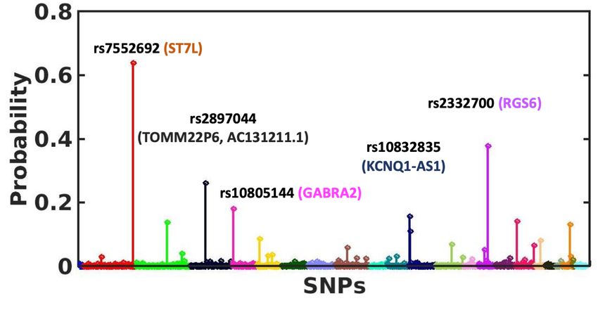
Figure 1: G-MIND architecture. The inputs {i1 , i2 } and {g} corresponds to the two imaging modalities and
genetic data, respectively. Ei (·) and Di (·) captures the encoding and decoding operations, and Y(·) captures the
classification operation. zi is the learnable dropout mask, and `n is the low dimensional latent space.

of the brain all of which may have link to the genotype. Another limitation is that none of the above methods can
handle the problem of missing data. With the growing emphasis on big datasets comes the challenge of missing
data modalities. Traditionally, missing data has been managed by removing subjects from the analysis,11 which
does not make use of all the information. In this paper we introduce a novel model and training strategy that
accommodates these missing modalities to maximize the size and utility of the dataset.
    The above limitations have motivated our use of deep learning, and specifically, the autoencoder architecture.
First, the autoencoder provides a natural way to integrate new data modalities12 simply by adding new encoder-
decoder branches. Mathematically, a new branch will introduce another term to the loss function but does not
alter the optimization procedure (e.g., backpropagating gradients).13 Second, missing data can easily be handled
by freezing the affected part of the network14 and updating the remaining weights. This simplicity is in stark
contrast to the classical methods, where the entire model and optimization procedure must be changed for each
new modality and missing data configuration. Third, the latent encoding provides a data-driven feature space
that can be used for patient/control classification. Again, this is in contrast to classical approaches, which are
highly dependent on hand-crafted feature. Finally, the classifier part of our model guides the autoencoder to
extract clinically interpretable features that are representative of the disease.
    In this paper we introduce the Genetic and Multimodal Imaging data using Neural-network Designs (G-
MIND) framework to identify predictive biomarkers from neuroimaging and genetics data for disease diagnosis.
We use a coupled autoencoder and classifier to learn a shared latent space among all the input modalities that
is representative of the population differences between patients and controls. We also incorporate a learnable
dropout layer15 by which the model selects a random subset of input features to pass to the encoder. The feature
importances are captured in the probability of dropout, which is learned via backpropagation. We evaluate G-
MIND on a study of schizophrenia that includes two task fMRI paradigms and SNP data. Our method achieves
better classification performance than standard baselines and also identifies clinically relevant biomarkers. We
further applied G-MIND to a cross-site dataset without any fine tuning to show the transferability of our model.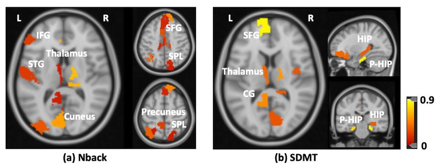
2. THE MULTI-MODAL ENCODER-DECODER FRAMEWORK
Fig. 1 illustrates our full model. The inputs in1 and in2 denotes the input imaging modalities for subject n. In
our case in1 and in2 are activation maps from two different fMRI paradigms. The input gn represents the SNP
genotype, and y n is a binary class label (patient or control). Let N1 , N2 , and Ng denote the number of subjects
from whom we have the corresponding imaging or genetic modality. Let R be the total number of ROIs in
brain, and G be the total number of SNPs. The imaging data has the dimensionality in1 , in2 ∈ RR×1 , and the
genetic data has the dimensionality gn ∈ RG×1 . We jointly model the imaging and genetic modalities using a
auto-encoder framework. The first layer of the encoder incorporates a learnable dropout parameterized by pm
for each modality m. We use the resulting low dimensional representation `n for subject classification.

2.1 Feature Importance using Learnable Dropout
The standard Bernoulli dropout independently drops nodes using a fixed probability. The Bayesian interpretation
of dropout has a close resemblance with Bayesian feature selection,16 however, the user must fix the dropout
probability a priori. Here we wish to learn these vales, so we reparameterize the Bernoulli dropout mask with a
Gumbell-Softmax17 distribution. This continuous relaxation of Bernoulli random variable enables us to update
the dropout probabilities while training the network. During each forward pass through the network we sample
random variables zni1 , zni2 ∈ RR×1 , and zg ∈ RG×1 for imaging and genetic data, respectively, from a Gumbell-
Softmax distribution and use it as a dropout mask for patient n:
                                         log(pi1 ) − log(1 − pi1 ) + log(uni1 ) − log(1 − uni1 )

                              zni1 = σ                                                                      (1)
                                                                   t

where uni1 is a random vector sampled from U nif orm(0, 1), the parameter t (temperature) controls the extent of
relaxation from the Bernoulli distribution and pm captures the probabilities with which the features of modality m
are selected. As seen in Eq. (1) when the probability pmk is close to 1 that feature will be selected most of the
time, as compared to a feature whose probability is close to 0. We further incorporate a sparsity penalty over
the probabilities pmk via the KL divergence KL (Ber(q)||Ber(pmk )) where q is a hyperparameter fixed to 0.001.
Effectively, this term encourages pmk towards zero for all features.

2.2 Multimodal Latent Encoding
The encoder learns a nonlinear latent space that is shared between all the data modalities. As shown in Fig. 1 we
encode the data following the dropout using a cascade of fully connected layers followed by a PRelu activation.18
Unlike standard autoencoder based networks we couple the low dimensional representations of each data modality
to leverage the common structures shared between them. The latent embedding `n is computed as
                                          1
                                  `n =      E1 (in1 , zni1 ) + E2 (in2 , zni2 ) + Eg (gn , zng )

                                                                                                                (2)
                                         Mn
Here Ei (·) represents the encoding operation for modality m, and Mn is the number of modalities present for
subject n. As seen in Eq. (2), our latent representation is the sum of the individual projections, scaled by the
amount of available data Mn . This fusion strategy encourages the latent encoding for an individual patient to
have a consistent scale, even when constructed using a subset of the modalities.

2.3 Data Reconstruction
The decoder reconstructs the data from the latent representation to ensure that the encoder is preserving sufficient
information about the inputs. We use fully connected layers along with PRelu, dropouts, and batchnorm for
decoding. Mathematically, the autoencoder loss is the l2 norm between the input and reconstruction:
                         n1                         N2                             Ng
                         X                          X                              X
                              ||iN        n 2
                                 1 − D1 (` )||2 +         ||in2 − D2 (`n )||22 +         ||gn − D3 (`n )||22
                        n=1                         n=1                            n=1

where Dm (·) is the decoding operation for modality m.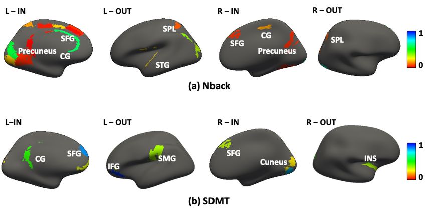
Modalities
                                                                                                       Institution
                                                                                                                       NBack        SDMT       SNP
                                                                                                          LIBD           160           110     210
                                                                                                          BARI            97                   97

Figure 2: Information flow during the forward pass                                                  Table 1: The number of subjects present
(green) and backward pass (red) when in1 is absent.                                                 for each modality from the two institutions.
                                                                                                    Note that the SDMT task was not acquired
                                                                                                    for BARI

2.4 Disease Classification
The final piece of our network is a classifier for disease prediction, which will encourage the dropout mask and
latent embeddings to select discriminative
                                   PN       features from the data. We employ fully connected layers, and a cross
entropy loss for classification: − n=1 (y n log(ŷ n ) + (1 − y n ) log(1 − ŷ n )), where y is the original class label and
ŷ n is the predicted class label.
   Our combined G-MIND objective function can be written as follows:
                                          N1
                                          X                                              N2
                                                                                         X
                     L(i1 ,i2 , g) = λ1         ||in1   − D1 (`       n
                                                                          )||22   + λ2         ||in2 − D2 (`n )||22
                                          n=1                                            n=1
                                  Ng                                              N
                                  X                                               X
                                           n              n
                           + λ3         ||g − D3 (`           )||22   − λ4              (y n log(ŷ n ) + (1 − y n ) log(1 − ŷ n ))
                                  n=1                                             n=1
                                  3 X
                                  X
                           + λ5                KL(Ber(q)||Ber(pmk )                                                                                  (3)
                                  m=1 k

where N is the total number of subjects. The parameters {λ1 , λ2 , λ3 } control the contributions of the data
reconstruction error, λ4 controls the contribution of classification error, and λ5 regularizes the sparsity on pm .
    The summation in Eq. (3) enables G-MIND to handle missing data. For example if in1 is not available for
subject n, then the gradients with respect to encoder E1 (·) and decoder D1 (·) will be zero. As illustrated in Fig.
(2), information will flow into and out of the latent space through the other network branches, and will only be
used to update those parameters.

2.5 Prediction on New Data
During training, we learn the encoder, decoder, and classifier weights, along with the probabilistic masks pm by
minimizing Eq. (3). We then threshold the probabilistic mask p̂m = (pm > τm ) to select the most important
features for reconstruction and classification. When testing on a new subject data, we premultiply the available
modalities by the thresholded dropout mask, i.e., în1 = in1 ⊗ p̂i1 . The masked input în1 is sent through encoder and
the classifier for diagnosis. We do not use the learned dropout procedure during testing, since different samples
of znm may lead to a different diagnosis, whereas our goal to obtain a deterministic label for each subject.

2.6 Implementation Details
We set the regularization parameters of our model {λ1 , λ2 , λ3 , λ4 , λ5 } as 10−βi where βi is selected such that
λi multiplied by the appropriate loss term lies within the same order of magnitude (1—10). This criterion is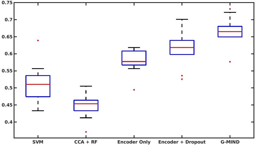
intuitive (i.e., equal importance is given to both the imaging and genetic data), and it is not performance driven
(i.e., we do not cherry-pick the values to optimize prediction accuracy). The corresponding values for all the
experiments are: λ1 = 0.1, λ2 = 0.1, λ3 = 0.01, λ4 = 0.1, and λ5 = 0.01. We fix the Bernoulli probability, to
q = 0.001 and the temperature variable to t = 0.1. Based on 10-fold cross validation results we fix all detection
threshold values to τi = 0.1. The architecture of our model (layer sizes and nonlinearities) is shown in Fig. 1.

2.7 Baseline Comparison Methods
We compare G-MIND to classical machine learning techniques and architectural variants that omit key features.

   • Multimodal Support Vector Machine (SVM): We construct a linear SVM classifier after concate-
     nating all the data modalities [iT1 , iT2 , gT ]T . Notice that this model cannot handle missing data. Therefore,
     we fit a multivariate regression to impute missing imaging modalities based on the available one for each
     subject. For example if in1 is absent, we impute it as: in1 = β ∗ in2 , where β is the regression coefficient matrix
     obtained from training data. We use a grid search method to find the best set of hyper-parameters. Notice
     that this tuning provides an added advantage for SVM over G-MIND.
   • Multimodal CCA + RF: Canonical correlation analysis (CCA) identifies bi-multivariate associations
     between imaging and genetics data. This approach is similar to our coupled latent projection, but the
     traditional CCA does not accommodate more than two data modalities. In order to overcome this we
     concatenate the imaging features obtained from two experimental paradigms and perform CCA with the
     genetics data. We then construct a random forest classifier based on the latent projections. We use the
     same approach for data imputation and to find the best set of hyperparameters.
   • Encoder Only: We compare our model to an ANN architecture based on the encoder and the classifier of
     G-MIND. This comparison will show us importance of using the decoder and the learnable dropout layer.
   • Encoder+Dropout: We compare our model to another ANN architecture where we only used the encoder,
     the classifier, and the learnable dropout layer. This experiment will show us the performance improvement
     from including a decoder. Based on our 10-fold cross validation we fix the learned dropout threshold values
     to {τi1 = 0.05, τi2 = 0.05, τg = 0.1}.

                                    3. EXPERIMENTAL RESULTS
3.1 Data and Preprocessing
Our first dataset includes two task fMRI paradigms and SNP data provided by Lieber Institute for Brain
Development (LIBD) in Baltimore, MD, USA. The first fMRI paradigm is a working memory task (Nback)
that alternates between 0-back and 2-back trial blocks. During the 0-Back task the subjects is asked to press a
number shown on the screen, and during the 2-back task the subjects are instructed to press the number shown 2
stimuli previously. The second fMRI paradigm is an event-based simple declarative memory task (SDMT) which
involves incidental encoding of complex visual scenes. Our replication dataset includes just Nback and SNP data
acquired at the University of Bari Aldo Moro, Italy (BARI). The distribution of the subjects is shown in Table 1.
All fMRI data was acquired on 3-T General Electric Sigma scanner (EPI, TR/TE = 2000/28 msec; flip angle
= 90; field of view = 24 cm, res: 3.75 mm in x and y dimensions and 6 mm in the z dimension for NBack and
5 mm for SDMT). FMRI preprocessing include slice timing correction, realignment, spatial normalization to an
MNI template, smoothing and motion regression. SPM12 is used to generate activation and contrast maps for
each paradigm. We use the Brainnetome atlas19 to define 246 cortical and subcortical regions. The input to our
model is the contrast map over these ROIs.
    In parallel, genotyping was done using variate Illumina Bead Chips including 510K/ 610K/660K/2.5M.
Quality control and imputation were performed using PLINK and IMPUTE2 respectively. The resulting 102K
linkage disequilibrium independent SNPs are used to calculate the polygenic risk score of schizophrenia via a
log-odds ratio of the imputation probability for the reference allele.20 By selecting P < 10−4 , we obtain 1242
linkage disequilibrium independent SNPs. As a preprocessing step, we remove the effect of age, IQ, and education
from the imaging modalities and we have mean centred all the data modalities.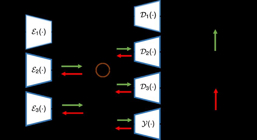
Perf
                        Sens   Spec   Acc     Auc
  Method
         SVM            0.66   0.47   0.58   0.55

       CCA+RF           0.15   0.92   0.51   0.56

      Encoder Only      0.57   0.57   0.57   0.59

   Encoder + Dropout    0.61   0.56   0.59   0.62

        G-MIND          0.75   0.58   0.67   0.68

Table 2: Testing performance of each method              Figure 3: Distribution of accuracies by the models
on LIBD during 10 fold cross validation.                 trained in all 10 CV folds, when directly evaluated on
                                                         BARI.

3.2 Model Performance
Table 2 quantifies the 10-fold testing performance of all the methods on multimodal data obtained from LIBD.
We can clearly see that G-MIND achieves the best overall accuracy. Even in the presence of missing data our
multi modal approach can successfully extract meaningful information from all the data modalities that are
essential for diagnosis prediction. Our results also show the importance of the decoder and the dropout layer.
    In order to show the generalizability of our method we trained our model on LIBD data and tested it without
fine tuning on a cross site dataset from BARI. This experiment captures the transference property of our model.
We note that the SDMT task was not acquired at BARI, so the corresponding branch of G-MIND is not used.
We evaluate the 10 best models obtained from the 10 different folds to run this experiment. Fig. 3 shows the
distribution of accuracies of all the models in the form of a boxplot. Here we can see that our method shows the
best transference property compared to all the baselines. This is an interesting result as it shows the robustness
of our model against data acquisition noise and population specific noise. This performance gain further suggests
that the learnable dropout mask can identify robust set of features that are most predictive of the disease.

3.3 Analysis of Imaging Biomarkers
Fig. 4 illustrates the most important set of brain regions as identified by the median concrete dropout probability
maps {pi1 , pi2 } across the 10 validation folds. We further show a more global picture of the high importance
brain regions as a surface plot in Fig. 5. Both from, Fig. 4 and Fig. 5 for the Nback task we can see
regions that include superior frontal gyrus (SFG),and inferior frontal gyrus (IFG), which are know to sub-serve
executive cognition.21 Moreover, we can see regions (SFG, IFG) from dorsolateral prefrontal cortex21 and regions
(SPL, STG) from posterior parietal cortex that overlaps with the fronto-parietal network which is known to be
altered in schizophrenia. Further clusters incorporate components of the default mode network also implicated in

Figure 4: The representative set of brain regions as captured by the dropout probabilities {p1 , p2 }. The color
bar denotes the median value across 10 folds.
Figure 5: The surface plot of the brain regions as captured by the dropout probabilities {p1 , p2 }. The color bar
denotes the median value across 10 folds. From Left to Right the images are internal surface of left hemisphere
(L–IN), external surface of left hemisphere (L–OUT), internal surface of right hemisphere (R–IN), and external
surface of right hemisphere (R–OUT).
schizophrenia.22 The SDMT biomarkers implicate the hippocampal, parahippocampal, superior frontal regions
along with the anteromedial thalamus which are also affected in schizophrenia.23 These regions control executive
cognition and memory encoding and that are also known to be associated with the disorder.
We further use Neurosynth24 to decode the higher order brain states of the the biomarkers associated with
Nback and SDMT tasks. This analysis allows us to quantitatively compare the selected brain regions with
previously published results and gives us a level of association with different brain states as identified by other
studies. Fig. 6 shows the Neurosynth terms that are strongly correlated with our biomarkers. We note that the
terms associated with the Nback task corresponds to recognition and solving while the brain states for SDMT
are associated with emotions and memory encoding. These results provide further evidence that G-MIND can
extract potential imaging biomarkers that are highly relevant to the task and the disorder under study.
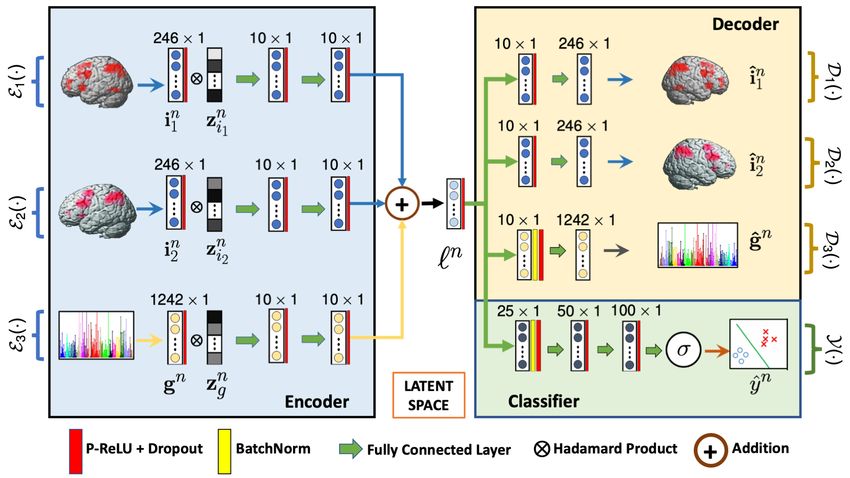
Fig. 7 shows the importance map across the 1242 SNPs as computed by the median pg across the 10 folds.
Figure 6: The level of association with different cognitive states of all the brain regions identified by our model
as found in the Neurosynth database.Biological Processes FDR
Central nervous system development 0.005
→ Nervous system development 0.001
→ System development. 0.005
Generation of neurons 0.005
→ Neurogenesis 0.004
Regulation of calcium ion
0.04
transport into cytosol
→ Regulation of sequestering of calcium ion 0.008
Figure 7: The median importance map of all the SNP Table 3: The enriched biological processes and their
across and their overlapping genes across the 10 folds. level of significance obtained via GO enrichment anal-
ysis.
We annotated each SNP based on its overlapping or nearest gene as found from the SNP-nexus web interface.25
In addition, we ran a gene ontology enrichment analysis of the overlapping genes of the top 300 SNPs to identify
the enriched biological processes.26 This enrichment analysis gives us a way to identify the set of over-represented
genes in a biological pathway that may have an association with the disease phenotype. Table 3 captures the most
significant biological processes implicated by the set of SNPs, which include the nervous system development,27
and calcium ion regulation 28 which are known to be strongly associated with schizophrenia. As parallel to
Neurosynth analysis, we perform a gene expression based analysis29 over the 10 overlapping (or nearest gene if
there is no overlap) genes of the top SNPs identified from our analysis. Here we use the GTEx database to identify
the set of brain tissues where these genes show high levels of expression. This exploratory analysis may help us
to understand the cis-effects of the SNPs and how they alter the functionalities of genes expressed in different
tissues of the brain. Figure 8 shows the gene expression pattern of each gene across different brain tissues. Here,
LINC00599 shows high expression levels in brain and are also known to be associated with schizophrenia30 and
neuroticism.31 These findings show that the model can be used to explore potential genetic biomarkers and their
interactions in a multivariate framework.
Figure 8: The gene expression pattern of the selected set of genes in different brain tissues based on the GTEx
database. Higher level of a gene expression in a brain tissue imply that alteration in that gene may have a
stronger effect on those specific brain regions.4. CONCLUSION
We have presented G-MIND, a novel deep network to integrate multimodal imaging and genetic data for targeted
biomarker discovery and class prediction. Our unique use of learnable dropout with a classification module helps
us to identify discriminative biomarkers of the disease. Our unique loss function enables us to handle missing
modalities while mining all the available information in the dataset. We demonstrate our framework on fMRI and
SNP data of schizophrenia patients and controls from two different sites. The improved performance of G-MIND
across all the experiments shows the capability this model to build a comprehensive view about the disorder
based on the incomplete information obtained from different modalities. We note that, our framework can easily
be applied to other imaging modalities, such as structural and diffusion MRI simply by adding autoencoder
branches. In future work we will develop a hybrid extension of G-MIND in which we incorporate pathway
specific information into the deep learning architecture for better understanding of the disease propagation.
Acknowledgements: This work was supported by NSF CRCNS 1822575, and the National Institute of Mental
Health extramural research program.
Previous Submission This work has not been published to any other publication venue.
REFERENCES
1. J. Zihl, G. Grön, and A. Brunnauer, “Cognitive Deficits in Schizophrenia and Affective Disorders: Evidence
for A Final Common Pathway Disorder,” Acta Psychiatrica Scandinavica 97(5), pp. 351–357, 1998.
2. C. Lee et al., “Prevention of Schizophrenia: Can It be Achieved?,” CNS Drugs 19(3), pp. 193–206, 2005.
3. S. Erk et al., “Functional Neuroimaging Effects of Recently Discovered Genetic Risk Loci for Schizophrenia
and Polygenic Risk Profile in Five RDoC Subdomains,” Translational Psychiatry 7(1), p. e997, 2017.
4. Wang et al., “Identifying Quantitative Trait Loci via Group-sparse Multitask Regression and Feature Se-
lection: An Imaging Genetics Study of The ADNI Cohort.,” Bioinformatics (Oxford, England) 28(2),
pp. 229–37, 2012.
5. J. Liu et al., “A Review of Multivariate Analyses in Imaging Genetics,” Frontiers in Neuroinformatics 8,
p. 29, 2014.
6. E. C. Chi et al., “Imaging Genetics via Sparse Canonical Correlation Analysis.,” Proceedings. IEEE Inter-
national Symposium on Biomedical Imaging 2013, pp. 740–743, 2013.
7. S. A. Meda et al., “A Large Scale Multivariate Parallel ICA Method Reveals Novel Imaging-genetic Rela-
tionships for Alzheimer’s Disease in The ADNI Cohort,” NeuroImage 60(3), pp. 1608–1621, 2012.
8. G. Pergola et al., “DRD2 Co-expression Network and a Related Polygenic Index Predict Imaging, Behavioral
and Clinical Phenotypes Linked to Schizophrenia,” Translational Psychiatry 7(1), p. e1006, 2017.
9. N. K. Batmanghelich et al., “Probabilistic Modeling of Imaging, Genetics and Diagnosis.,” IEEE transactions
on medical imaging 35(7), pp. 1765–79, 2016.
10. S. Ghosal et al., “Bridging Imaging, Genetics, and Diagnosis in a Coupled Low-dimensional Framework,”
in MICCAI: Medical Image Computing and Computer Assisted Intervention, 11767 LNCS, pp. 647–655,
Springer, 2019.
11. H. Kang, “The prevention and handling of the missing data,” Korean Journal of Anesthesiology 64(5),
pp. 402–406, 2013.
12. A. Ben Said, A. Mohamed, T. Elfouly, K. Harras, and Z. J. Wang, “Multimodal deep learning approach for
Joint EEG-EMG Data compression and classification,” in IEEE Wireless Communications and Networking
Conference, WCNC, Institute of Electrical and Electronics Engineers Inc., 2017.
13. D. P. Kingma and J. Ba, “Adam: A method for stochastic optimization,” CoRR abs/1412.6980, 2015.
14. N. Jaques et al., “Multimodal autoencoder: A deep learning approach to filling in missing sensor data
and enabling better mood prediction,” in 2017 7th International Conference on Affective Computing and
Intelligent Interaction, ACII 2017, 2018-January, pp. 202–208, Institute of Electrical and Electronics
Engineers Inc., 2018.15. Y. Gal et al., “Concrete Dropout,” in Advances in Neural Information Processing Systems 30, pp. 3581–3590,
Curran Associates, Inc., 2017.
16. Y. Gal and Z. Ghahramani, “Dropout as a bayesian approximation: Representing model uncertainty in deep
learning,” in international conference on machine learning, pp. 1050–1059, 2016.
17. E. Jang et al., “Categorical Reparameterization with Gumbel-Softmax,” 5th International Conference on
Learning Representations, ICLR 2017 - Conference Track Proceedings , 2016.
18. K. He et al., “Delving deep into rectifiers: Surpassing human-level performance on imagenet classifica-
tion,” in Proceedings of the 2015 IEEE International Conference on Computer Vision (ICCV), ICCV ’15,
p. 1026–1034, IEEE Computer Society, 2015.
19. L. Fan et al., “The Human Brainnetome Atlas: A New Brain Atlas Based on Connectional Architecture,”
Cerebral Cortex 26(8), pp. 3508–3526, 2016.
20. Q. Chen et al., “Schizophrenia Polygenic Risk Score Predicts Mnemonic Hippocampal Activity,”
Brain 141(4), pp. 1218–1228, 2018.
21. J. H. Callicott et al., “Abnormal fMRI Response of The Dorsolateral Prefrontal Cortex in Cognitively Intact
Siblings of Patients with Schizophrenia,” American Journal of Psychiatry 160(4), pp. 709–719, 2003.
22. F. Sambataro et al., “Treatment with Olanzapine is Associated with Modulation of The Default Mode
Network in Patients with Schizophrenia,” Neuropsychopharmacology 35(4), pp. 904–912, 2010.
23. R. Rasetti et al., “Altered Hippocampal-Parahippocampal Function During Stimulus Encoding,” JAMA
Psychiatry 71(3), p. 236, 2014.
24. W. Tor D., “NeuroSynth: a new platform for large-scale automated synthesis of human functional neu-
roimaging data,” Frontiers in Neuroinformatics 5, 2011.
25. A. Z. Dayem Ullah et al., “SNPnexus: assessing the functional relevance of genetic variation to facilitate
the promise of precision medicine,” Nucleic Acids Research 46, pp. 109–113, 2018.
26. Mi and others., “Protocol Update for Large-scale Genome and Gene Function Analysis with The PANTHER
Classification System (v.14.0),” Nature Protocols 14(3), pp. 703–721, 2019.
27. B. Dean, “Is Schizophrenia The Price of Human Central Nervous System Complexity?,” Australian and
New Zealand Journal of Psychiatry 43(1), pp. 13–24, 2009.
28. M. J. Berridge, “Dysregulation of Neural Calcium Signaling in Alzheimer Disease, Bipolar Disorder and
Schizophrenia,” in Prion, 7(1), pp. 2–13, Landes Bioscience, 2013.
29. J. Lonsdale et al., “The Genotype-Tissue Expression (GTEx) project,” 45(6), pp. 580–585, 2013.
30. F. S. Goes et al., “Genome-wide association study of schizophrenia in Ashkenazi Jews,” American Journal
of Medical Genetics Part B: Neuropsychiatric Genetics 168(8), pp. 649–659, 2015.
31. M. Luciano et al., “Association analysis in over 329,000 individuals identifies 116 independent variants
influencing neuroticism,” Nature Genetics 50(1), pp. 6–11, 2018.You can also read