Dynamics of Social Mobility during the COVID-19 Pandemic in Canada - IZA DP No. 13376 JUNE 2020

DISCUSSION PAPER SERIES

IZA DP No. 13376

Dynamics of Social Mobility during the
COVID-19 Pandemic in Canada

Mutlu Yuksel
Yigit Aydede
Francisko Begolli

JUNE 2020

DISCUSSION PAPER SERIES

IZA DP No. 13376

Dynamics of Social Mobility during the
COVID-19 Pandemic in Canada

Mutlu Yuksel
Dalhousie University and IZA
Yigit Aydede
Saint Mary’s University
Francisko Begolli
Dalhousie University

JUNE 2020

Any opinions expressed in this paper are those of the author(s) and not those of IZA. Research published in this series may
include views on policy, but IZA takes no institutional policy positions. The IZA research network is committed to the IZA
Guiding Principles of Research Integrity.
The IZA Institute of Labor Economics is an independent economic research institute that conducts research in labor economics
and offers evidence-based policy advice on labor market issues. Supported by the Deutsche Post Foundation, IZA runs the
world’s largest network of economists, whose research aims to provide answers to the global labor market challenges of our
time. Our key objective is to build bridges between academic research, policymakers and society.
IZA Discussion Papers often represent preliminary work and are circulated to encourage discussion. Citation of such a paper
should account for its provisional character. A revised version may be available directly from the author.

 ISSN: 2365-9793

 IZA – Institute of Labor Economics
Schaumburg-Lippe-Straße 5–9 Phone: +49-228-3894-0
53113 Bonn, Germany Email: publications@iza.org www.iza.org

IZA DP No. 13376 JUNE 2020

 ABSTRACT
 Dynamics of Social Mobility during the
 COVID-19 Pandemic in Canada
 As the number of cases increases globally, governments and authorities have continued to
 use mobility restrictions that were, and still are, the only effective tool to control for the
 viral transmission. Yet, the relationship between public orders and behavioral parameters
 of social distancing observed in the community is a complex process and an important
 policy question. The evidence shows that adherence to public orders about the social
 distancing is not stable and fluctuates with degree of spatial differences in information
 and the level of risk aversion. This study aims to uncover the behavioural parameters of
 change in mobility dynamics in major Canadian cities and questions the role of people’s
 beliefs about how contagious the disease is on the level of compliancy to public orders.
 Our findings reveal that the degree of social distancing under strict restrictions is bound by
 choice, which is affected by the departure of people’s beliefs from the public order about
 how severe the effects of disease are. Understanding the dynamics of social distancing thus
 helps reduce the growth rate of the number of infections, compared to that predicted by
 epidemiological models.

 JEL Classification: I20, I26, J24
 Keywords: COVID-19, mobility, transmission, viral infections

 Corresponding author:
 Mutlu Yuksel
 Department of Economics
 Dalhousie University
 6214 University Avenue
 Halifax, NS B3H 4R2
 Canada
 E-mail: mutlu@dal.ca

1. Introduction
 As the number of cases increases globally, governments and authorities have
 continued to use mobility restrictions that were, and still are, the only effective tool
 to control for the viral transmission. Centers for Disease Control and Prevention
 defines these public responses as Nonpharmaceutical Interventions (NPIs): “actions,
 apart from getting vaccinated and taking medicine, that people and communities
 can take to help slow the spread of illnesses like pandemic influenza (flu)”.4 There
 are recent studies (Chen and Qiu 2020, Zang et al. 2020, Fang et al. 2020)
 investigating how effective lockdown policies are by looking at the daily incidence
 of COVID19 and mobility patterns. Although the evidence unambiguously
 indicates that implementing NPIs with successful social distancing measures have
 the largest effect on curbing the pandemic, in a recent study, Askitas et al. (2020)
 find that restrictions on internal movement, public transport closures and
 international travel controls do not lead to a significant reduction of new infections.
 They explain that the reason of this limited impact of mobility restrictions is due
 to the lack of stringency in the policy implementations.
 As in any democratic system, the relationship between public orders and
 behavioral parameters of obedience to those orders observed in a community is a
 complex process and an important policy question. It is vital for public authorities
 to understand this relationship as well as how it manifests across time and regions.
 Mobility patterns show how effective the lockdown policies are to control for
 infectious disease spread. The evidence confirms that adherence to public orders
 about the social distancing is not stable and fluctuates with degree of spatial and
 temporal differences in information and the level of risk aversion. From a policy
 perspective, policy makers must understand the determinants of adherence to
 movement restrictions to analyze the efficacy of the public health orders in any given
 time and region, which will also help them prepare for the possible second wave of
 COVID19.5
 This study aims to uncover the behavioural parameters of change in mobility
 dynamics in major Canadian cities and questions the role of people’s beliefs about

4
 https://www.cdc.gov/nonpharmaceutical-interventions/index.html
5
 Studies that have looked at a possible second wave of COVID-19 include Leung et al (2020).
 2

how contagious the disease is on the level of compliancy to public orders.
Traditionally, studies examining mobility have ignored individual-level spatial and
temporal variation in where people spend time. More recently, these issues have been
addressed using the concept of an individual’s activity space (defined as
encompassing all the locations a person interacts with over time), yielding a much
more accurate picture of social mobility. In an effort to understand the COVID19
transmission due to movement, Google, Apple, and Facebook released their own
interfaces to explore how much mobility has been impacted as a result of the states
of emergencies that each province implemented. For instance, we show daily
changes in three mobility modes before and after mobility restrictions in Halifax in
Figure 1.

Figure 1: Apple Mobility Index - Halifax

Source: Authors’ own calculations using Apple Community Mobility Report data

 To the best of our knowledge, this is the first Canadian study that explores
aggregated city level mobility data. We attempt to uncover how mobility modes
such as daily changes in volumes of citizens using public transit have been impacted
due to public sentiments that reflect the people’s beliefs about how severe the effects
of disease are by examining variables such as the previous day's case and death

 3

count from COVID19. The study also controls for high-dimensional local weather
conditions and removes unobserved spatial heterogeneity across cities. Our findings
reveal that the degree of social distancing even under strict restrictions is bound by
choice, which is affected by the departure of people’s beliefs from the public order
about how grim the crisis is. Understanding the dynamics of social distancing thus
helps reduce the growth rate of the number of infections, compared to that
predicted by epidemiological models.
 The remainder of the paper is organized as follows: Section 2 introduces the data,
accompanying descriptive summaries, and illustrations; Section 3 reports the
estimation results and the discussions about the finding; and we provide the
concluding remarks in Section 4.

2. Data
There are three types of data that are prerequisites in this study: mobility measures,
local and high-dimensional weather metrics, and a proxy for a sentiment that
reflects how the pandemic compromises our emotional stability and results in
spatial and temporal deviance from or compliance with the public health order. All
the sources represent unconventional, high-dimensional, and dynamic data
structures with additional requirements for data management issues. The following
subsections will give the details of these data sources and illustrate the information
structures that each source offers.

2.1 Mobility Data
In April, regional mobility trends were made available for public use by Apple,
Google, and Facebook to aid COVID19 efforts. This is the first time in history that
one can publicly access the data covering different modes and levels of people’s
mobility in daily frequency for more than 131 countries and major cities. All three
providers commented on their websites that the availability of their data is
temporary for a limited time during the COVID19 pandemic. Apple's Mobility
Trends Report was released on April 14th by Apple, which is the main data source
used in this paper. Apple provides a csv file (wide form) directly downloadable

 4

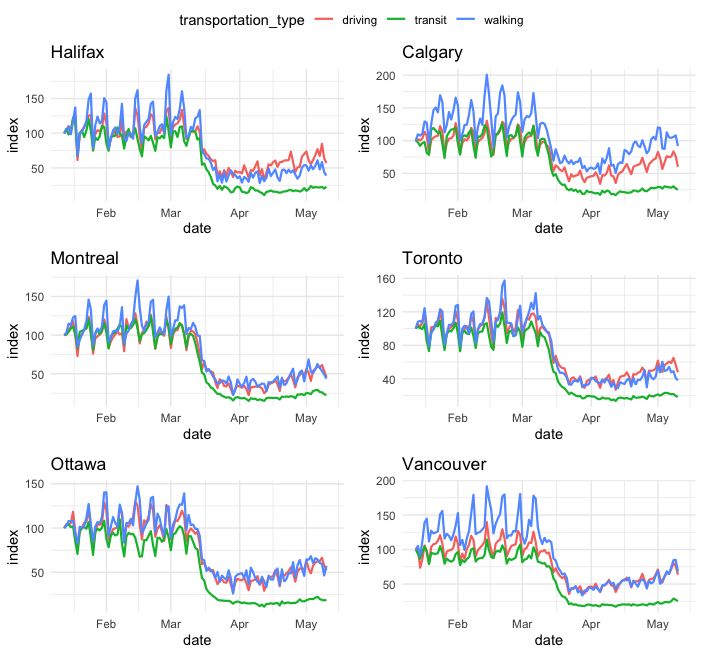
from their dedicated website starting from January 13, 2020.6 This anonymized
 data captures daily movement patterns across cities globally. The data provides
 the daily changes in volumes for driving, walking, and transit compared to the
 baseline volume indexed to 100 on the first date of observation (January 13) for a
 given mode of transport. The following six graphs shows the mobility trends for
 six cities.

 Figure 2: Apple Mobility Index – All Six Cities

 Source: Authors’ own calculations based on Apple Community Mobility data

6
 https://www.apple.com/covid19/mobility
 5

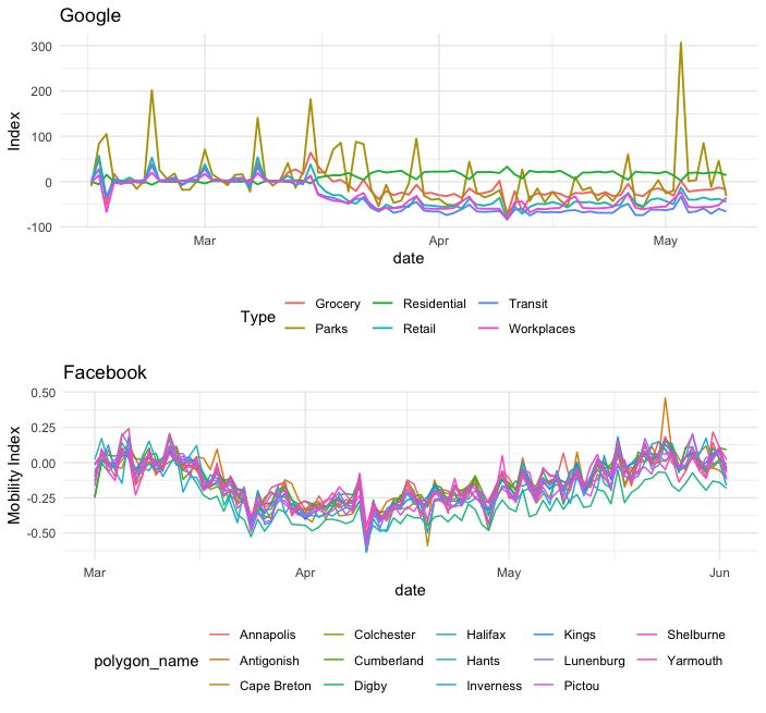
Google also provides regional Community Mobility Reports mobility trends to help
researchers look into predicting epidemics, plan urban and transit infrastructure,
and understand people’s mobility and responses to conflict and natural disasters.7
Although the data provide more detailed modes of mobility including retail, grocery,
parks, transit, workplaces and residential, Google does not provide disaggregated
city-level data for Canada. This level of aggregation at the provincial level masks
important geotemporal differences specially for larger provinces.

Figure 3: Google and Facebook – Nova Scotia

 Source: Authors’ own calculations based on Google and Facebook mobility data

7
 https://www.google.com/covid19/mobility/
 6

Finally, Facebook’s Movements Range Data is released in their website8
 stating that the data inform researchers and public health experts about how
 populations are responding to physical distancing measures. The Facebook data is
 the only data in finer spatial scales, at the county-level. Hence. the size of the data
 is big without any level of aggregation at the provincial level. These datasets have
 two different metrics: Change in Movement and Stay Put. The Change in
 Movement metric looks at how much people are moving around and compares it to
 a baseline period that predates most social distancing measures. The Stay Put
 metric looks at the fraction of the population that appears to stay within a small
 area surrounding their home for an entire day. We provide an illustration in Figure
 3 to give a better idea how Google and Facebook (Change in Movement) data look
 like.
 As it appears in these three mobility datasets, there is a trade-off between the
 level of information on mobility details and the level of spatial aggregation.
 Therefore, the ideal data for our work would be the Apple data with a city-level
 aggregation and just-enough details in mobility modes.

 2.2 Weather Data
 Although the historical climate data can be obtained from multiple sources, it
 requires a substantial amount of time and effort to select the right one. These
 sources compile the information based on physical weather stations located in
 different sections in the region. The most reliable data with minimum missing
 values are from stations that are located at the airports and many studies use their
 values for the cities. We have tried multiple data sources such as Climate Data
 Extraction Tool from the Government of Canada’s website9, and Air Quality
 Open Data Platform10, which provides a worldwide weather and air quality
 dataset specially organized for researches on the COVID-19 pandemic. Data
 collection is based on the physical weather stations located in different sections in
 the city. Because the most reliable data with minimum missing values are from
 stations that are located at the airports, we use their values for the cities. The

8
 https://data.humdata.org/dataset/movement-range-maps
9
 https://climate-change.canada.ca/climate-data/#/daily-climate-data
10
 https://aqicn.org/data-platform/covid19/verify/a1e436e6-5829-4b50-bfb3-82d2f4865d7c
 7

most reliable weather data, however, is provided at WeatherStats.ca.11 Their
 Weather Data Dashboard reports high-dimensional high-frequency data based
 on their own forecasting algorithms. Their data are collected over time from
 Environment and Climate Change Canada as well as Citizen Weather Observer
 Program (CWOP). The data contains 70 unique meteorological metrics for each
 city. The details are provided in Appendix.

 2.3 COVID-19 Data
 The data on COVID-19 for Canada was taken from the R package CanCovidData
 written by Von Bergmann (2020)12. We used the provincial data as a proxy for
 COVID-19 sentiment in major Canadian cities. Their data lines up with the official
 updates from the Public Health Agency of Canada. Table 1 below provides the
 most updated numbers for each province:

 Table 1: COVID-19 pandemic in Canada by province (June 13)
 Province Population Tests Cases Recov. Deaths Active
 British Columbia 5,110,917 165,256 2,709 2,354 168 187
 Alberta 4,413,146 325,149 7,346 6,811 159 346
 Saskatchewan 1,181,666 54,508 663 627 13 23
 Manitoba 1,377,517 55,255 301 289 7 5
 Ontario 14,711,827 953,015 31,726 26,187 2,498 3,041
 Quebec 8,537,674 515,673 53,666 20,823 5,148 27,695
 New Brunswick 779,993 36,125 154 125 1 28
 Prince Edward Island 158,158 8,463 27 27 0 0
 Nova Scotia 977,457 48,787 1,061 995 62 4
 Newfoundland and Lab. 521,365 14,256 261 256 3 2
 Canada 37,894,799 2,178,345 97,943 58,513 8,049 31,371
 Source: https://en.wikipedia.org/wiki/COVID-19_pandemic_in_Canada

 We are aware that a sentiment analysis at diverse temporal and spatial scales is
 not a simple task and the use of cases or deaths as a proxy for the local sentiment
 on COVID19 pandemic would be problematic. One of the essential issues is that

11
 https://www.weatherstats.ca
12
 https://mountainmath.github.io/CanCovidData/
 8

even if the number of cases or deaths rises, it would be possible to observe that the
 people’s feeling become positive. In a recent work, Yu et al.13 mine the Twitter
 data for the content of COVID-19 related tweets to see how people’s feelings and
 expressions changed over time during the pandemic in the U.S. Figure 4 below
 shows five segments of sentiment, one of which is fearfulness. As it is clear from
 the figure, even though the number of cases rises, people feel less fearful. In our
 estimations in the next section, we will comment on this fact.

 Figure 4: Segments of Sentiment in the U.S due to COVID19 Pandemic

 Source: https://public.tableau.com/profile/nanluo#!/vizhome/Book2_v2_15887433980520/SentimentLevel

 3. Empirical framework and estimation results
 3.1 Framework
 Our empirical objective is to explore the sensitivity of the social mobility to local
 weather conditions and sentiment that reflects the people’s feeling about beliefs on
 how contagious the disease is. Since the state of emergency rules do not change
 day by day, any significant effect of the weather conditions as well as the sentiment

13
 https://github.com/xxz-jessica/COVID-19_UCD_Challenge
 9

that is captured by the lag values of pervious COVID19 cases (or deaths) on the
 local social mobility demonstrate the degree to which people’s choice departs from
 the public order.
 After merging all three data sources, we obtain an unbalanced long panel with
 six cities and about 420 observations between March 1 and May 10. Due to time
 dimension of the data, we applied several panel unit root tests (Breitung and
 Pesaran, 2008), and none of them indicated the existence of a unit root.
 We start our analysis by estimating the determinants of the mobility
 discussed in data section. In these estimations, we utilize the pooled OLS, fixed
 effect and random effect models. These estimates further help us to calculate the
 weather elasticity of mobility, and sentiment elasticities of mobility. More
 specifically, we first estimate the following regression using pooled OLS for city i in
 a given day t:

 = + 1 −1 + 2 ℎ + + + (1)

 where ℎ is a vector of seventy different measures of weather conditions listed
 in Appendix. We define our outcome variable, , separately in
 specification as transit, driving, and walking from the Apple data. In order to
 capture an overall mobility index, we also use two average values. First, since
 driving and transit indices generally move in opposite directions, they may cancel
 out each other. Therefore, the average of driving and transit may capture the
 overall daily mobility within the city. Second, we also use the total mobility, which
 is defined as the average of three modes of mobility. As for sentiments towards
 COVID19 in each city and day, we use the daily numbers of new deaths and new
 cases from the previous day, which is denoted by −1 .Using the values
 from the previous day allows for the potential delays in announcements by health
 and provincial authorities. We control for city dummies, ! to account for the
 unobserved heterogeneity across cities. Finally, as illustrated in the graphs, all
 mobility measures exhibit cyclical daily trends. Hence, we control for these trends
 by adding day of the week dummies, .14

14
 We also tested time fixed effects for each day. Their addition does not improve the results, which
are also rejected by a simple F-test.
 10

As it is an ad-hoc empirical model, Specification (1) can be extended by the
 choice of variables and the introduction of nonlinearity with different levels of
 polynomials and interactions. In order to find the most explanatory weather
 variables among seventy different metrics, we applied penalized regression methods
 (LASSO) to reduce the high dimensionality in Specification (1). At the end of the
 process, very few weather variables are chosen as significant predictors. We used
 these variables as our base set and expanded it with different specifications. As for
 the nonlinearity, we applied several different non-parametric models (mostly
 ensemble learning algorithms and TensorFlow applications) and compared their
 predictive powers with the base and extended models. The results indicate that
 linear models with the selected weather variables can capture the essence of
 relationship between mobility metrics and the selected covariates.15
 After these estimations, we calculated the average marginal effect of weather
 and sentiments at the means of other variables. Using these average marginal
 effects, we calculated the elasticity of daily cases of transit, driving, and walking.
 In a similar way, we calculated elasticity of temperature, and precipitation of
 mobility, and each city as well. Moreover, we calculated marginal elasticities at
 different level of sentiments, and weather conditions.

 3.2 Results
 We begin by estimating a fixed-effect model given in Equation (1) by using a
 dummy variable least square method. The objective of this estimation to
 investigate the association between the factors abstracted in the previous sections
 and the mobility of the local population within a city. The estimation results for
 each mobility mode are summarized in Table 2. For each mobility model, we define
 three specifications starting from a base model with maximum temperature and
 add precipitation amount and the minimum wind speed in the second and third
 specifications, respectively.

15
 The results of LASSO and nonparametric estimations and their scripts can be provided upon request.
 11

Table 2. Estimations of transportation modes within city
 Variables Transit Driving Walking
 (1) (2) (3) (4) (5) (6) (7) (8) (9)

 Cases -0.03** -0.03** -0.03** -0.03** -0.03** -0.03** -0.03** -0.03** -0.03**
 (0.00) (0.00) (0.00) (0.00) (0.00) (0.00) (0.00) (0.00) (0.00)
 Temperature -1.03** -1.02** -1.05** -0.18 -0.18 -0.20 0.04 0.06 0.02
 (0.21) (0.20) (0.21) (0.18) (0.17) (0.18) (0.24) (0.23) (0.24)
 Precipitation -0.49* -0.44 -0.55** -0.50* -0.92** -0.84**
 (0.20) (0.23) (0.17) (0.19) (0.22) (0.25)
 Wind speed -0.18 -0.18 -0.27
 (0.29) (0.26) (0.34)
 Observations 420 420 420 420 420 420 420 420 420
 R-squared 0.28 0.29 0.29 0.26 0.27 0.27 0.29 0.31 0.31
Robust standard errors clustered at the city-level are in parenthesis. Significance levels are (**) is p < 0.01 and (*) is p
< 0.05. All specifications include city and day-of-week fixed effects. Cases represents the number of previous day’s new
COVID19 cases. Temperature measures the daily maximum temperature. Wind speed represents the daily minimum wind
speed value. Precipitation is the daily total precipitation level.

 The findings in columns (1-3) in Table 2 are consistent with expectations that the
 use of public transportation decreases when the number of COVID19 cases rises.
 Our results also indicate that the transit usage decreases when daily temperature
 increases. Similarly, an increase in precipitation also leads to a decline in the
 utilization of transit. However, wind does not have any statistical effect on transit
 usage.
 In the following columns of Table 2, we further analyze the effect of the same
 factors on driving. We again find that a rise in COVID19 cases and more
 precipitation decreases the likelihood of driving. However, our results indicate that
 temperature does not have any effect on driving within a city. Similarly, in
 Columns (6-9), we show that cases and precipitation decrease walking, while
 temperature does not seem to be affecting the individual’s decision to walk.
 We next turn to investigate whether the combination of indexes, which could
 be a better measure of overall mobility, will yield different findings. The results
 are summarized in Table 3. In Columns (1-3), our main outcome for mobility is
 the average of transit and driving indices. A strong negative correlation between
 driving and transit during the pandemic indicates that people switch their mode of
 transportation without necessarily cutting back their overall mobility. Therefore,

 12

averaging these two modes would provide a better index to measure the variation
in social mobility. Following the same reasoning, in Columns (4-6), the main
outcome is the average of three modes we used in our analyzes. Mainly, we are
interested in capturing whether these modes of mobility act as substitutes or the
changes in the local weather and sentiment affect people’s overall mobility. Our
results reveal that the number of cases, temperature, and precipitation lead to a
decline in overall driving and transit use within a city. However, the effect of
temperature becomes less robust when we include all transportation modes, which
may indicate that people substitute using transit and cars with walking when the
temperature increases.

Table 3. Estimations of mobility index within city
 Variables Average of Driving + Transit Average of all modes
 (1) (2) (3) (4) (5) (6)
 Cases -0.03** -0.03** -0.03** -0.03** -0.03** -0.03**
 (0.00) (0.00) (0.00) (0.00) (0.00) (0.00)
 Temperature -0.61** -0.60** -0.62** -0.39 -0.38 -0.41*
 (0.19) (0.19) (0.19) (0.20) (0.20) (0.20)
 Precipitation -0.52** -0.47* -0.65** -0.59**
 (0.18) (0.21) (0.19) (0.22)
 Wind speed -0.18 -0.21
 (0.27) (0.29)
 Observations 420 420 420 420 420 420
 R-squared 0.26 0.27 0.27 0.25 0.27 0.27
Robust standard errors clustered at the city-level are in parenthesis. Significance levels are (**) is p < 0.01
and (*) is p < 0.05. All specifications include city and day-of-week fixed effects. Cases denotes the number of
previous day’s new COVID19 cases. Temperature measures the daily maximum temperature. Wind speed
represents the daily minimum wind speed value. Precipitation is the daily total precipitation level.

 After examining what factors are significantly associated with the modes of
mobility, we also quantify their impact. One convenient way to understand the
magnitude of their effects is the elasticity of different modes of mobility with respect
to weather and sentiment. More specifically, we show the percentage change of
mobility when each factor changes by 1 percent.

 13

In Table 4, we present the overall factor elasticities of different modes of
 mobility. All these elasticities are calculated using the most comprehensive
 specifications, which are the last columns of each modes of mobilities, presented in
 Table 2 and Table 3. Moreover, all these elasticities are calculated at the mean
 values of each control variable. In Column (1), we show that the elasticity of daily
 cases is -0.31, and the elasticity of the temperature is -0.25, and the elasticity of
 the precipitation is -0.03. Taken together, these elasticities demonstrate that each
 1% increase in the number of cases in the previous day leads to a decline in the
 transit usage by 0.3%. To capture sentiments, we also use an alternative measure,
 the number of deaths in the previous deaths. The results are very similar as
 expected as cases and deaths are highly correlated. The correlation between these
 two measures are 0.86 and cannot be used in the same estimation. We present these
 results in appendix table 1 and 2.

 Table 4. Elasticity of mobility modes
 Variables Transit Driving Walking Mobility1 Mobility2
 (1) (2) (3) (4) (5)

 Cases -0.32** -0.14** -0.17** -0.21** -0.19**
 (-0.04) (-0.02) (0.02) (0.03) (0.02)
 Temperature -0.26** -0.03 0 -0.11** -0.07*
 (-0.05) (0.03) (0.01) (0.04) (0.01)
 Precipitation -0.03 -0.02* -0.03** -0.02* -0.03
 (-0.01) (0.00) (0.00) (0.03) (0.03)
Robust standard errors are in parenthesis. **p

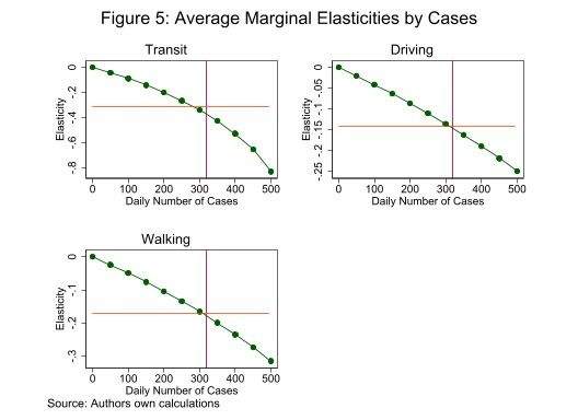
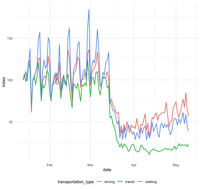
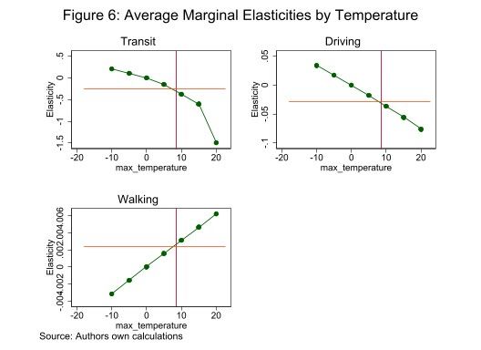
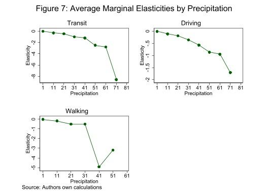
the extent of walking has not decreased too much in Calgary as it was not that
high to begin with. All these indexes averages are around 100 before closures, and
we present a detailed information on each index by city in Figure 2 above.
Meanwhile, during the same period, the average number of cases was 320,
temperature was 8.5 Celsius and precipitation was 2.2mm on average.
 Using these values and elasticities presented in Column (1) of Table 4, we
calculate the magnitudes in a more useful way for policy makers. When a given city
has 10 more cases than average, transit usage decreases approximately by 1%.
When temperature increases by 1Celsius than its average,8.5C, the transit decreases
by 3%. When precipitation increases by 1mm, then transit decreases 1.4%.
 In Figure 5, we present the daily number of previous cases’ elasticity of
different modes of transport. The horizontal lines represent the elasticity at the
average value of variables, which are the coefficients in Table 4, while the vertical
lines illustrate the average number of cases, which is used to calculate the
aforementioned elasticities. As known, elasticities could be different over the
varying number of cases. Alluding to this, we find in Figure 5 that the elasticity
for each type of mobility significantly decreases when there is an upsurge in the
number of cases.
 In a similar way, Figure 6 demonstrates the temperature elasticities of transit,
driving and walking at different level of temperatures. We find in Figure 6 that the
elasticity of transit usage and driving is very conducive to the changes in
temperature, where the intensity of both modes of transportation plunge with rising
temperatures. Interestingly, the elasticity of walking is increasing with higher levels
of temperature, and it turns to be positive when temperature is above 5 Celsius.
Moreover, from figure 6, we clearly observe that when weather gets warmer people’s
tendency for walking also significantly rises as well.
 Finally, the precipitation elasticity of mobility is illustrated in Figure 7. As
evident from the figure, these elasticities are negative and very small in magnitude
when there is a light precipitation, less than 4mm. However, we also see in Figure
7 that all different types of mobility were affected negatively and substantially
when precipitation amount exceeds 5mm.

 15

16

4. Conclusion
The COVID19 outbreak has been recorded in more than 200 countries with several millions
of confirmed cases and around seven percent mortality rate. In the later stages of the
epidemic, after failing to “trace” each infection back to its origin, nonpharmaceutical
interventions - commonly referred as “social distancing” or “lockdown” policies - were
undertaken. The aim of these interventions was to slow down the pandemic by limiting the
level of mobility and to keep health system capacities serviceable. Mobility restrictions
were, and still are, the only effective tool to control for the viral transmission.
 Although the evidence unambiguously indicates that implementing NPI’s with
successful social distancing measures have the largest effect on curbing the pandemic, they
do not lead to a significant reduction of new infections due to the lack of stringency in the
policy implementations. The adherence to public orders about the social distancing is not
stable and fluctuates with degree of spatial differences in information and the level of risk
aversion. Understanding the dynamics of social distancing thus helps reduce the growth
rate of the number of infections, compared to that predicted by epidemiological models.
 This study aims to uncover the behavioural parameters of change in mobility
dynamics in major Canadian cities and questions the role of people’s beliefs about how
contagious the disease is on the level of compliancy to public orders. We attempted to
uncover how mobility modes have been impacted due to public sentiments as well as

 17

weather conditions. The panel structure of the data allowed us to remove unobserved
spatial heterogeneity across cities so that our findings reveal how the degree of social
distancing measured by three modes of mobility are associated with their major
determinants.
 All results indicate that the sentiment proxied by the number of daily COVID19
cases has a strong impact on all modes of mobility. Among the seventy different weather
metrics, we find only three variables, temperature, precipitation, and wing speed, have
significant effects on the level of local mobility. Moreover, we document sizable elasticities
of mobility modes with respect to case numbers, temperature and precipitation suggesting
that individual's mobility decision indeed is conducive to these factors. Thereby, the future
public health interventions could potentially incorporate such responses in the design of
their policies. Our results further allude to varying elasticities between modes of
transportation and factors contributing these decisions depending on their levels. More
specifically, we find that elasticities for each mode of transportation increases by an
increasing COVID19 cases, temperature, and precipitation.

References

Apple (2020) “Apple’s Mobility Trend Reports” Retrieved June 13, 2020.
https://www.apple.com/covid19/mobility/.

Askitas, N.,T. Konstantinos, B. Verheyden. 2020. “Lockdown Strategies, Mobility
Patterns and Covid-19”. IZA Discussion Paper No. 13293.

Breitung, J. and M. H. Pesaran. 2008. “Unit roots and cointegration in panels. In L.
Matyas and P. Sevestre” (Eds.), The Econometrics of Panel Data (Third ed.). Springer-
Verlag.

Canadian Centre for Climate Services (2020), GitHub repository:
https://github.com/ECCC-CCCS

Centers for Disease Control and Prevention. "Nonpharmaceutical Interventions".
Retrieved June 13, 2020. https://www.cdc.gov/nonpharmaceutical-interventions/index.html

Chen, X., and Qiu, Z. 2020. Scenario analysis of non-pharmaceutical interventions on
global COVID-19 transmissions. COVID Economics. 1(7): 46-67.

COVID-19 pandemic in Canada. (2020, June 10). Retrieved June 13, 2020
 18

https://en.wikipedia.org/wiki/COVID-19_pandemic_in_Canada

Fang, H., Wang, L., & Yang, Y. 2020. “Human Mobility Restrictions and the Spread of
the Novel Coronavirus (2019-nCoV) in China”. SSRN Electronic Journal.
doi:10.2139/ssrn.3559382

Google LLC (2020) “Google COVID-19 Community Mobility Reports.” Retrieved June
13, 2020. https://www.google.com/covid19/mobility/

Jens von Bergmann, CanCovidData, (2020), Gihub repository,
https://mountainmath.github.io/CanCovidData/index.html

Leung, K., Wu, J. T., Liu, D., & Leung, G. M. 2020. “First-wave COVID-19
transmissibility and severity in China outside Hubei after control measures, and second-
wave scenario planning: a modelling impact assessment”. Lancet (London, England)
395(10233),1382– 1393. doi.org/10.1016/S0140-6736(20)30746-7

Luo, N. (2020, May 06). Twitter Sentiment Analysis during COVID-19. Retrieved June
13, 2020. https://public.tableau.com/profile/nanluo

The World Air Quality Index project. (n.d.). COVID-19 Worldwide Air Quality data.
Retrieved June 13, 2020 https://aqicn.org/data-platform/covid19/verify/a1e436e6-5829-
4b50-bfb3-82d2f4865d7c

University of California, Davis, COVIC-19_UCD_Challenge, GitHub repository,
https://github.com/xxz-jessica/COVID-19_UCD_Challenge

Weatherstats.ca based on Environment and Climate Change Canada data Retrieved June
13, 2020 https://www.weatherstats.ca/

Zhang, Chi and Chen, Cai and Shen, Wei and Tang, Feng and Lei, Hao and Xie, Yu and
Cao, Zicheng and Tang, Kang and Bai, Junbo and Xiao, Lehan and Xu, Yutian and Song,
Yanxin and Chen, Jiwei and Guo, Zhihui and Guo, Yichen and Wang, Xiao and Xu, Modi
and Zou, Huachun and Shu, Yuelong and Du, Xiangjun, Impact of Population Movement
on the Spread of 2019-nCoV in China (2/26/2020). Available at SSRN:
https://ssrn.com/abstract=3546090 or http://dx.doi.org/10.2139/ssrn.3546090

 19

Appendix

Table A.1 Effect of different factors on modes of transportation within city
 Variables Transit Driving Walking
 (1) (2) (3) (4) (5) (6) (7) (8) (9)
 Deaths -0.18** -0.18** -0.18** -0.09** -0.10** -0.10** -0.15** -0.16** -0.16**
 (0.03) (0.03) (0.03) (0.03) (0.03) (0.03) (0.03) (0.03) (0.04)
 Temperature -1.25** -1.23** -1.27** -0.43* -0.41* -0.45* -0.22 -0.19 -0.24
 (0.21) (0.21) (0.22) (0.18) (0.18) (0.19) (0.25) (0.24) (0.25)
 Precipitation -0.47* -0.40 -0.52** -0.45* -0.90** -0.80**
 (0.21) (0.24) (0.17) (0.20) (0.22) (0.26)
 Wind speed -0.24 -0.24 -0.33
 (0.32) (0.28) (0.36)
 Observations 414 414 414 414 414 414 414 414 414
 R-squared 0.17 0.17 0.18 0.15 0.16 0.16 0.20 0.22 0.22
Robust standard errors are in parenthesis. **p

Table A.3 : List of Weather Variables
 maximum temperature heating degree days
 average hourly temperature cooling degree days
 average temperature growing degree days base 5
 minimum temperature growing degree days base 7
 maximum humidex growing degree days base 10
 minimum windchill precipitation
 maximum relative humidity rain
 average hourly relative humidity snow
 average relative humidity snow amount on ground (cm)
 minimum relative humidity time of sunrise
 maximum dew point time of sunset
 average hourly dew point amount of daylight
 average dew point sunrise forecast
 minimum dew point sunset forecast
 maximum wind speed minimum UV forecast
 average hourly wind speed maximum UV forecast
 average wind speed minimum high temperature forecast
 minimum wind speed maximum high temperature forecast
 maximum wind gust minimum low temperature forecast
 wind gust direction speed maximum low temperature forecast
 maximum sea pressure solar radiation
 average hourly sea pressure maximum cloud cover 4 oktas
 average sea pressure average hourly cloud cover 4 oktas
 minimum sea pressure average cloud cover 4
 maximum station pressure minimum cloud cover 4
 average hourly station pressure maximum cloud cover 8 oktas
 average station pressure average hourly cloud cover 8 oktas
 minimum station pressure average cloud cover 8
 maximum visibility minimum cloud cover 8
 average hourly visibility maximum cloud cover 10 oktas
 average visibility average hourly cloud cover 10 oktas
 minimum visibility average cloud cover 10
 maximum health index minimum cloud cover 10
 average hourly health index
 average health index
 minimum health index
Source: https://www.weatherstats.ca/

 21