Multiple-Fault, Slow Rupture of the 2016 Mw 7.8 Kaikoura, New Zealand, Earthquake: Complementary Insights from Teleseismic and Geodetic Data
←
→
Page content transcription
If your browser does not render page correctly, please read the page content below
Bulletin of the Seismological Society of America, Vol. XX, No. XX, pp. –, – 2018, doi: 10.1785/0120170285

               Multiple-Fault, Slow Rupture of the 2016 M w 7.8 Kaikoura,
                   New Zealand, Earthquake: Complementary Insights
                          from Teleseismic and Geodetic Data
                                         by Yi-Ying Wen, Kuo-Fong Ma,* and Bill Fry

                   Abstract      We investigate the complex rupture properties of the 2016 M w 7.8
                   Kaikoura earthquake by jointly inverting teleseismic body-wave and regional Global
                   Positioning System (GPS) coseismic deformation data within a multifault model. We
                   validate our results by forward modeling recorded Interferometric Synthetic Aperture
                   Radar (InSAR) interferograms. Our study reveals the complementary depth-
                   dependent contributions of teleseismic and local geodetic data to the cumulative slip
                   distribution. The resulting joint inversion model of the rupture process and slip pattern
                   explains both the far-field (teleseismic data) and near-field (GPS and InSAR data)
                   observations. The model highlights variable rupture velocity throughout the sequence,
                   with an initial high-velocity (2:25 km=s) pulse followed by slow (∼1:5 km=s) yet
                   significant reverse and transverse motion on faults stretching at least 160 km to the
                   north of the origin. We map significant thrust motion on a dipping plane representing
                   the combined effects of the Hope, Hundalee, and Jordan thrust faults as well as large
                   strike-slip motion along the Kekerengu and Needles faults. The mainshock also
                   ruptured the deep portion of the subduction interface at a velocity of 1:0 km=s.

                            Introduction
     On 13 November 2016, the M w 7.8 Kaikoura earthquake                    delays of about 58 s from the W-phase solution, indicating that
struck the northeastern coast of the upper South Island,                     the 2016 Kaikoura mainshock cannot be well represented by a
New Zealand. The epicenter determined by New Zealand’s geo-                  single point source and may involve multiple rupture planes or
logical hazard monitoring center (GeoNet) was at 42.69° S,                   slip vector variations. Multifault rupture is evident in the geo-
173.02° E, with a focal depth of 15 km (Fig. 1). The earthquake              detic and field observations. These data show that at least 12
caused widespread strong ground motion, generating numerous                  faults, possibly including the southern Hikurangi subduction in-
landslides and damage to the built environment. Fortunately, it              terface, were involved in the mainshock sequence and extend
occurred in a sparsely populated area, limiting its societal im-             from the hypocenter in the south with the rupture length of
pact. The earthquake also generated tsunami waves up to                      ∼170 km northeastward to the Kekerengu fault (Litchfield et al.,
>5 m along the Kaikoura coast. The mainshock occurred in                     2016; Hamling et al., 2017; Kaiser et al., 2017).
the tectonically active and structurally complex plate boundary                   Several studies suggest that this complex earthquake
between the Pacific and Australian plates. The region marks the              involved rupture of both upper crustal faults and the subduc-
transition between the Hikurangi subduction zone to the north                tion megathrust (e.g., Bai et al., 2017; Duputel and Rivera,
and the transpressional dextral Alpine fault to the south.                   2017; Hamling et al., 2017). Previous studies have demon-
     According to the Global Centroid Moment Tensor (CMT)                    strated the weaknesses of investigating the source properties
solution (strike 219°, dip 38°, rake 128°; see Data and Resour-              of large earthquakes with a single type of data (Wen and Ma,
ces), the strike is consistent with the regional geological struc-           2010; Wen et al., 2012). Source models resulting from
tures, however, the dip angle is much shallower than the dip                 previous studies of the Kaikoura earthquake that utilized indi-
angles of the faults previously mapped in the region (Litchfield             vidual datasets (e.g., local geodesy, regional strong motion, or
et al., 2014, 2016). In addition, the Global CMT solution sug-               teleseismic long-period [LP] seismic data) have in many cases
gests an oblique thrust-faulting mechanism with a significant                been incompatible with one another; studies based on local
non-double-couple component of 43% and large centroid time                   and regional data generally map most source deformation
                                                                             to crustal faults (e.g., Hamling et al., 2017; Kaiser et al., 2017)
  *Also at Earthquake Disaster & Risk Evaluation and Management              whereas those based on teleseismic data attribute most defor-
(E-DREaM) Center, National Central University, Taoyuan City 32001, Taiwan.   mation to a megathrust-like source (e.g., Bai et al., 2017). On

                                                             BSSA Early Edition / 1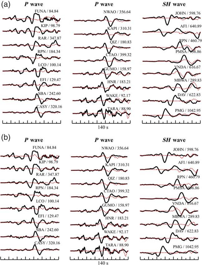
2                                                                                                        Y.-Y. Wen, K.-F. Ma, and B. Fry

                                                                                            GPS deformation field from our slip model
                                                                                            resulting from teleseismic only inversion.
                                                                                            We use the difference from this synthetic
                                                                                            GPS forward calculation and the observed
                                                                                            GPS measurements to decompose the con-
                                                                                            tribution of slip at deep and shallow depths
                                                                                            of the fault from the slip models. We exam-
                                                                                            ine our preferred model by forward model-
                                                                                            ing a synthetic InSAR interferogram, which
                                                                                            often better constrains broader regional
                                                                                            crustal deformation due to the advantage of
                                                                                            both its high resolution and wide coverage.
                                                                                            We find a good correlation between the syn-
                                                                                            thetic interferograms from our joint inver-
                                                                                            sion result and measured interferograms.

                                                                                                          Fault Geometry
                                                                                                    Field investigations show that the
                                                                                              2016 Kaikoura mainshock ruptured multi-
                                                                                              ple faults with many short segments, which
                                                                                              have various orientations and slip vectors
                                                                                              (Litchfield et al., 2016, 2017; Hamling
                                                                                              et al., 2017; Kaiser et al., 2017). The multi-
                                                                                              ple point-source model of Duputel and
                                                                                              Rivera (2017) suggests a southern strike-
                                                                                              slip fault with higher dip angle near the epi-
                                                                                              center, and both an oblique thrust as well as
Figure 1. Location of the 2016 Kaikoura earthquake and surrounding faults. Dots               a northern strike-slip fault with lower dip
indicate relocated aftershocks, recorded, and postprocessed with hypoDD by GNS Sci-           angles. Considering the resolution of tele-
ence, within 1 month after the mainshock. Dashed rectangles show the locations of three       seismic data, we adopt a simplified finite-
fault segments. Triangles represent the Global Positioning System (GPS) stations used in
this study. The color version of this figure is available only in the electronic edition.     fault geometry based on the previous stud-
                                                                                              ies, the field observations, and aftershock
                                                                                              distribution (Litchfield et al., 2016, 2017;
the other hand, Cesca et al. (2017) and Wang et al. (2018)               Duputel and Rivera, 2017; Hamling et al., 2017; Kaiser et al.,
proposed a model by jointly inverting Global Positioning                 2017). Therefore, as shown in Figure 1, two fault segments are
System (GPS), Interferometric Synthetic Aperture Radar                   set to correspond to the main geological structure with large
(InSAR), strong-motion, and teleseismic data.                            surface offsets (Litchfield et al., 2016, 2017; Hamling et al.,
      The 2016 Kaikoura earthquake was well recorded by                  2017; Kaiser et al., 2017). The first segment (F1), which was
global teleseismic stations. Teleseismic data typically have high        slightly adjusted from the strong-motion analysis (Kaiser et al.,
signal-to-noise ratios and widespread azimuthal coverage.                2017) to represent the rupture initiation on the Humps fault, is
Thus, they are frequently used to investigate the primary char-          an 80-km southern segment oriented N236°E with a 45-km
acteristics of fault rupture behavior and slip pattern. However,         width (i.e., down-dip extent) dipping 61°. Both the far-field
both their LP nature limit their sensitivity to small-scale com-         and near-field seismic data (Duputel and Rivera, 2017; Kaiser
plexities of the rupture process. Conversely, the static nature of       et al., 2017) suggest oblique faulting with a dip of 49° on the
near-field GPS and InSAR coseismic deformation data provides             northern part, which is consistent with the field observations
good constraints on the shallow-faulting pattern as well as the          (Litchfield et al., 2017). Although the dip angle of the Needles
total rupture area. These complementary sensitivities allow joint        fault is high, the coseismic offsets were much smaller than that
studies of teleseismic and local geodetic data to define rupture         of the Jordan thrust and Kekerengu faults. Thus, the second
models containing both small- and large-scale features. Signifi-         segment (F2) is represented as a 160-km northern segment
cantly, using joint inversion techniques, it is also possible to         oriented N225°E with a 55-km width dipping 49° to generally
map variations in rupture speed that might not be captured               represent the main energy released on the Jordan thrust and
by a single seismic type of dataset in isolation. In this study,         Kekerengu faults. In addition, several studies show that the
we resolve the spatial slip distribution from teleseismic and geo-       2016 Kaikoura earthquake released seismic moment on the
detic data. In addition to invert the spatial slip distribution from     subduction plate interface during the faulting (e.g., Bai et al.,
individual and joint dataset, we further calculate the synthetic         2017; Duputel and Rivera, 2017; Hamling et al., 2017; Wang
                                                          BSSA Early Edition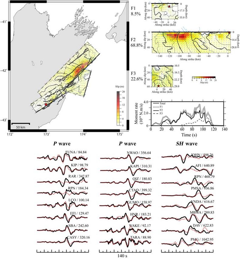
Multiple-Fault, Slow Rupture of the 2016 Kaikoura Earthquake                                                                                                                     3

                                                                            a regional 1D velocity structure modified from Eberhart-Phillips
                                                                            and Bannister (2010) and Fry et al. (2014). We invert coseismic
                                                                            offsets from 76 GPS stations within the study area (Fig. 1). In
                                                                            addition, we calculate the static ground displacements within the
                                                                            study area at every node of a 2 × 2 km grid to test our model
                                                                            against measured InSAR interferograms.
                                                                                 For a given seismic station, the displacement record can
                                                                            be represented as the linear sum of slip contributed from each
                                                                            ruptured subfault. Therefore, the observed and synthetic
                                                                            waveforms can be expressed as a system of linear equations:

                                                                                                     wA            wb
                                                                                                            x                           1
                                                                                                     λH             0
                                                                                                                                        EQ-TARGET;temp:intralink-;df1;313;613

                                                                            (Lee et al., 2013), in which A represents the matrix of
                                                                            Green’s functions of teleseismic waveforms and static
                                                                            ground displacements, b is the vector of observed data,
                                                                            and x is the solution matrix of the subfault dislocations.
                                                                            To ensure appropriate contributions from the different data-
                                                                            sets with different units and numbers of data points, we nor-
                                                                            malize the
                                                                                     P weight according to the following equations:
                                                                            w  1= jobserved data valuej=number of data. In addi-
Figure 2. Teleseismic station distribution. The star indicates the
epicenter of the 2016 Kaikoura earthquake. Triangles and squares            tion, H represents the stability constraint matrix, for exam-
represent the stations that recorded P- and SH-wave waveforms, re-          ple, the smoothing on the slip between adjacent subfaults,
spectively, used in this study. Dashed circles represent epicenter          with damping ratio λ. By applying the nonnegative linear
distance at a 30° interval. The color version of this figure is available   least-squares inversion technique (Lawson and Hanson,
only in the electronic edition.                                             1974), the error is then defined as follows:

et al., 2018). Based on the aftershock distribution (Fig. 1) and                              EQ-TARGET;temp:intralink-;df2;313;421   ε  wAx − wb2 =wb2 :                  2
tectonic setting of the Hikurangi subduction margin (Wallace
and Beavan, 2010), the third segment (F3) represents the shal-              For each subfault, we solve for rake direction and use a
low-dipping rupture required by the LP seismic data (Global                 triangular source time function with a width of 4 s. Several
CMT solution; Duputel and Rivera, 2017) and is defined as                   studies indicate that the rupture velocity of the 2016
a 60-km segment oriented N196°E with a 60-km width                          Kaikoura earthquake might vary during faulting (Bai et al.,
dipping 17°.                                                                2017; Hollingsworth et al., 2017; Kaiser et al., 2017), there-
                                                                            fore, we explore a wide range of rupture velocities during the
                       Data and Methods                                     teleseismic waveform inversion systematically varying rup-
                                                                            ture velocity between 1.0 and 3:0 km=s on each segment,
      We use teleseismic broadband waveforms for 16 P waves                 with an increment interval of 0:25 km=s. In total, this leads
and 8 SH waves from the Incorporated Research Institutions                  to 729 inverted slip models with various rupture velocities.
for Seismology Data Management Center stations with                         The multiple-time-window analysis, allowing each subfault
epicentral distances between 30° and 90° for the finite-fault               to slip in several time windows (e.g., triangular source time
modeling, which shows a good azimuthal coverage of the                      functions) following the passage of the rupture front, is use-
earthquake (Fig. 2). We integrate the velocity records to gen-              ful to permit more flexibility in modeling the rupture of large
erate displacement seismograms after removing the instrument                earthquakes with longer slip duration (Hartzell and Heaton,
response from the original velocity waveforms and band-pass                 1983). As mentioned in Lay et al. (2010) and Wen et al.
filtering the data between 0.01 and 0.5 Hz. Teleseismic                     (2012), positioning of slip is mainly dominated by the rup-
Green’s functions were computed with the generalized ray                    ture velocity imposed, and the use of multiple time windows
theory method (Langston and Helmberger, 1975) using the                     does not improve resolution of the variation of rupture veloc-
1D crustal velocity structure of CRUST 2.0 (Bassin et al.,                  ity during faulting. Hence, we use a simple single-time-win-
2000). To model the earthquake rupture process, we consider                 dow modeling scheme to save computation time during
waveforms from 10 s before to 130 s after the P- and S-wave                 inversion for the rupture speed examination.
arrivals, with a sampling rate of 0.2 s.                                         Because the kinematic models are nonunique, they
      Many continuous and campaign GPS stations recorded co-                require further information as the constraint. Several studies
seismic offsets resulting from the earthquake (Hamling et al.,              have shown that the main energy release is between 60 and
2017). We simulate three-component static ground displace-                  80 s after the initiation (e.g., Bai et al., 2017; Cesca et al.,
ments using the finite-fault approach of Ji et al. (2002), with             2017; Duputel and Rivera, 2017; Zhang et al., 2017). High-
                                                               BSSA Early Edition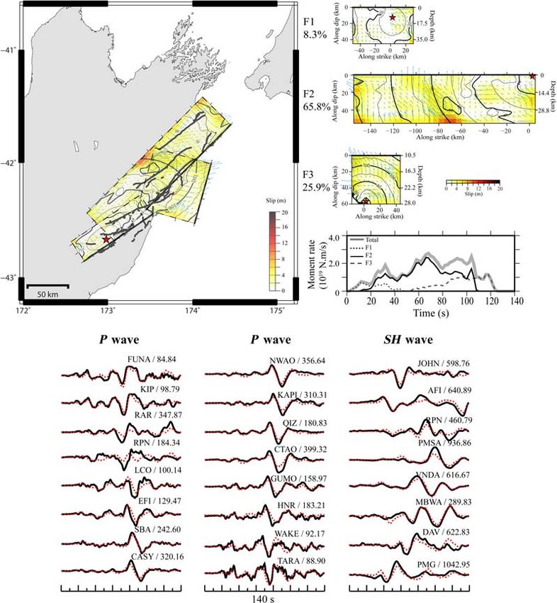
4                                                                                                        Y.-Y. Wen, K.-F. Ma, and B. Fry

Figure 3.     Slip model from the teleseismic waveform inversion and comparison of the observed (solid line) and the synthetic (dashed line)
waveforms. Stars show the initiation locations on each segment, and arrows and contours indicate the slip vectors and rupture time, re-
spectively. The station name and peak value of the record in micrometers are shown above the waveforms. The number below each segment
indicates the percentage of seismic moment released. The color version of this figure is available only in the electronic edition.

rate GPS data record this dominant displacement pulse on                only GPS offsets, and (3) fitting both teleseismic and GPS
stations located in the northern half of the rupture (Kaiser            data. For the inversions fitting only teleseismic data, the
et al., 2017). On the other hand, the location of the main              optimal model with a misfit of ε  0:417 indicates that
moment-rate burst backprojected from Rayleigh-wave data                 the 2016 Kaikoura earthquake initially ruptured with a veloc-
(Duputel and Rivera, 2017) is similar with the model derived            ity of 2:0 km=s in segment F1, followed by 1:75 km=s in
from geodetic data (Hamling et al., 2017) and is located near           segment F2, and propagated to segment F3 with a very slow
42° S. Therefore, we limit the rupture front propagation                velocity of 1:0 km=s. This slow rupture speed is somewhat
through this region to between 60 and 80 s after the initiation,        compatible with backprojection analysis of Hollingsworth
and we also apply a seismic moment constraint, based on the             et al. (2017), which suggests rupture velocities were in
Global CMT solution, in the inversion.                                  1:5–2:5 km=s range. We apply a multiple-time-window
                                                                        modeling scheme with the derived optimum rupture velocity
                             Results                                    variation using eight 4-s duration triangles lagged by 2 s each,
     To compare the information about the source process                for maximum subfault rupture durations of 18 s. The slip model
derived from various data, we carry out three inversion pro-            with ε  0:340 and comparison of modeled and observed
cedures: (1) fitting only teleseismic waveforms, (2) fitting            waveforms are shown in Figure 3. The total seismic moment

                                                          BSSA Early Edition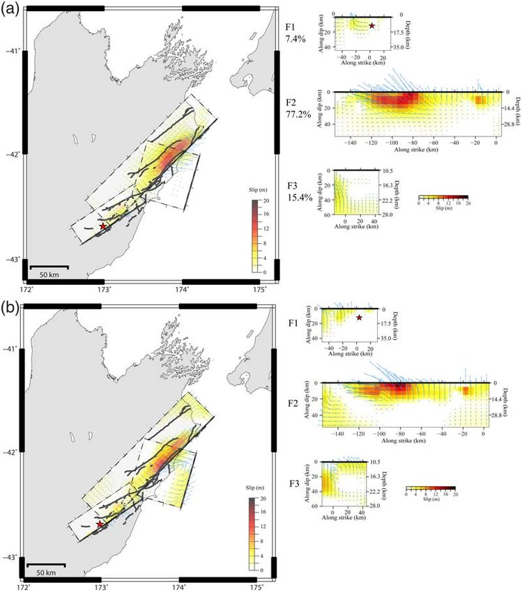
Multiple-Fault, Slow Rupture of the 2016 Kaikoura Earthquake                                                                             5

Figure 4. Slip model from (a) GPS offset inversion and (b) the GPS residual from teleseismic waveform inversion model. The star shows
the epicenter location. The number below each segment indicates the percentage of seismic moment released. The color version of this figure
is available only in the electronic edition.

is 8:90 × 1020 N · m (M w 7.90). The model exhibits a very              shallow part of segment F2, corresponding to the main en-
weak initiation with relatively little slip in segment F1, and          ergy released on the Jordan thrust and Kekerengu faults. Seg-
one obvious asperity on segment F2 that ruptured with large             ment F3 ruptured with large amounts of deep reverse slip,
amounts of slip at deeper depths, and a generally smoother slip         which is consistent with the location and faulting mechanism
distribution on the subduction interface F3. These features             revealed by Duputel and Rivera (2017). The total seismic
coincide with two large subevents located near 42° S that               moment is 8:03 × 1020 N · m (M w 7.87).
released energy about 60–80 s after the origin time in the in-               The joint inversion best fits the data with relatively slow
version results of Duputel and Rivera (2017). The northern              rupture velocities for F2 and F3. The optimal model (misfit
end of F2 displays significant strike-slip motion in the shallow        of ε  0:554) suggests that the Kaikoura earthquake initially
part that may reflect the rupture of the Needles fault.                 ruptured with a velocity of 2:25 km=s in segment F1, slowed
      The inverted model fitting only GPS data (misfit of               down to 1:50 km=s in segment F2, and then rupture propa-
ε  0:020) is shown in Figure 4a. This model is similar to              gated across F3 at 1:0 km=s. The significantly slow velocity
the model derived from geodetic data (Hamling et al., 2017).            in segment F2 is comparable with the average rupture speed
The rupture sequence began with relatively minor slip-on                of 1:4 km=s estimated from backprojection imaging by
segment F1, followed by rupture of the main asperity on the             Zhang et al. (2017) as well as the average rupture velocity
                                                         BSSA Early Edition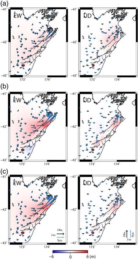
6                                                                                                        Y.-Y. Wen, K.-F. Ma, and B. Fry

Figure 5. Slip model from joint inversion and comparison of the observed (solid line) and the synthetic (dashed line) waveforms. Stars
show the initiation locations on each segment, and arrows and contours indicate the slip vectors and rupture time, respectively. The station
name and peak value of the record in micrometers are shown above the waveforms. The number below each segment indicates the percentage
of seismic moment released. The color version of this figure is available only in the electronic edition.

of 1:5 km=s derived from the joint inversion by Wang et al.             Zhang et al., 2017). However, because of the limited resolu-
(2018). Figure 5 shows the final slip model and waveform                tion of teleseismic data and the simplified fault geometries,
fitting, with a misfit of ε  0:457, after applying multiple-           models derived purely from teleseismic data can provide
time-window modeling scheme. This joint inversion model                 the primary source time process and slip pattern, especially at
also reveals a weak initiation with little slip in segment F1,          greater depths, but lack the resolution to reveal slip patterns at
however, there is a significant main asperity in segment F2             shallow depths. On the other hand, the geodetic data can better
and a minor asperity in the deeper part of segment F3. The              constrain the slip pattern at shallow depths, yet are relatively
total seismic moment is 9:91 × 1020 N · m (M w 7.93).                   insensitive to deeper kinematics and contain no timing or rup-
                                                                        ture velocity information. Both our teleseismic-only model
                                                                        and those derived from seismic data (Hollingsworth et al.,
                Discussion and Conclusions
                                                                        2017; Zhang et al., 2017) reveal large amounts of deep slip.
     All of the optimal models from both the joint inversion            Although the locations of dominant energy released in
and the teleseismic-only inversion reveal slow rupture proc-            segments F2 and F3 (Fig. 3) are consistent with the main
esses during the 2016 Kaikoura earthquake. This is consistent           moment-rate burst backprojected from the Rayleigh-wave
with the result of previous studies (Duputel and Rivera, 2017;          data (Duputel and Rivera, 2017), the synthetic surface dis-
Holden et al., 2017; Kaiser et al., 2017; Wang et al., 2018;            placements do not fit the observations. Figure 6a shows the
                                                          BSSA Early Edition
Multiple-Fault, Slow Rupture of the 2016 Kaikoura Earthquake 7
inversion model (Fig. 5). The synthetic coseismic displace-
ments still exhibit good fits to both amplitude and orientation.
To resolve the possible slip distribution at shallower depths,
we also calculate the difference between the synthetic GPS
from the teleseismic slip model and the observed GPS offsets.
Then, we use this difference to invert a slip model (Fig. 4b),
which is more sensitive to shallow deformation. Differences in
the slip patterns of Figure 4b to 4a (GPS alone) and Figure 3
(teleseismic data alone) suggest that the geodetic data better
constrain both slip within depths of 0–20 km and the northern
edge of F3, whereas teleseismic data well extract slip at deeper
depth and are sensitive to the northern offshore rupture of F2.
These general features are consistent with the results shown in
Figure 5 of the spatial slip distribution from joint inversion and
suggest the reliability of this joint analysis.
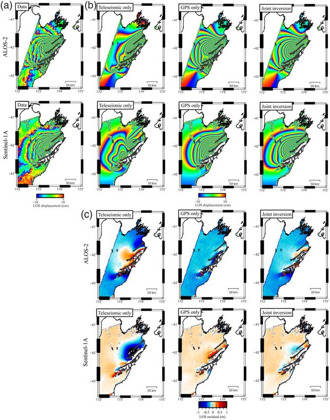
We further conducted a forward simulation of synthetic
aperture radar (SAR) interferograms (Fig. 7), which were
not incorporated in the inversion process. For calculating
the displacements of radar line of sight (LOS), average look-
ing vectors (east, north, and up) are used: (−0:6761, 0.2205,
and −0:7015) for the descending ALOS-2 interferogram and
(0.5986, 0.1923, and −0:7748) for the ascending Sentinel-1A
interferogram (data and parameters were provided by Ian
J. Hamling). Although our teleseismic waveform inversion
model is roughly compatible with results from other seismo-
logical studies (Hollingsworth et al., 2017; Zhang et al.,
2017), the slip vectors at shallow depths are much smaller than
those of the model derived from geodetic data (Hamling et al.,
2017), especially near the Kekerengu fault. Therefore, as
shown in Figure 7, both the synthetic descending and ascend-
ing interferograms derived from the teleseismic waveform in-
version model (Fig. 3) fail to reproduce the density of fringes
in the SAR observations, which indicates insufficient ground
displacements. This points out the difficulty in resolving slip
portioning, especially for the shallow slip, using teleseismic
waveforms alone. Conversely, both the synthetic descending
and ascending interferograms derived from the GPS offset in-
version (Fig. 4a) and joint inversion models (Fig. 5) match
Figure 6. Modeled horizontal (EW) and vertical (UD) displace- fringe patterns contained in the observations quite well, except
ments from (a) teleseismic waveform inversion, (b) GPS offset in- for the near-fault area, as shown in Figure 7. Interestingly,
version, and (c) joint inversion results. Solid and open arrows show when comparing the LOS residual of different models, the
the observed and synthetic displacements at GPS stations. The star joint inversion model better fits the measured LOS in the
shows the epicenter location. The color version of this figure is western off-fault region. This again suggests the need for slip
available only in the electronic edition.
at deeper depths contributed from the teleseismic data, and the
geodetic data providing further constrain on the most near-
synthetic static ground displacements derived from the tele- fault region.
seismic waveform inversion model (Fig. 3). Although the Several studies have shown the complex fault segmen-
orientations of synthetic displacement are mostly consistent tation and large rupture speed variation for this 2016
with the GPS observations, the synthetic displacement under- Kaikoura earthquake (Hamling et al., 2017; Holden et al.,
estimates the measured displacement. Figure 6b shows the 2017; Wang et al., 2018). However, the simplified fault
synthetic static ground displacement derived from the GPS geometries with fixed rupture velocity for each segment limit
offset inversion model (Fig. 4a). With the exception of some the exploration of the faulting process. The moment rate
near-fault stations, the synthetic coseismic displacements well functions in Figures 3 and 5 show a longer duration than
reproduced the amplitude and orientation of the observations other studies. This could be expected and is mainly due
for both amplitude and orientation. Figure 6c shows the to the slow and fixed rupture velocity for the long segment
synthetic static ground displacements derived from the joint F2. Even though, our joint inversion model can explain both
BSSA Early Edition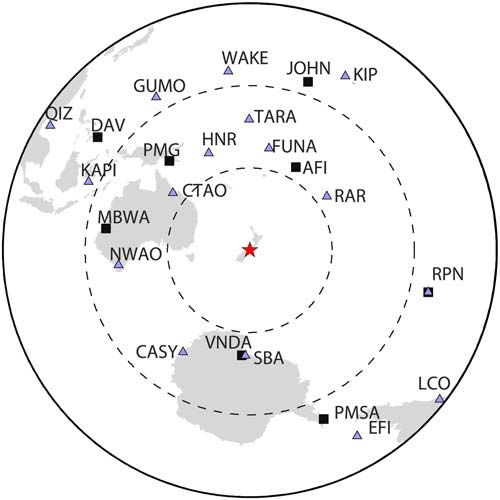
8                                                                                                           Y.-Y. Wen, K.-F. Ma, and B. Fry

Figure 7. (a) Observed, (b) modeled, and (c) residuals of ALOS-2 and Sentinel-1A interferograms from teleseismic waveform inversion,
GPS offset inversion, and joint inversion results, respectively. The star shows the epicenter location. LOS, line of sight. The color version of
this figure is available only in the electronic edition.

the far-field (teleseismic data) and near-field (GPS and In-              show that the 2016 Kaikoura earthquake released seismic
SAR data) observations and reveal the main rupture proper-                moment on the subduction plate interface during the faulting
ties of the 2016 Kaikoura earthquake.                                     (e.g., Bai et al., 2017; Duputel and Rivera, 2017; Hamling
     By integrating the rupture information extracted from the            et al., 2017; Wang et al., 2018), whereas some studies model
teleseismic data and GPS data, our joint inversion model sug-             the mainshock rupture process with shallower strike-slip and
gests that the 2016 Kaikoura earthquake ruptured northeast-               thrust faults only (Cesca et al., 2017; Holden et al., 2017;
ward with a weak initiation, significant thrust motion in the             Zhang et al., 2017). In our three models (Figs. 3–5), the
northern part of the Hope and/or Humps and Hundalee faults,               slip-on segment F3 released 15%–25% of the total seismic
large oblique motion along the Kekerengu fault, and some                  moment, and the amounts are much smaller than those of seg-
strike-slip displacement on the Needles fault. Several studies            ment F2 (65%–80% of the total seismic moment). Figure 8
                                                            BSSA Early Edition
Multiple-Fault, Slow Rupture of the 2016 Kaikoura Earthquake 9
ment F1 contains relatively large HF radia-
tion. The region with a large asperity with
slow rupture velocity (1:5 km=s) in seg-
ment F2 lacks HF energy radiation, whereas
an HF source was detected near to the rup-
ture front of main asperity of segment F2,
mostly south of −42°. The variation of rup-
ture speed and the compensation of the en-
ergy release in HF and LP sources describe
complex rupture dynamics during the fault-
ing of the 2016 Kaikoura earthquake. Dur-
ing the faulting process, the rupture velocity
is strongly related to the strength and stress
state of the fault, fault geometry, and the
fracture energy (Rosakis, 2002; Kanamori
and Rivera, 2006). Complex multifault rup-
ture, such as the 2016 Kaikoura earthquake,
requires time for stress transfer from the ad-
jacent faults to reach the critical status of
rupture and thus slows down the propaga-
tion speed. Numerous slow-slip events have
been identified in Hikurangi subduction
margin (Wallace and Beavan, 2010), and
the 1947 Offshore Poverty Bay tsunami
earthquake even ruptured with a very slow
speed of 150–300 m=s (Bell et al., 2014).
This suggests that the slow rupture velocity
during the 2016 Kaikoura earthquake is rea-
sonable and perhaps a fundamental character-
istic of the southern Hikurangi megathrust.
Italsopresentsamechanismtogeneratemuch
of the LP long-duration ground motions
observed (Bradley et al., 2017; Kaiser
et al., 2017) at local and regional distances.
Our results, coupled with evidence of slow
Figure 8. Comparison of the observed (solid line) and the synthetic (dashed line) rupture elsewhere along the Hikurangi
waveforms contributed from segment F3 for models of (a) teleseismic waveform inver-
margin, suggest that slow rupture and the
sion and (b) joint inversion, respectively. The station name and peak value of the record
in micrometers are shown above the waveforms. The color version of this figure is avail- resulting increase in tsunami potential and
able only in the electronic edition. LP ground motion should be considered in
future hazard studies in the region.
shows the contribution of segment F3 to the seismic records Data and Resources
for teleseismic waveform inversion model and joint inversion
model, and it mainly explains the minor pulses later than 90 s, All data used in this article came from published
which are close to the end of faulting (Bai et al., 2017; Cesca sources listed in the References section, and all figures
et al., 2017; Duputel and Rivera, 2017; Zhang et al., 2017; were generated using the Generic Mapping Tools v. 4.5.8
Wang et al., 2018). Thus, similar to the conclusion of Holden (www.soest.hawaii.edu/gmt/, last accessed December 2017;
et al. (2017), most of the faulting process of the 2016 Kai- Wessel and Smith, 1998). Global Centroid Moment Tensor
koura mainshock can be explained by the movement on (CMT) solution is available at https://earthquake.usgs.gov
the crustal faults. However, the contribution from the subduc- (last accessed December 2017).
tion interface is less, but required, and this is similar to the
result of Wang et al. (2018). In comparison with the high-fre- Acknowledgments
quency (HF) sources imaged from backprojection analysis of
The authors thank editor Ian J. Hamling and two anonymous reviewers
Hollingsworth et al. (2017) and Zhang et al. (2017), our joint for their helpful comments. This research was supported by the Taiwan
inversion revealed the energy release of LP sources. The weak Earthquake Center (TEC) and funded by the Ministry of Science and Tech-
initiation with the highest rupture speed (2:25 km=s) in seg- nology, Taiwan (MOST 106-2116-M-194-008). The TEC Contribution
BSSA Early Edition10 Y.-Y. Wen, K.-F. Ma, and B. Fry
Number for this article is 00142. The contribution of B. F. to this work was Great Peruvian earthquakes of 23 June 2001 and 15 August 2007, Bull.
supported by a grant from the Royal Society of New Zealand. Seismol. Soc. Am. 100, 969–994, doi: 10.1785/0120090274.
Lee, S. J., W. T. Liang, L. Mozziconacci, Y. J. Hsu, W. G. Huang, and B. S.
References Huang (2013). Source complexity of the 4 March 2010 Jiashian,
Taiwan earthquake determined by joint inversion of teleseismic and
Bai, Y., T. Lay, K. F. Cheung, and L. Ye (2017). Two regions of seafloor near field data, J. Asian Earth Sci. 64, 14–26, doi: 10.1016/j.
deformation generated the tsunami for the 13 November 2016, jseaes.2012.11.018.
Kaikoura, New Zealand earthquake, Geophys. Res. Lett. 44, 6597– Litchfield, N. J., A. Benson, A. Bischoff, A. Hatem, A. Barrier, A. Nicol, A.
6606, doi: 10.1002/2017GL073717. Wandres, B. Lukovic, B. Hall, C. Gasston, et al. (2016). 14th November
Bassin, C., G. Laske, and G. Masters (2000). The current limits of resolution for 2016 M 7.8 Kaikoura earthquake. Preliminary surface fault displace-
surface wave tomography in North America, Eos Trans AGU 81, F897. ment measurements, Version 2, GNS Science doi: 10.21420/G2J01F.
Bell, R., C. Holden, W. Power, X. Wang, and G. Downes (2014). Hikurangi Litchfield, N. J., R. Van Dissen, R. Sutherland, P. M. Barnes, S. C. Cox, R.
margin tsunami earthquake generated by slow seismic rupture over a Norris, R. J. Beavan, R. Langridge, P. Villamor, K. Berryman, et al.
subducted seamount, Earth Planet. Sci. Lett. 397, 1–9, doi: 10.1016/j. (2014). A model of active faulting in New Zealand, New Zeal. J. Geol.
epsl.2014.04.005. Geophys. 57, 32–56.
Bradley, B. A., H. N. T. Razafindrakoto, and V. Polak (2017). Ground- Litchfield, N. J., P. Villamor, R. J. Van Dissen, A. Nicol, P. M. Barnes, D. J.
motion observations from the 14 November 2016 Mw 7.8 Kaikoura, A. Barrell, J. Pettinga, R. M. Langridge, T. A. Little, J. Mountjoy, et al.
New Zealand earthquake and insights from broadband simulations, (2017). Surface fault ruptures from the M w 7.8 2016 Kaikōura earth-
Seismol. Res. Lett. 88, no. 3, 1–17, doi: 10.1785/0220160225. quake and insights into factors controlling multi-fault ruptures, Bull.
Cesca, S., Y. Zhang, V. Mouslopoulou, R. Wang, J. Saul, M. Savage, S. Seismol. Soc. Am. this issue.
Heimann, S.-K. Kufner, O. Oncken, and T. Dahma (2017). Complex Rosakis, A. J. (2002). Intersonic shear cracks and fault ruptures, Adv. Phys.
rupture process of the Mw 7.8, 2016, Kaikoura earthquake, 51, 1189–1257.
New Zealand, and its aftershock sequence, Earth Planet. Sci. Lett. Wallace, L., and J. Beavan (2010). Diverse slow slip behavior at the
478, 110–120, doi: 10.1016/j.epsl.2017.08.024. Hikurangi subduction margin, New Zealand, J. Geophys. Res. 115,
Duputel, Z., and L. Rivera (2017). Long-period analysis of the 2016 no. B12402, doi: 10.1029/2010JB007717.
Kaikoura earthquake, Phys. Earth Planet. In. 265, 62–66, doi: Wang, T., S. Wei, X. Shi, Q. Qiu, L. Li, D. Peng, R. J. Weldon, and S. Barbot
10.1016/j.pepi.2017.02.004. (2018). The 2016 Kaikōura earthquake: Simultaneous rupture of the
Eberhart-Phillips, D., and S. Bannister (2010). 3-D imaging of Marlborough, subduction interface and overlying faults, Earth Planet. Sci. Lett.
New Zealand, subducted plate and strike-slip fault systems, Geophys. 482, 44–51, doi: 10.1016/j.epsl.2017.10.056.
J. Int. 182, no. 1, 73–96, doi: 10.1111/j.1365-246X.2010.04621.x. Wen, Y.-Y., and K.-F. Ma (2010). Fault geometry and distribution of asper-
Fry, B., D. Eberhart-Phillips, and F. J. Davey (2014). Mantle accommodation ities of the 1997 Manyi, China (M w 7:5), earthquake: Integrated
of lithospheric shortening as seen by combined surface wave and tele- analysis from seismological and InSAR data, Geophys. Res. Lett.
seismic imaging in the South Island, New Zealand, Geophys. J. Int. 37, L05303, doi: 10.1029/2009GL041976.
199, no. 1, 499–513, doi: 10.1093/gji/ggu271. Wen, Y.-Y., K.-F. Ma, and D. D. Oglesby (2012). Variations in rupture speed,
Hamling, I. J., S. Hreinsdóttir, K. Clark, J. Elliott, C. Liang, E. Fielding, N. slip amplitude, and slip direction during the 2008 Mw 7.9 Wenchuan
Litchfield, P. Villamor, L. Wallace, T. J. Wright, et al. (2017). Complex earthquake, Geophys. J. Int. 190, 379–390, doi: 10.1111/j.1365-
multifault rupture during the 2016 Mw 7.8 Kaikōura earthquake, 246X.2012.05476.x.
New Zealand, Science doi: 10.1126/science.aam7194. Wessel, P., and W. H. F. Smith (1998). New, improved version of generic
Hartzell, S. H., and T. H. Heaton (1983). Inversion of strong ground motion and mapping tools released, Eos Trans. AGU 79, 579.
teleseismic waveform data for the fault rupture historyofthe 1979Imperial Zhang, H., K. D. Koper, K. Pankow, and Z. Ge (2017). Imaging the 2016
Valley, California earthquake, Bull. Seismol. Soc. Am. 73, 1553–1583. M w 7.8 Kaikoura, New Zealand, earthquake with teleseismic P waves:
Holden, C., Y. Kaneko, E. D'Anastasio, R. Benites, B. Fry, and I. J. Hamling A cascading rupture across multiple faults, Geophys. Res. Lett. 44,
(2017). The 2016 Kaikōura earthquake revealed by kinematic source 4790–4798, doi: 10.1002/2017GL073461.
inversion and seismic wavefield simulations: Slow rupture propagation
on a geometrically complex crustal fault network, Geophys. Res. Lett.
doi: 10.1002/2017GL075301. Department of Earth and Environmental Sciences
Hollingsworth, J., L. Ye, and J.-P. Avouac (2017). Dynamically triggered slip National Chung-Cheng University
on a splay fault in the Mw 7.8, 2016 Kaikoura (New Zealand) earthquake, Chia-Yi County 62102, Taiwan
Geophys. Res. Lett. 44, 3517–3525, doi: 10.1002/2016GL072228. yiyingwen@ccu.edu.tw
Ji, C., D. J. Wald, and D. V. Helmberger (2002). Source description of the (Y.-Y.W.)
1999 Hector Mine earthquake; Part I: Wavelet domain inversion theory
and resolution analysis, Bull. Seismol. Soc. Am. 92, 1207–1226.
Kaiser, A., N. Balfour, B. Fry, C. Holden, N. Litchfield, M. Gerstenberger, Earthquake Disaster & Risk Evaluation and Management (E-DREaM)
E. D'Anastasio, N. Horspool, G. McVerry, J. Ristau, et al. (2017). The Center
2016 Kaikōura, New Zealand, earthquake: Preliminary seismological re- Department of Earth Sciences
port, Seismol. Res. Lett. 88, no. 3, 727–739, doi: 10.1785/0220170018. National Central University
Kanamori, H., and L. Rivera (2006). Energy partitioning during an earth- Taoyuan City 32001, Taiwan
quake, in Earthquakes: Radiated Energy and the Physics of Faulting, (K.-F.M.)
R. Abercrombie, A. McGarr, G. Di Toro, and H. Kanamori (Editors),
Geophysical Monograph Series, Vol. 170, AGU Chapman Volume,
AGU, Washington, D. C., 3–13, doi: 10.1029/170GM03. GNS Science
Langston, C. L., and D. V. Helmberger (1975). A procedure for modeling Avalon
shadow dislocation source, Geophys. J. Roy. Astron. Soc. 42, 117–130. Lower Hutt 5040, New Zealand
Lawson, C. L., and R. J. Hanson (1974). Solving Least Squares Problems, (B.F.)
Prentice Hall, Englewood Cliffs, New Jersey.
Lay, T., C. J. Ammon, A. R. Hutko, and H. Kanamori (2010). Effects of Manuscript received 29 September 2017;
kinematic constraints on teleseismic finite-source rupture inversions: Published Online 17 April 2018
BSSA Early EditionYou can also read