Surface Type Classification for Autonomous Robot Indoor Navigation
←
→
Page content transcription
If your browser does not render page correctly, please read the page content below
Surface Type Classification for Autonomous Robot
                Indoor Navigation
  Francesco Lomio∗ , Erjon Skenderi, Damoon Mohamadi, Jussi Collin, Reza Ghabcheloo and Heikki Huttunen
                                                             Tampere University, Finland

   Abstract—In this work we describe the preparation of a
time series dataset of inertial measurements for determining the
surface type under a wheeled robot. The data consists of over
7600 labeled time series samples, with the corresponding surface
type annotation. This data was used in two public competitions
with over 1500 participant in total. Additionally, we describe the
performance of state-of-art deep learning models for time series
classification, as well as propose a baseline model based on an
ensemble of machine learning methods. The baseline achieves an
accuracy of over 68% with our nine-category dataset.
   Index Terms—Floor Surface, Classification, Deep Learning,
Autonomous Machine, Inertial Measurement Unit

                           I. I NTRODUCTION
   Indoor and outdoor navigation has become an important
                                                                           Fig. 1. Variation of one of the measures recorded by the IMU for two classes.
concept for autonomous machines such as mobile robots and
intelligent work machines. Most navigation techniques rely
on external sources, such as geolocation based on Global                   robot with the terrain (both indoor and outdoor) for classifying
Positioning System (GPS), Global Navigation Satellite System               the surface type.
(GNSS), Bluetooth Low Energy (BLE) or WIFI. However,                          We describe a procedure of data collection from nine
the navigation accuracy could be improved from novel data                  indoor surface types collected using only an IMU sensor
sources, that are not directly connected with the location, but            positioned on an industrial trolley with silent wheels. Each
serve as a proxy target to be used for data fusion.                        measurement sequence is linked with the actual surface. To
   One such proxy measurement of location is the surface type              the best of our knowledge, the dataset is unique both in its
underneath the autonomous vehicle. For example, the map                    extent, as well as its scope. The data was used in two public
may contain data of all surface types, and with an inertial                machine learning competitions: first as a mandatory part of a
measurement unit (IMU), once the measurement system de-                    university advanced machine learning course1 ; and secondly
tects a transition in the surface type, this fixes the location in         as a public competition for all participants of a worldwide
the map, making the navigation data more reliable.                         CareerCon2 event organized by Kaggle—a company whose
   To this aim, this work describes a new dataset generated                platform is used for organizing large scale machine learning
using an inertial measurement unit, whose variation can be                 competitions. In total, over 1,500 people have participated in
used for surface type classification (Figure 1), along with a              those competitions.
machine learning based approach for surface type classifica-                  Beside introducing the dataset, in this work we also illus-
tion.                                                                      trate the results obtained by two state-of-art deep learning
   Other work have shown the possibility of using this type                models for time series classification, tested on our proposed
of sensors for the surface recognition, using data related to              dataset, as well as a baseline model based on an ensemble of
outdoor surfaces [1]. In [2], the authors used the Z-axis                  classical machine learning tool and deep learning.
of the accelerometer of an IMU unit as input to classify                      Thus, to summarize, the main contributions of the paper are
the surface type for different velocity, but this was done                 the following: (1) we release the most comprehensive dataset
only for outdoor data. In [3], the authors used sensors from               for indoor surface categorization to date and (2) we propose a
legged walking robots to classify indoor surface. Other studies            baseline, which is fused from recent time series classification
used a combination of multiple sensors and cameras [4].                    models and community methods that have proven successful
In [5], the authors studied a method for a robot to learn to               in two competitions using our data. Finally, (3) the dataset is
classify outdoor surface from vibration and traction sensors               made publicly available in its entirety, which we hope will
and use these information to learn to recognize the type of                spread to public use within the machine learning community
terrain ahead from an inbuilt camera. Other approaches for                 as a standard benchmark dataset3 .
the surface recognition include the use of audio data: in [6]
                                                                             1   www.kaggle.com/c/robotsurface
the authors used the audio feedback from the interaction of the              2   www.kaggle.com/c/career-con-2019
  ∗ Corresponding   author; email: francesco.lomio@tuni.fi                   3   www.zenodo.org/record/2653918#.XMgP2MRS-Uk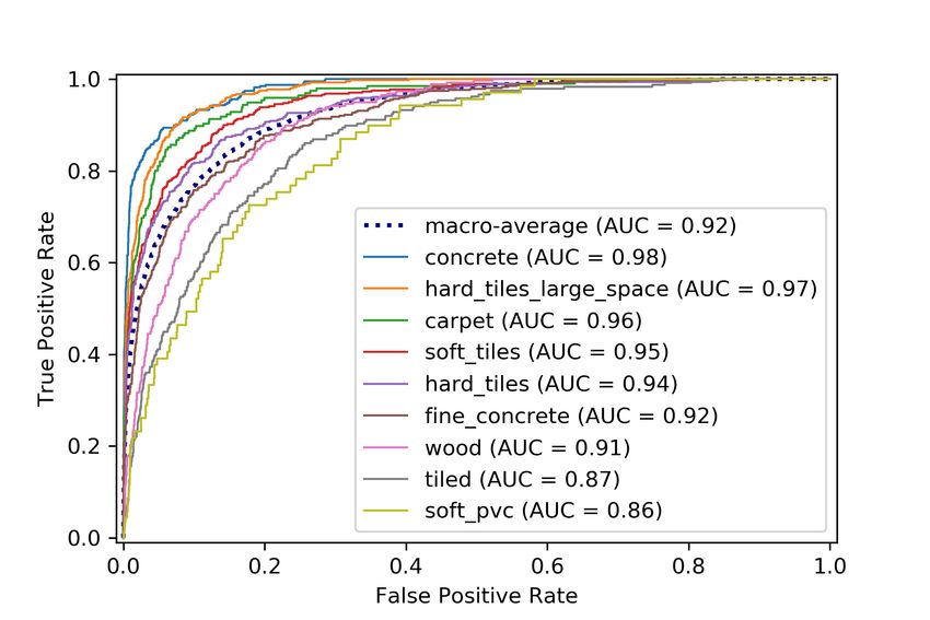
Fig. 2. Sample distribution by class.
In the remainder of this paper, we describe the data collec- window of consecutive data point in order to obtain segments
tion procedure in Section II together with the characteristics of length 128 points. After this process, our dataset includes
of the data and a discussion of the preparation to a suitable 7626 segments.
form for a large scale competition. Next, Section III discusses The sample distribution by class is shown in Figure 2.
the method used to test the data, specifically some state-of- From this, it can be seen that some of the classes are under-
art methods for time series classification. We also describe a represented. In order to avoid that during the testing of the
baseline model, consisting of an ensemble of machine learning models some of the class were totally absent from the test set,
method and deep learning for the surface type classification. we made sure during the cross validation process to have all
The results of the models used are discussed in Section IV. Fi- classes represented in both the train and the test set.
nally, Section V summarizes the results and discusses further Moreover, we divided the data into groups to be used for
work on this domain. the cross validation. A group is a collection of subsequent
128-sample long segments and in total we have 80 groups.
II. DATA COLLECTION AND PREPARATION We noticed that a random train-test split would lead an overly
A. Data collection optimistic accuracy estimate as neighboring samples would
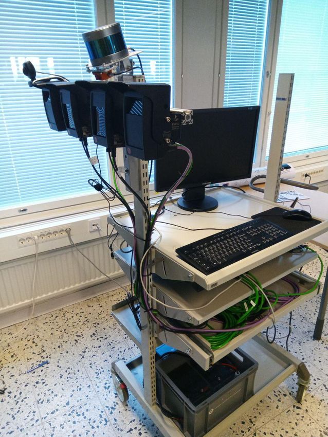
The data was collected using an industrial trolley with silent be in train and test sets. On the other hand, a systematic
wheels shown in the Figure 3. The trolley has no motors and it split by time (e.g., first third of each sequence for training,
was pushed across the corridors and offices. The machine was second for validation and third for testing) would probably
equipped with an Inertial Measurement Units (IMU sensor). give pessimistic and misleading accuracy estimates as the
The IMU sensor used is an XSENS MTi-300. The sensor data state (e.g., direction) could have changed radically. Thus, our
collected includes accelerometer data, gyroscope data (angular compromise is to group adjacent segments together, and split
rate) and internally estimated orientation. Specifically: the data such that each group belongs fully into one of the
three folds, which makes the classification process fair and
– Orientation: 4 attitude quaternion channels, 3 for vector
less biased.
part and one for scalar part;
– Angular rate: 3 channels, corresponding to the 3 orthog- C. Setting up a machine learning competition
onal IMU coordinate axes X, Y, and Z; The data was used in two public machine learning competi-
– Acceleration: 3 channels, specific force corresponding to tion, both hosted on the Kaggle platform. The platform is free
3 orthogonal IMU coordinate axes X, Y, and Z. of charge for educational use, and these InClass competitions
While angular velocity and linear acceleration are given have shown their importance for exposing machine learning
in the IMU body coordinates X, Y, and Z, the orientation students to practical machine learning challenges [8]. How-
is presented as a quaternion, a mathematical notation used ever, setting up the competition requires careful design as any
to represent orientations and rotations in a 3D space [7]. coursework in order to encourage exploration and learning.
The setup was driven through a total of 9 different surface The platform requires the data to be split in train, validation,
types: hard tiles with large space, hard tiles, soft tiles, fine and test folds. The validation and test set are used respectively
concrete, concrete, soft polyvinyl chloride (PVC), tiles, wood, to score the submission of the participants in the public and
and carpet. the private leaderboards. As the name suggests, the public
Each data point includes the measures described above of leaderboard is visible to everyone for the whole duration of
orientation, velocity and acceleration, resulting in a feature the competition and can be used for assessing the performance
vector of length 10 for each point. In total almost a million of one’s own model. The private leaderboard is only visible
data points were collected. once the competition ends and it is the basis for deciding the
final scoring of the participant’s model.
B. Data preparation It is not uncommon for the results to vary widely between
In order to preserve the characteristics of the time series the public and the private leaderboards, specifically if the data
corresponding to different surface types, we grouped a fixed in the validation set is significantly different from the one inthe test set. From an educational point of view, this can cause the second model is a Fully Convolutional Network (FCN),
disappointment and discouragement for the young students while the third is a Residual Network (ResNet). These last
participating in the competition, undermining the purpose of two approaches are adopted from [12], where the authors
the course. To avoid this, we split the data training a Gaussian found their performance superior to a number of other tested
Mixture Model (GMM) [9] for each of the set and measuring methods. Specifically, Fawaz et al. showed in their work that
the symmetric Kullback-Leiber (KL) divergence [10] [11], in the FCN and the ResNet were the top performing methods
order for it to be minimized between the validation and the for multivariate time series classification. This results were
test set. Specifically, we created 3 sets (train, validation and obtained testing 9 different classifiers on 12 multivariate time
test) by random shuffling and dividing the segments, such that series datasets.
50% of the data was used for the training set, and 25% each in Besides studying each method singularly, we also study the
the validation and the test sets. We trained a GMM for each fusion of the three methods by combining their predictions
set and we measured the distance between them using the together in various ways. This method is a derivation of the
symmetric KL divergence. We did this iteratively for 1000 winning model from our first, university level course, Kaggle
different splits, and chose the one with the minimum KL competition. The winning team in fact used a combination
divergence between the validation and test set. of XGBoost and 1-dimensional convolutional networks to
The orientation is estimated internally by the IMU by fusing classify the surface type.
accelerometer data, gyro data and optionally magnetometer All the tests in our study have been conducted using only
data. In this process the gyro data is integrated over time, six of the ten channels available in the dataset. In fact,
and furthermore, the integration is non-commutative [7]. This we excluded the orientation channel because of the scarce
means that segments can be identified with potentially high correlation that it has to the surface type, as we discovered
confidence by linking an end of one segment quaternion to a from the results and discussion of the two public competition.
start of another segment quaternion. This is a potential source We still decided to include it in the dataset as it can be useful
of leak for competitions where continuous data is scrambled. for future works.
Furthermore, in practical applications the orientation is inde-
pendent of surface type and orientation-based features can lead A. Manually engineered features
to a model that over-fits the training data. On the other hand, The first method used is based on a XGBoost model [13],
quaternions can be used to rotate the inertial measurements to a state-of-the-art, optimized, implementation of the Gradient
locally level frame and this leads to improved sensitivity in Boosting algorithm. It allows faster computation and paral-
surface detection. This leak was in fact recognized by some of lelization compared to normal boosting algorithm. For this
the competitors, resulting in an unrealistically high accuracy, reason it can yield better performance compared to the latter,
as we will discuss in the experimental section. and can be more easily scaled for the use with high dimen-
sional data. In our case, we trained a tree based XGBoost
model, with 1000 estimators and a learning rate of 10−2 .
This model uses the following human-designed basic fea-
tures: We compute the mean, the standard deviation, and the
fast fourier transform (FFT) of each of the six measurement
channels, and used these three features for the training of
the model. Specifically the FFT was included for its ability
to simplify complex repetitive signals, highlighting their key
components.
B. Fully Convolutional Neural Network
The second method used, is a fully convolutional neural
network (FCN) [14]. This convolutional network does not
present any pooling layer (hence the name), therefore the
dimension of the time series remains the same through all the
convolution. Moreover, after the convolutions, the features are
Fig. 3. Data collection set-up. The IMU sensor is the orange box positioned passed to a global average pooling (GAP) layer [15] instead
under the LIDAR of the more traditional fully connected layer. The GAP layer
allows the features maps of the convolutional layers to be
III. M ETHODS recognised as category confidence map. Moreover, it reduces
We study three alternative methods for classifying the floor the number of parameters to train in the network, making it
surface type. The first approach is a traditional combination more lightweight, and reducing the risk of overfitting, when
of manual feature engineering coupled with a state-of-the- compared to the fully convolutional layer.
art classifier, with manually engineered features specifically The FCN used in this work, adopted from [12], consists
tailored for this task. The second and third approach use a of 3 convolutional blocks, each composed by a 1-dimensional
convolutional neural network, whose convolutional pipeline convolution followed by a batch normalization layer [16] and
learns the feature engineering from the data. More specifically, a rectified linear unit (ReLU) [17] activation function. Theoutput of the last convolutional block are fed to the GAP TABLE I
layer, to which a traditional softmax is fully connected for E VALUATION SCORE FOR THE MODELS USED .
the time series classification. Accuracy score AUC score
XGBoost 59.54% ± 5.57% 89.59% ± 1.51%
C. Residual Network FCN 62.69% ± 6.74% 90.45% ± 2.20%
The last method used is a residual network (ResNet) [14], ResNet 64.95% ± 3.39% 92.33% ± 1.16%
XGB + FCN 64.87% ± 6.14% 91.26% ± 1.77%
composed by 11 layers of which 9 are convolutional. The XGB + ResNet 65.76% ± 3.97% 91.40% ± 1.46%
main difference with the FCN described before is the presence FCN + ResNet 67.57% ± 4.34% 92.30% ± 1.62%
of shortcut connection between the convolutional layers. This XGB + FCN + ResNet 68.21% ± 5.12% 91.98% ± 1.65%
connections allow the network to learn the residual [18]. This
allow the network to be more easily training, as the gradient
flows directly through the connections. Moreover, the residual between the train and the test set, making the classification
connection allow to reduce the vanishing gradient effect. task biased. Using an iterated cross validation over groups of
In this work we used the ResNet shown in [12]. It consists samples, we reduced this risk as similar segments are always
of 3 residual blocks, each composed of three 1-dimensional either in the train or in the test set.
convolutional layers, and their output is added to input of the
residual block. The last residual block, as for the FCN, is C. Results
followed by a GAP layer and a softmax. We implemented the models presented in Section III in
Python, using Keras API [19] for training the deep learning
IV. E VALUATION models, and Scikit-Learn [20] for the XGBoost method. We
In this section we study the accuracy of the proposed trained each model individually and then combining them
methods using the indoor surface dataset. using a voting system, which gives each model used the same
weight. We consider therefore all possible combination of the
A. Accuracy metrics three models, both in pairs and considering all 3 of them
The accuracy of the methods is evaluated using two ac- together.
curacy metrics. The first one is the classical accuracy which The models were trained on 70% of the data and tested on
evaluates the fraction of corrected prediction over the total the remaining 30%, for 5 times using an iterated random cross
number of samples. validation. The results from each fold was then averaged, and
The second accuracy metric used is the area under the the final score for each model can be seen in Table I. The
receiver operating characteristic curve (AUC The receiver deep learning models performed well, all of them achieving
operating characteristic (ROC) curve, is used to illustrate the an accuracy of over 60% and an AUC of over 90%. The
performance of a classifier (usually binary), plotting the value best performing method is the combination of all the three
of true positive rate (TPR) against the false positive rate models, with an accuracy of 68.21% and an AUC of 91.98%.
(FPR), for various discrimination threshold values. Once a Shortly behind is the combination of the two deep learning
ROC curve is found, the area under the curve (AUC) can be models, FCN and ResNet, with an accuracy of 67.57% and
calculated and used as an accuracy metric. AUC of 92.30%. The individual neural networks coupled with
For our specific case, it was necessary to average the the XGBoost achieved an accuracy of 64.87% for the FCN
ROC curve for all the classes. This was done through macro and XGBoost, and 65.76% for ResNet and XGBoost, with an
averaging the ROC for each class, giving the same weight to AUC of 91.26% and 91.40% respectively.
each of them. The AUC was then calculated from the macro- Moreover, as it can be seen from Table I, combining
averaged ROC curve as for equation models together yielded a higher accuracy and AUC in all
case. It can be also noted that the ResNet alone achieved
B. Cross validation a remarkably high accuracy when compared with the other
To properly evaluate the performance of the methods used, methods (64.95%), and the highest AUC (92.33%), showing
we used an iterated random cross validation based on groups that this state-of-the-art neural network architecture is capable
of samples. As per Section II-B, we divided the data into of learning faster and better features from the time series.
80 groups, each composed of subsequent samples belonging Figure 4 shows the ROC curve for each class and its macro
to the same class, and then randomly split the dataset into averaging for the ResNet model.
train and test set according to the groups. The random cross
validation was iterated 5 times, and the data was split such that D. Competition Results
70% of the groups was present in the training set and 30% in Following closely the results and analysis performed by
the test set. We made sure that each class was always present the participant of the competitions, we noticed that the top
in both the train and the test set. The accuracy metrics were performing team used methods based on 1-dimensional CNN.
calculated for each fold, after which their means and standard Their results are much higher than the one we are presenting
deviation were taken into account. in this paper, specifically if we look at the Kaggle CareerCon
We choose to use this cross validation as we noticed that competition’s results. Here, the top scores are comprised
adjacent samples were similar. Using a standard cross valida- between 90% and 99%, with the winning participant scoring
tion, there was the risk that very similar samples were divided 100% accuracy. Looking closely at the results we noticed thatReade and Mr. Sohier Dane for insightful discussions during
their preparation. The authors would also like to thank CSC -
The IT Center for Science for the use of their computational
resources. The work was partially funded by the Academy of
Finland project 309903 CoefNet and Business Finland project
408/31/2018 MIDAS.
R EFERENCES
[1] Lauro Ojeda, Johann Borenstein, Gary Witus, and Robert Karlsen.
Terrain characterization and classification with a mobile robot. Journal
of Field Robotics, 23(2):103–122, 2006.
[2] Felipe G Oliveira, Elerson RS Santos, Armando Alves Neto, Mario FM
Campos, and Douglas G Macharet. Speed-invariant terrain roughness
classification and control based on inertial sensors. In 2017 Latin
American Robotics Symposium (LARS) and 2017 Brazilian Symposium
on Robotics (SBR), pages 1–6. IEEE, 2017.
[3] Csaba Kertész. Rigidity-based surface recognition for a domestic legged
Fig. 4. ROC curve with AUC values for each class and for the macro robot. IEEE Robotics and Automation Letters, 1(1):309–315, 2016.
averaging. [4] Krzysztof Walas. Terrain classification and negotiation with a walking
robot. Journal of Intelligent & Robotic Systems, 78(3-4):401–423, 2015.
[5] Christopher A Brooks and Karl Iagnemma. Self-supervised terrain
this was mainly due to the use of the Orientation channels classification for planetary surface exploration rovers. Journal of Field
of the IMU sensor: the orientation is less linked to the Robotics, 29(3):445–468, 2012.
[6] Abhinav Valada and Wolfram Burgard. Deep spatiotemporal models for
surface type itself, and more on how the trolley is moving. robust proprioceptive terrain classification. The International Journal
For this reason, many teams were able to spot similarities of Robotics Research, 36(13-14):1521–1539, 2017.
between the data in the training set and in the test set, and [7] Jack B Kuipers et al. Quaternions and rotation sequences, volume 66.
Princeton university press Princeton, 1999.
therefore understand with good approximation to which class [8] Shayan Gharib, Honain Derrar, Daisuke Niizumi, Tuukka Senttula,
the samples in the test set belonged. Janne Tommola, Toni Heittola, Tuomas Virtanen, and Heikki Huttunen.
Acoustic scene classification: A competition review”. In Proc. IEEE
V. C ONCLUSIONS Symp. Machine Learn. for Signal Process., MLSP 2018, Sept. 2018.
[9] James C Spall and John L Maryak. A feasible bayesian estimator
In this work we showed the collection of an IMU sensor of quantiles for projectile accuracy from non-iid data. Journal of the
data recorded through a wheeled robot driven indoor on American Statistical Association, 87(419):676–681, 1992.
different surface types. From these recordings, we built a [10] Tuomas Virtanen and Marko Helén. Probabilistic model based similarity
measures for audio query-by-example. In 2007 IEEE Workshop on
dataset which, to the best of our knowledge, is unique in its Applications of Signal Processing to Audio and Acoustics, pages 82–
scope and in its dimension. 85. IEEE, 2007.
The dataset contains data related to the orientation, angular [11] Toni Heittola, Annamaria Mesaros, Dani Korpi, Antti Eronen, and
Tuomas Virtanen. Method for creating location-specific audio textures.
velocity and linear acceleration of the robot moving on 9 EURASIP Journal on Audio, Speech, and Music Processing, 2014(1):9,
different surface types. All over we collected roughly one 2014.
million measurements which were then combined into 7626 [12] Hassan Ismail Fawaz, Germain Forestier, Jonathan Weber, Lhassane
Idoumghar, and Pierre-Alain Muller. Deep learning for time series
labeled segments of 128 data points each. classification: a review. Data Mining and Knowledge Discovery, pages
We tested different state-of-the-art model for time series 1–47, 2019.
classification on the dataset, and we proposed a baseline [13] Tianqi Chen and Carlos Guestrin. Xgboost: A scalable tree boosting
system. In Proceedings of the 22nd acm sigkdd international conference
method for our data based on an ensemble of state-of-the- on knowledge discovery and data mining, pages 785–794. ACM, 2016.
art classifier trained on manually engineered features and [14] Zhiguang Wang, Weizhong Yan, and Tim Oates. Time series classifi-
two different deep learning models based on convolutional cation from scratch with deep neural networks: A strong baseline. In
2017 International joint conference on neural networks (IJCNN), pages
network. The baseline model scored an mean accuracy over 1578–1585. IEEE, 2017.
5-folds iterated random cross validation of 68.21% and an [15] Min Lin, Qiang Chen, and Shuicheng Yan. Network in network. arXiv
AUC of 91.98%. preprint arXiv:1312.4400, 2013.
[16] Sergey Ioffe and Christian Szegedy. Batch normalization: Accelerating
The data was already used in two public competition, deep network training by reducing internal covariate shift. arXiv
hosted on Kaggle platform: the first related to an advance preprint arXiv:1502.03167, 2015.
machine learning university level course, and the second for a [17] Vinod Nair and Geoffrey E Hinton. Rectified linear units improve
restricted boltzmann machines. In Proceedings of the 27th international
worldwide CareerCon event organized by Kaggle itself. The conference on machine learning (ICML-10), pages 807–814, 2010.
competitions have reached a total of over 1500 participants [18] Kaiming He, Xiangyu Zhang, Shaoqing Ren, and Jian Sun. Deep
combined. residual learning for image recognition. In Proceedings of the IEEE
We recognize, however, that using a manually pushed trol- conference on computer vision and pattern recognition, pages 770–778,
2016.
ley could have affected the data collection process, therefore [19] François Chollet et al. Keras. https://keras.io, 2015.
we plan to improve the dataset in the near future, using a [20] F. Pedregosa, G. Varoquaux, A. Gramfort, V. Michel, B. Thirion,
setup that gives more control over velocity and acceleration. O. Grisel, M. Blondel, P. Prettenhofer, R. Weiss, V. Dubourg, J. Vander-
plas, A. Passos, D. Cournapeau, M. Brucher, M. Perrot, and E. Duch-
VI. ACKNOWLEDGEMENTS esnay. Scikit-learn: Machine learning in Python. Journal of Machine
Learning Research, 12:2825–2830, 2011.
The authors would like to thank Kaggle.com as the platform
for organizing the two public competitions, and Dr. WalterYou can also read