A Hybrid Approach To Hierarchical Density-based Cluster Selection
←
→
Page content transcription
If your browser does not render page correctly, please read the page content below
A Hybrid Approach To Hierarchical Density-based Cluster Selection
                                                                                          Claudia Malzer1 and Marcus Baum2

                                            Abstract— HDBSCAN is a density-based clustering algorithm              problem on a real-life example and then formalize the
                                         that constructs a cluster hierarchy tree and then uses a specific         application of a threshold to HDBSCAN. Results of our
                                         stability measure to extract flat clusters from the tree. We show         experiments with HDBSCAN(ˆ   ) are presented and discussed
                                         how the application of an additional threshold value can result
                                         in a combination of DBSCAN* and HDBSCAN clusters, and                     in Section V. Section VI concludes with a brief summary.
                                         demonstrate potential benefits of this hybrid approach when
                                         clustering data of variable densities. In particular, our approach                            II. R ELATED W ORK
arXiv:1911.02282v4 [cs.DB] 21 Jan 2021

                                         is useful in scenarios where we require a low minimum cluster                The classic density-based algorithm DBSCAN [3] defines
                                         size but want to avoid an abundance of micro-clusters in                  density as having a minimum number of objects (specified
                                         high-density regions. The method can directly be applied to
                                         HDBSCAN’s tree of cluster candidates and does not require any             by an input parameter minP ts) within the neighborhood
                                         modifications to the hierarchy itself. It can easily be integrated        of a certain radius. The size of the radius is specified by
                                         as an addition to existing HDBSCAN implementations.                       the distance threshold parameter  (epsilon). Objects that
                                                                                                                   fulfill this density criterion are called core points. In some
                                                               I. INTRODUCTION                                     cases, objects are no core points themselves but lie within
                                            Clustering algorithms are used by researchers of various               the epsilon neighborhood of a core point. These are called
                                         domains to explore and analyze patterns of similarity in their            border points and are also assigned to clusters. All remaining
                                         data. In density-based clustering, clusters are regarded as data          points are classified as noise.
                                         partitions that have a higher density than their surroundings,               DBSCAN’s major weakness is that its epsilon parameter
                                         i.e. dense concentrations of objects are separated by areas               serves as a global density threshold and it is therefore not
                                         of low density. Objects that do not meet a given density                  possible to discover clusters of variable densities beyond
                                         criterion are discarded as noise. Those kind of algorithms can            epsilon. Many DBSCAN alternatives have been proposed
                                         be useful in many research fields, and are particularly well              with the aim of overcoming this problem. To name only
                                         suited for spatial data mining [1], such as GPS coordinates               two recent approaches, density peaks clustering by Rodriguez
                                         or even radar reflections in traffic scenes.                              and Laio [4] and density-ratio based clustering by Zhu et al.
                                            In this paper, we discuss a problem that can occur in                  [5] are algorithms designed to handle variable densities. For
                                         data sets with highly variable densities, especially when                 example, DBSCAN can be turned into a density-ratio based
                                         choosing a low minimum cluster size. In such case, we                     clustering approach by adding a third parameter. In density
                                         either completely miss some potentially relevant clusters,                peaks clustering, a representation called decision graph is
                                         or receive a large number of small clusters in high-density               used for manual selection of cluster centers.
                                         regions that we would have intuitively regarded as only                      However, the focus of our work lies on hierarchical
                                         one or few clusters. We show how the application of an                    approaches with automatic cluster selection. The first hier-
                                         additional threshold value to the cluster hierarchy created               archical DBSCAN extension to become widely used was
                                         by the algorithm HDBSCAN [2] can provide a solution to                    OPTICS by Ankerst et al. [6]. In contrast to DBSCAN,
                                         this problem, and call this approach HDBSCAN(ˆ      ). It can be         it constructs an ordered representation of the data set that
                                         viewed as a hybrid between DBSCAN* (see Section III) and                  allows to explore all possible density levels. A value for the
                                         HDBSCAN in the sense that we select DBSCAN* clusters                      minimum cluster size is the only required input parameter.
                                         for a fixed threshold value, and HDBSCAN clusters from all                The authors also provided an automatic cluster selection
                                         data partitions not affected by the threshold.                            method based on a parameter ξ. An alternative to this method
                                            Section II provides a short overview of existing density-              was proposed by Sander et al. [7].
                                         based clustering algorithms with focus on hierarchical so-                   Dockhorn et al. [8] introduced -HDBSCAN, where
                                         lutions. Section III gives a more detailed insight into                   minP ts is gradually decreased for a DBSCAN hierarchy
                                         HDBSCAN, since our approach is intended as an alternative                 with fixed epsilon. They also proposed the edge quantile
                                         – or additional – cluster selection method for the HDBSCAN                method, which views the complete hierarchy as a cluster
                                         hierarchy. In Section IV, we first illustrate the mentioned               from which subclusters are cut off wherever the connecting
                                                                                                                   edge length exceeds the 0.95 quantile of edge lengths [9].
                                           1 Claudia Malzer is with HAWK Hochschule für angewandte Wis-              AUTO-HDS [10] is another hierarchical method and quite
                                         senschaft und Kunst; Data Fusion Group at University of Göttingen; and   similar to the newer but already widely used algorithm
                                         Max Planck Institute for Dynamics and Self-Organization in Göttingen,    HDBSCAN by Campello et al. [2]. However, it has been
                                         Germany claudia.malzer@hawk.de
                                           2 Marcus Baum is with Data Fusion Group, University of Göttingen       shown that HDBSCAN can outperform both AUTO-HDS
                                         marcus.baum@cs.uni-goettingen.de                                          and the combination of OPTICS with Sander et al.’s cluster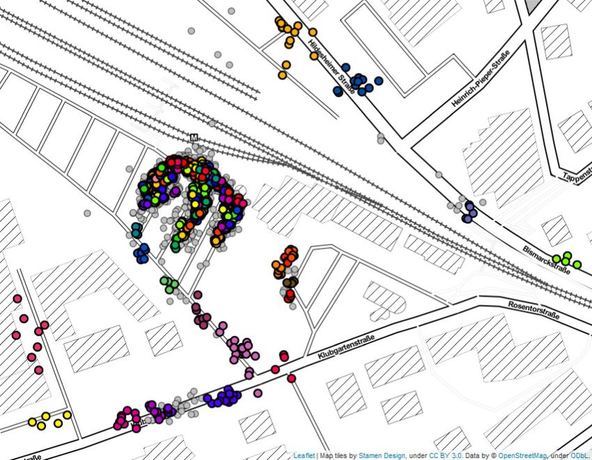
extraction method [2] [11]. HDBSCAN was proposed as                linkage algorithm by Chaudhuri et al. [16]. A detailed
an improved extension of DBSCAN and OPTICS for data                explanation of the relationships between those approaches
exploration in diverse research fields. It has an efficient        and HDBSCAN is provided by McInnes and Healy [11].
Python implementation [12] that conforms to the scikit-               Starting from the root, HDBSCAN regards each cluster
learn [13] library and supports a variety of metrics. The          split as a true split only if both child clusters contain at
algorithm requires only a minimum cluster size as user input       least minP ts objects. If they both contain less than minP ts
and then simplifies a complex single-linkage hierarchy to a        objects, the cluster is considered as having disappeared at
smaller tree of candidate clusters. A flat solution is extracted   this density level. If only one of the children has less than
automatically based on local cuts. In [14], Campello et al.        minP ts objects, the interpretation is that the parent cluster
introduce the “Framework for Optimal Selection of Clusters”        has simply lost points but still exists. “Lost” points are
(FOSC) that formalizes cluster selection through local cuts        regarded as noise. This simplification process results in a
as an optimization problem. HDBSCAN’s original selection           hierarchy of candidate clusters at different density levels.
approach is an example of a FOSC-compliant method.
                                                                   C. Stability-based Cluster Selection
   The method proposed in this paper – HDBSCAN(ˆ         ) – is
intended as an alternative cluster selection approach for the         Given the condensed cluster tree, one possibility is to
HDBSCAN hierarchy. By implementing it in compliance to             simply select all leaf nodes. These are the clusters with
FOSC, it can easily be combined with other FOSC methods,           lowest epsilon values in the hierarchy, and represent clusters
and setting the threshold to 0 always results in the same          that cannot be split up any further with respect to minP ts.
clustering as the original HDBSCAN. We will give a brief           This selection method is one of two provided options in
overview of HDBSCAN and FOSC in the following section.             HDBSCAN’s Python implementation – from now on called
                                                                   HDBSCAN(leaf) – and results in very fine-grained clusters.
            III. T HE HDBSCAN A LGORITHM                              The other option is eom, short for excess of mass. This
   HDBSCAN is built on top of a slightly modified version of       method is recommended by Campello et al. [2] as the optimal
DBSCAN, called DBSCAN*, which declares border points               global solution to the problem of finding clusters with the
as noise [2]. Unlike DBSCAN(*), HDBSCAN does not select            highest stability, which they define as
clusters based on a global epsilon threshold, but creates                              X
                                                                            S(Ci ) =       (λmax (xj , Ci ) − λmin (Ci ))
a hierarchy for all possible epsilon values with respect to
                                                                                           xj ∈Ci
minP ts as minimum cluster size.                                                                                                       (1)
                                                                                            X                 1            1
                                                                                    =               (                  −           )
A. Mutual Reachability Distance                                                                         min (xj , Ci ) max (Ci )
                                                                                           xj ∈Ci
   In HDBSCAN, the core distance dcore is defined as the
distance of an object to its minPts-nearest neighbor. The             where the density value λ is simply set to 1 . This
constructed hierarchy is based on the mutual reachability          means that λ values become larger from root towards leaves,
distance, which for two objects xp , xq is                         whereas the corresponding  distance values become smaller.
                                                                   Subtracting λmin (Ci ), which corresponds to the density level
           max{dcore (xp ), dcore (xq ), d(xp , xq )}              at which cluster Ci first appears, from the value beyond
                                                                   which object xj ∈ Ci no longer belongs to Ci , results in
where d(xp , xq ) refers to the “normal” distance according
                                                                   a measure of lifetime for xj . The sum of all object lifetimes
to the chosen metric, e.g. Euclidean distance. This approach
                                                                   within Ci leads to the overall cluster lifetime S(Ci ), which
separates sparse points from others by at least their core
                                                                   is called stability because the clusters with longest lifetimes
distance and makes the clustering more robust to noise.
                                                                   are considered to be the most stable ones.
   The data set can then be represented as a graph with data          The authors then formalize an optimization problem for
objects as vertices, connected by weighted edges with the          maximizing the sum of these cluster stabilities as
mutual reachability distances as weights. Using this graph
to construct a minimum spanning tree and sorting its edges                                      k
                                                                                                X
by mutual reachability distance results in a hierarchical tree                 max J =                    δi S(Ci )
                                                                              δ2 ,...,δk
structure (dendrogram). By choosing an epsilon as a global                                     (    i=2
                                                                                                                                       (2)
horizontal cut value and selecting all clusters with at least                                       δi ∈ {0, 1}, i = 2, ..., k
minP ts points at this density level, we could retrieve the                   subject to            P
                                                                                                       j∈Ih δj = 1, ∀h ∈ L
DBSCAN* clusters for this epsilon from the hierarchy.
                                                                   with L = {h|Ch is leaf cluster} as leaves, Ih as the set of
B. Condensed Cluster Hierarchy                                     clusters on the paths from leaves to the excluded root, and δi
  Since HDBSCAN aims at discovering clusters of variable           as boolean indicator whether the respective cluster is selected
densities, it instead proceeds to building a simplified version    or not. The definition ensures that no more than one cluster
of the complex hierarchy tree, the condensed cluster tree.         can be selected on any branch from leaf towards root.
This approach follows the tree pruning concept of which               To solve this problem, HDBSCAN’s selection algorithm
many variants exist in literature, such as runt pruning by         traverses the cluster tree bottom-up. The stability value of
Stuetzle [15] or pruning a tree created by a robust single         each node is compared to the sum of stability values of its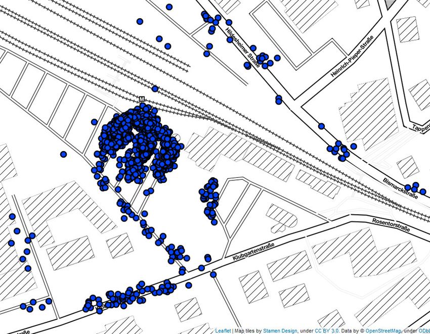
nested subclusters. In this way, stabilities are propagated and
updated when going up the tree until the cluster with highest
stability is found and selected on each branch.

D. Framework for Optimal Selection of Clusters
   The excess of mass (eom) method for cluster extraction
as explained above conforms to the generic “Framework
for Optimal Selection of Clusters” (FOSC) introduced by
Campello et al. [14]. FOSC requires two essential properties:
First, the chosen measure for cluster selection – in this case,           (a) The sample data set           (b) HDBSCAN with minP ts = 4
the stability criterion – must be local, i.e. it can be computed
for each cluster independently of other selected clusters.
Second, it must be additive, i.e. it must be meaningful to
add up the computed cluster values (in this case, cluster
stabilities) so that an optimization problem as shown above
can be formulated as maximizing the sum of values. More-
over, it must be ensured that exactly one cluster is selected
on each branch. This formal problem can then be solved
by traversing the hierarchy tree bottom-up starting from the
                                                                      (c) OPTICS with minP ts = 4,         (d) DBSCAN* with minP ts = 4,
leaves, deciding for each candidate cluster whether it should                   ξ = 0.05                             = 5 meters
be part of the final solution. FOSC thus provides an efficient
                                                                      Fig. 1.   Clustering results for a sample data set of GPS locations.
way of finding the globally optimal solution for the extraction
of clusters according to the chosen measure.

            ): A T HRESHOLD FOR C LUSTER S PLITS
IV. HDBSCAN(ˆ                                                      not bound to collective pick-up or drop-off locations, even
                                                                   small groups of 4 or 5 points are of interest to us.
   In this section, we introduce an approach for selecting
clusters from the HDBSCAN hierarchy based on a distance               Figure 1b presents the clustering result with HDBSCAN’s
threshold ˆ. Our motivation for this approach is given below,     default selection method eom, from now on referred to
followed by a formal definition.                                   as HDBSCAN(eom). Using minP ts = 4, the algorithm
                                                                   successfully discovers all the small clusters while declaring
A. Motivation                                                      obvious outliers or groups with less than 4 points as noise
   HDBSCAN is a powerful clustering algorithm for unsu-            (gray points). However, in the high-density area around the
pervised data exploration. However, for some applications,         train station, it generates a very large number of micro-
the single input parameter minP ts might not be sufficient         clusters. In our case, this is not what we want: we would
to discover the clusters that best represent the underlying        prefer one or only few clusters representing the location. This
data structure. In particular, let us consider a large data set    would be possible by increasing minP ts, but at the cost of
distributed such that there is a high number of very dense         losing small clusters in less dense areas or merging them
objects in some areas, and only few objects in other areas.        into other clusters separated by a relatively large distance.
If we were only interested in the highly populated areas,             We clustered the same data set with OPTICS from scikit-
HDBSCAN would give us good results for a minP ts value             learn and DBSCAN* from HDBSCAN’s Python implemen-
large enough to declare sparse regions as noise and dense          tation. The minP ts parameter was set to 4 in both cases.
regions as clusters. In some cases, however, we do not want        For OPTICS, we tried ξ values between 0.03 to 0.05, and
all observations in sparse environments to be marked as            for DBSCAN*, we tried  values between 3 and 10 meters
noise: these areas might naturally contain fewer objects, but      (haversine distance). In each case, we chose a value that in-
small yet dense groups of objects that do exist might be just      tuitively produces the best results. Figure 1c shows OPTICS
as relevant as the ones in regions with lots of data.              clusters for ξ = 0.05, which are similar to HDBSCAN.
   Figure 1a demonstrates such a scenario. It shows around         Figure 1d depicts DBSCAN* results for  = 5 meters, which
2800 GPS data points on a map extract, representing                seems clearly better suitable for our application. However,
recorded pick-up and drop-off locations from a door-to-door        DBSCAN* neglects potentially important clusters with den-
demand-responsive ride pooling system [17]. Our aim was            sities beyond the chosen threshold. In particular, this applies
to assign addresses requested by customers to the closest          to the two groups of objects on the bottom-left and another
areas where ride pooling vehicles were actually able to            two on the far-right. A larger  would cover these objects,
stop in the past, i.e. in compliance with traffic rules and        but at the same time merge other clusters. Note that this
available space. The largest (visual) data cluster can be found    demonstration is based on only a small sample. Applying
around the train station. Smaller clusters are placed along        DBSCAN(*) to a larger data set increases its tendency to
the streets, depending on the requested location. Since we         single-linkage effects when increasing , such as extending
are considering a door-to-door system where customers are          the largest cluster down the streets.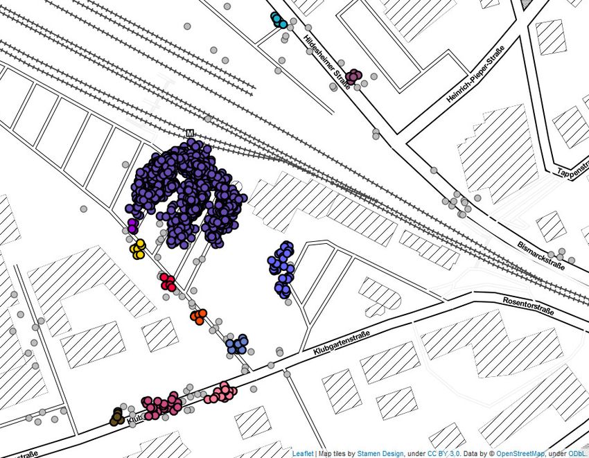
For a scenario like this, a combination between                     Algorithm 1: Solution to the Optimization Problem
HDBSCAN and DBSCAN* would be useful. The essential
                                                                         1. Initialize δ(.) = 1 for all leaves
idea is that instead of performing a cut through the entire
                                                                         2. Do bottom-up from all leaves (excluding the root):
hierarchy, we just prevent clusters below a given threshold
from splitting up any further. We could then still select                   2.1. If ES(Ci ) > 0 or δCi = 0, continue to next leaf
regular HDBSCAN clusters from data partitions not affected                  2.2. Else if ES(Ci ) = 0 and ES(CP AREN T (i) ) > 0,
by the threshold. All others would be DBSCAN* clusters.                           set δP AREN T (i) = 1 and set δ(.) = 0 for all
                                                                                  nodes in CP AREN T (i) ’s subtree
B. Formal Definition
   We define the application of a threshold to the HDBSCAN
hierarchy as a selection method in accordance with the
framework FOSC [14] as explained earlier. To formalize our                          0.02                                   0.02
cluster selection criterion, we introduce the notions of epsilon
stable and epsilon stability.                                               0.03                0.03               0.03              0.03
   Definition 1 (Epsilon stable): A cluster Ci with i =
{2, ..., k} is called epsilon stable if max (Ci ) > ˆ for a given                0.05                1.4                0.05              0

ˆ > 0.
   As explained earlier, λmin (Ci ) = max1(Ci ) is the density                           0.3                                    0

level at which cluster Ci appears. Note that this is equal to the
level at which it split off its parent cluster. Hence we call a                                  0.6                                   0

cluster epsilon stable if the split from its parents occurred at a      (a) Hierarchy with λmin                 (b) Hierarchy with ES values
distance above our threshold ˆ (or below the level λmin (Ci ),         values per level                        for λ = 0.2
respectively) and formally define epsilon stability as follows:       Fig. 2. The cluster tree in Figure 2a is annotated with the λmin value
   Definition 2 (Epsilon Stability):                                  per hierarchy level. Figure 2b shows the same tree annotated with epsilon
                                                                      stability values for a given threshold ˆ = 5 (or λ = 0.2, respectively). On
                     (                                                each path, the cluster with maximum epsilon stability is highlighted in red.
                       λmin (Ci ) if Ci is epsilon stable
        ES(Ci ) =
                       0            otherwise
                                                                      reaching the root, we select it as a cluster and unselect all
   If we select the cluster with highest epsilon stability on         of its descendants.
each path of the HDBSCAN condensed hierarchy tree, we                    Since ES(Ci ) decreases as we traverse up the tree (unless
end up with all the clusters that we do not want to split up any      for 0 values), this procedure ensures that we are selecting the
further w.r.t. ˆ and minP ts. Their parents split up at some         maximum epsilon stable cluster on each path. This is equal
distance min > ˆ, which is equal to the max value on the           to selecting the first cluster on the path that “was born” at a
level where their children appear. While those children are           distance greater than ˆ and is thus not allowed to split up.
still valid clusters, they are not allowed to split up themselves        The concept is illustrated in Figure 2, which shows the
                                                              1
because either they are leaf clusters or the level λmax = min        cluster tree for a small sample data set. The tree on the left
at which the split would happen is above the threshold.               is annotated with λmin values. On the right, the same tree
   Given these definitions, we can formulate the optimization         is annotated with corresponding epsilon stability values for
problem that maximizes the sum of epsilon stabilities in the          ˆ = 5 meters, or λ = 1ˆ = 0.2. According to Definition 2,
same way as previously shown in Section III-C (Problem 2),            each cluster on a level that is not epsilon stable is set to 0.
with the only difference that we replace S(Ci ) with ES(Ci ).         All others receive their λmin as epsilon stability value.
The definition ensures that we extract only the maximum                  It can be seen that the density levels with λmin values of
epsilon stable cluster on each path from leaf towards root.           0.6, 0.3 and 1.4 exceed the threshold of 0.2. This indicates
                                                                      that the parents of clusters on these levels split up at a
C. Selection Algorithm                                                distance lower than 5 meters. By starting from the leaves
   The original selection algorithm by Campello et al. [2]            and selecting the ascendant with maximum epsilon stability
takes into account that the total stability value needs to be         value on each path, we receive the final set of clusters
updated at each step. In our case, this is not necessary due          (highlighted in red). Note that instead of starting from the
to the definition of epsilon stability. The pseudo code in            leaves, we could optionally also start with the nodes selected
Algorithm 1 thus shows a simplified version of the original           by HDBSCAN(eom). This would combine both methods, i.e.
code that has been adapted to our problem. First, we mark             after selecting the most stable clusters we could still decide
all leaves of the HDBSCAN cluster hierarchy as selected.              to merge clusters up to the given threshold value.
If a leaf has previously been marked as not being a cluster,             HDBSCAN(ˆ    ) can be viewed as FOSC-compliant: the ES
or if it is already epsilon stable (i.e., λmin
(a) HDBSCAN(eom) (b) OPTICS with ξ = 0.05
(a) DS1 (b) DS2
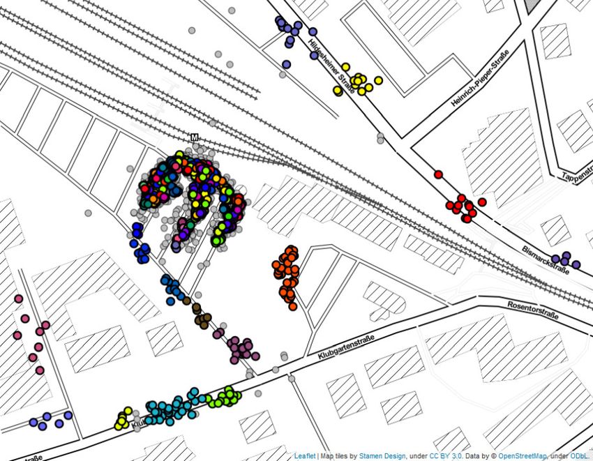
Fig. 3. A synthetic data set (left) and a real data set (right).
V. E XPERIMENTS AND D ISCUSSION
Before applying HDBSCAN(ˆ ) to the GPS data set intro-
duced in Section IV-A, we also demonstrate the algorithm
on a synthetic data set and an alternative real data set as
illustrated in Figure 3. Different (random) colors represent (c) DBSCAN* with = 0.34 ) with ˆ = 0.1
(d) HDBSCAN(ˆ
the true labels. Both data sets contain clusters of variable Fig. 4. Clustering results for DS1. Colorless points are noise.
shapes and densities and serve as examples for cases where
HDBSCAN(eom) alone leads to an abundance of micro-
clusters. For comparison, each data set was also clustered
with OPTICS and DBSCAN*. Since we focus on scenarios
where we require a low minimum cluster size, minP ts was
set to 4 for DS1 and 2 for DS2. Epsilon in DBSCAN* and
HDBSCAN(ˆ ) was in each case set to a value that results
in the most accurate clustering w.r.t. the ground truth data.
OPTICS’ ξ value was set to 0.05 in both cases. Lower or
(a) HDBSCAN(eom) (b) OPTICS with ξ = 0.05
higher values did not improve the result.
Figure 4 shows that HDBSCAN(eom) discovers clusters of
variable densities in DS1, but breaks up high-density regions
into micro-clusters. OPTICS results are no improvement over
HDBSCAN(eom). DBSCAN* almost achieves the desired
output, but we could not find an epsilon value that recognizes
the cluster on the bottom-left while keeping the remaining
clusters separated. Figure 4c shows the result for = 0.34,
which is just large enough not to merge clusters and at the (c) DBSCAN* with = 0.13 ) with ˆ = 0.1
(d) HDBSCAN(ˆ
same time not declaring any more points as noise. Fig. 5. Clustering results for DS2. Colorless points are noise.
DS2 is based on radar data from nuscenes [18] (scene-
0553) with reflections from pedestrians and vehicles. In Fig-
ure 3b, the ego vehicle position is marked with a red arrow, for DBSCAN* and 0.1 - 0.38 (DS1) and 0.04 - 0.35 (DS2)
and bounding boxes for moving objects are included. Note for HDBSCAN(ˆ ). This indicates that HDBSCAN(ˆ ) is less
that the manually chosen “true” labels consider the group sensitive to the choice of its epsilon parameter.
of pedestrians (red points) as one cluster, but results that Results are represented by the Adjusted Rand Index (ARI)
detect subgroups would also be acceptable. Potential clutter as seen in Table I. Note that the ARI, a commonly used
and stationary objects below a threshold of 0.1 m s were
cluster validation measure, does not consider noise. Hence,
removed. By clustering based on a 3D data set where Doppler DBSCAN* and HDBSCAN(ˆ ) both achieve a perfect ARI
velocity and Cartesian x/y coordinates were scaled to values score of 1 for DS1, although DBSCAN* marks the bottom-
between 0 and 1, we used a very simple radar clustering left cluster as noise. For DS2, we recorded DBSCAN*’s
approach. However, the example again demonstrates that for perfect score for = 0.13 instead of the result for = ˆ.
a low minP ts, OPTICS and HDBSCAN(eom) might create Finally, we applied HDBSCAN(ˆ ) to the sample of GPS
undesired micro-clusters (see Figure 5). For DBSCAN*, an data introduced in Section IV-A. Figure 6 shows the result
epsilon lower than 0.13 neglects relevant reflections from for ˆ = 5 meters. Compared to DBSCAN* in Figure 1d with
the pedestrian group. For larger values, a perfect result can the same epsilon value, and HDBSCAN(eom) in Figure 1b,
be achieved. However, larger epsilons increase the risk of we notice that we indeed receive a combination of both.
merging other clusters, e.g. vehicles driving side by side. We no longer lose clusters of variable densities beyond the
In contrast, HDBSCAN(ˆ ) does not require an ˆ larger than given epsilon, but avoid the high number of micro-clusters in
0.1. Overall, the range of possible epsilon values for the the original clustering, which was an undesired side-effect of
best result are 0.34 - 0.38 (DS1) and 0.13 - 0.35 (DS2) having to choose a low minP ts value. Note that for the givenTABLE I We belief that this extension will prove to be valuable
C LUSTERING RESULTS FOR DATA SET DS1 AND DS2 IN TERMS OF particularly in clustering spatial data, but it could also be
A DJUSTED R AND I NDEX (ARI) AND PERCENTAGE OF DATA POINTS NOT applied to different kind of data. Future work might include
MARKED AS NOISE (% C ). HDB. IS SHORT FOR HDBSCAN. combinations with further selection methods such as semi-
supervised approaches.
Data HDB. (eom) OPTICS DBSCAN* HDB. )
(ˆ
Set ARI %c ARI %c ARI %c ARI %c R EFERENCES
DS1 0.28 0.75 0.11 0.78 1 0.98 1 1 [1] H.-P. Kriegel, P. Kröger, J. Sander, and A. Zimek, “Density-based clus-
DS2 0.80 0.92 0.09 0.90 1 1 1 1 tering,” Wiley Interdisciplinary Reviews: Data Mining and Knowledge
Discovery, vol. 1, no. 3, pp. 231–240, 2011.
[2] Campello, Ricardo J. G. B. and Moulavi, Davoud and Sander, Joerg,
“Density-based clustering based on hierarchical density estimates,”
in Advances in Knowledge Discovery and Data Mining. Berlin,
Heidelberg: Springer Berlin Heidelberg, 2013, pp. 160–172.
[3] M. Ester, H.-P. Kriegel, J. Sander, and X. Xu, “A density-based
algorithm for discovering clusters a density-based algorithm for dis-
covering clusters in large spatial databases with noise,” in Proceedings
of the Second International Conference on Knowledge Discovery and
Data Mining, ser. KDD’96. AAAI Press, 1996, pp. 226–231.
[4] A. Rodriguez and A. Laio, “Clustering by fast search and find of
density peaks,” Science, vol. 344, no. 6191, pp. 1492–1496, 2014.
[5] Y. Zhu, K. M. Ting, and M. J. Carman, “Density-ratio based clustering
for discovering clusters with varying densities,” Pattern Recognition,
vol. 60, pp. 983 – 997, 2016.
[6] M. Ankerst, M. M. Breunig, H.-P. Kriegel, and J. Sander, “OPTICS:
Ordering points to identify the clustering structure,” in Proceedings
Fig. 6. ) with minP ts = 4, ˆ = 5 meters
HDBSCAN(ˆ of the 1999 ACM SIGMOD International Conference on Management
of Data, ser. SIGMOD ’99. New York, NY, USA: Association for
Computing Machinery, 1999, p. 49–60.
parameter setting, running HDBSCAN(ˆ ) based on eom or [7] J. Sander, X. Qin, Z. Lu, N. Niu, and A. Kovarsky, “Automatic
leaf would not make any difference: ˆ neutralizes the effect extraction of clusters from hierarchical clustering representations,”
in Proceedings of the 7th Pacific-Asia Conference on Advances in
of HDBSCAN’s stability calculation. For a lower threshold, Knowledge Discovery and Data Mining, ser. PAKDD ’03. Berlin,
e.g. ˆ = 3, some minor differences can be noticed. Heidelberg: Springer-Verlag, 2003, pp. 75–87.
[8] A. Dockhorn, C. Braune, and R. Kruse, “An alternating optimization
In general, the most suitable ˆ value is certainly not always approach based on hierarchical adaptations of DBSCAN,” in 2015
easy to choose. For GPS data, it is quite intuitive to decide IEEE Symposium Series on Computational Intelligence, Dec 2015,
on a distance threshold, but in higher-dimensional data, this pp. 749–755.
[9] A. Dockhorn, C. Braune, and R. Kruse, “Variable density based clus-
becomes more difficult. Another limitation of our method is tering,” 2016 IEEE Symposium Series on Computational Intelligence
that cutting the hierarchy at a fixed threshold can neglect (SSCI), pp. 1–8, 2016.
meaningful subclusters. Hence, it inherits DBSCAN(*)’s [10] G. Gupta, A. Liu, and J. Ghosh, “Automated hierarchical density shav-
ing: A robust automated clustering and visualization framework for
shortcomings wherever it uses a fixed value to select clusters. large biological data sets,” IEEE/ACM Transactions on Computational
It could also be argued that the threshold could already be Biology and Bioinformatics, vol. 7, no. 2, pp. 223–237, April 2010.
applied when building the hierarchy and does not require the [11] L. McInnes and J. Healy, “Accelerated hierarchical density based
clustering,” in 2017 IEEE International Conference on Data Mining
definition of an optimization problem or FOSC-compatibility. Workshops (ICDMW), Nov 2017, pp. 33–42.
However, the application at selection stage has the major [12] L. McInnes, J. Healy, and S. Astels, “hdbscan: Hierarchical density
advantage that we do not need to modify HDBSCAN’s based clustering,” The Journal of Open Source Software, vol. 2, no. 11,
mar 2017.
original hierarchy and then re-build it every time we apply [13] F. Pedregosa, G. Varoquaux, A. Gramfort, V. Michel, B. Thirion,
a different threshold. Instead, we can work with the original O. Grisel, M. Blondel, P. Prettenhofer, R. Weiss, V. Dubourg, J. Van-
tree (or even a cache) and then efficiently explore our data derplas, A. Passos, D. Cournapeau, M. Brucher, M. Perrot, and
E. Duchesnay, “Scikit-learn: Machine learning in Python,” Journal
set with different selection methods and thresholds. It has of Machine Learning Research, vol. 12, pp. 2825–2830, 2011.
been shown that FOSC cluster extraction does not increase [14] R. J. G. B. Campello, D. Moulavi, A. Zimek, and J. Sander, “A
the overall complexity of HDBSCAN, which is O(n2 ) [14]. framework for semi-supervised and unsupervised optimal extraction
of clusters from hierarchies,” Data Mining and Knowledge Discovery,
VI. S UMMARY AND C ONCLUSION vol. 27, no. 3, pp. 344–371, Nov 2013.
[15] W. Stuetzle, “Estimating the cluster tree of a density by analyzing the
We introduced the cluster selection method HDBSCAN(ˆ ) minimal spanning tree of a sample,” Journal of Classification, vol. 20,
that applies a distance threshold to HDBSCAN’s hierar- no. 1, pp. 025–047, May 2003.
[16] K. Chaudhuri, S. Dasgupta, S. Kpotufe, and U. von Luxburg, “Con-
chy and therefore acts like a hybrid between DBSCAN* sistent procedures for cluster tree estimation and pruning,” IEEE
and HDBSCAN: for data partitions affected by the given Transactions on Information Theory, vol. 60, no. 12, pp. 7900–7912,
threshold ˆ, we extract DBSCAN* results, for all others 2014.
[17] N. Avermann and J. Schlüter, “Determinants of customer satisfaction
HDBSCAN clusters. The method is designed to be compati- with a true door-to-door DRT service in rural Germany,” in Research in
ble to the framework FOSC and can be combined with other Transportation Business & Management, vol. 32, 2019, paper 100420.
FOSC-compliant methods. It can easily be integrated into ex- [18] H. Caesar, V. Bankiti, A. H. Lang, S. Vora, V. E. Liong, Q. Xu, A. Kr-
ishnan, Y. Pan, G. Baldan, and O. Beijbom, “nuscenes: A multimodal
isting HDBSCAN implementations and is already available dataset for autonomous driving,” arXiv preprint arXiv:1903.11027,
as part of the scikit-learn compatible Python module [12]. 2019.You can also read