AUTOMATED STRUCTURAL FOREST CHANGES USING LIDAR POINT CLOUDS AND GIS ANALYSES
←
→
Page content transcription
If your browser does not render page correctly, please read the page content below
The International Archives of the Photogrammetry, Remote Sensing and Spatial Information Sciences, Volume XLIII-B3-2021
                                                XXIV ISPRS Congress (2021 edition)

   AUTOMATED STRUCTURAL FOREST CHANGES USING LiDAR POINT CLOUDS
                        AND GIS ANALYSES

                 A. Novo1 *, H. González-Jorge2, J. Martínez-Sánchez1, José María Fernández-Alonso3, H. Lorenzo4
  1. Geotech-Group,  CINTECX, Department of Natural Resources and Environmental Engineering School of Mining Engineering,
                          University of Vigo, 36310, Vigo, Spain - (annovo, joaquin.martinez)@uvigo.es
   2 Physics Engineering Lab, School of Aerospace Engineering, University of Vigo, 32004, Ourense, Spain – higiniog@uvigo.es
      3 Lourizán Forest Research Center Xunta de Galicia, P.O. Box 127, 36080 Pontevedra, Spain – josemfernandez@uvigo.es
 4 Geotech-Group, CINTECX, Department of Natural Resources and Environmental Engineering, School of Forestry Engineering,

                                University of Vigo, 36005 Pontevedra, Spain – hlorenzo@uvigo.es

                                                     Commission III, WG III/10

KEY WORDS: Mapping, Remote Sensing, LiDAR data, GIS analysis, Point cloud processing, Vegetation structure, Forest
           parameters.

ABSTRACT:

Forest spatial structure describes the relationships among different species in the same forest community. Automation in the
monitoring of the structural forest changes and forest mapping is one of the main utilities of applications of modern geoinformatics
methods. The obtaining objective information requires the use of spatial data derived from photogrammetry and remote sensing. This
paper investigates the possibility of applying light detection and ranging (LiDAR) point clouds and geographic information system
(GIS) analyses for automated mapping and detection changes in vegetation structure during a year of study. The research was
conducted in an area of the Ourense Province (NWSpain). The airborne laser scanning (ALS) data, acquired in August 2019 and
June of 2020, reveal detailed changes in forest structure. Based on ALS data the vegetation parameters will be analysed.
To study the structural behaviour of the tree vegetation, the following parameters are used in each one of the sampling areas: (1)
Relationship between the tree species present and their stratification; (2) Vegetation classification in fuel types; (3) Biomass (Gi); (4)
Number of individuals per area; and (5) Canopy cover fraction (CCF). Besides, the results were compared with the ground truth data
recollected in the study area.
The development of a quantitative structural model based on Aerial Laser Scanning (ALS) point clouds was proposed to accurately
estimate tree attributes automatically and to detect changes in forest structure. Results of statistical analysis of point cloud show the
possibility to use UAV LiDAR data to characterize changes in the structure of vegetation.

                    1. INTRODUCCTION                                   structural diversity metrics can be estimated using methods that
                                                                       range from traditional forest inventory approaches to next-
Forest constitutes the most biologically diverse terrestrial           generation remote sensing techniques (Fahey et al. 2019). The
ecosystem on Earth and are imperative for maintaining the              complex and dynamic nature of forest structure has proven to be
balance of terrestrial ecosystems (Dandois, Olano, and Ellis           challenging to measure accurately across scales and forest
2015). To promote and support sustainable forest management            structure types (Atkins et al. 2018).
an accurate monitoring in timely fashion is required (Timilsina
et al. 2013). In this context, forest structural parameters (e.g.,     The forestry management process is based on the use of a large
tree height, volume, and biomass) are key components for               amount of information which must be stored, managed,
effectively quantifying forest structure and are vital for             analyzed, simulated, and visualized in a dynamic and flexible
accurately monitoring forest dynamics (Fu et al. 2021).                way. Geographic Information Systems (GIS) and remote
Assessing changes in forest structure over time is crucial for         sensing are complementary technologies that, when combined,
monitoring forest resources. The generation of spatially explicit      enable to improve monitoring, mapping and management of
detailed maps of forest structure, and its dynamics, has multiple      forest resources (S. E. Franklin 2001).
implications in forest managing wildfire risk reduction, carbon
sequestration assessment, timber resources availability or             Automation in the monitoring of the structural forest changes
wildfire habitat analysis may benefit from such high-resolution        and forest mapping is one of the main aspects of applications of
information. Forest structural diversity is the physical               modern geoinformatics methods. The obtaining of objective
arrangement and variability of the living and non-living biotic        information requires the use of spatial data derived from
elements within forest stands that support many essential              photogrammetry and remote sensing. Generating the spatial
ecosystem functions (LaRue et al. 2019). Forest structural             characteristics of vegetation in an automated way undoubtedly
diversity arises from the complex interactions of a range of           provides new possibilities in modelling the structure of
abiotic and biotic factors that influence the growth and the           vegetation, including defining biometric features and biomass,
quality of vegetation (Fotis et al. 2018). A wide variety of

* Corresponding author

                                                This contribution has been peer-reviewed.
                 https://doi.org/10.5194/isprs-archives-XLIII-B3-2021-603-2021 | © Author(s) 2021. CC BY 4.0 License.                 603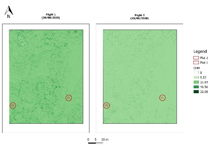
The International Archives of the Photogrammetry, Remote Sensing and Spatial Information Sciences, Volume XLIII-B3-2021
                                                XXIV ISPRS Congress (2021 edition)

which determines the developmental stage of trees and shrubs              -          Analyse the forest changes in the whole study
forming the succession process. Information about the spatial                  area, supported by hight parameters, biomass
structure of vegetation provides a basis for studies of                        estimation, individual tree detection, CCF and fuel
biodiversity, or spatial analyses that require up to date and                  types of classification.
precise information about land cover classes (Szostak 2020).

Remote sensing has demonstrated its importance for the                             2. MATERIAL AND METHODS
characterization of vegetation structure in sparsely dense
forests, the greatest challenge being those with medium-high         2.1 Area of study
density (J. Franklin 2010). Light Detection and Ranging
(LiDAR) is a remote sensing technology for characterizing the        The study area is located in the northwest of Spain. It belongs to
surface of the earth using a cloud of georeferenced points.          the Natural Park of Baixa Limia Serra do Xurés, which has been
LiDAR is a useful tool for the multi-dimensional                     catalogued as an Area for Special Conservation (ASC). The
characterization of forest structure because it has a strong         protected areas are ideal settings for research. The subject of
capability to penetrate dense forest canopies and detect             study is an area of 0.30 Ha in the central part of the municipality
understory vegetation, thereby, obtaining high-precision three-      of Lobios (Figure 1). The study area contains two sampling
dimensional (3D) forest structure information. Over more, there      subareas corresponding to the ground truth data. One four
are versatile terrestrial and aerial deployment platforms.           square meter plot was stablished in each subarea to carry out
Terrestrial laser scanning (TLS) and aerial laser scanning (ALS)     field-based data collection. The climatic type existing in the
have both been shown to be effective at quantifying components       Baixa Limia is called sub-Mediterranean oceanic temperate,
of forest structural diversity (LaRue et al. 2020). The              which indicates a certain aridity during summer. This means
development of airborne digital cameras and unmanned aerial          that a large part of vegetation is adapted to dry periods. Under
vehicles (UAV) has promoted cost-effective methods for               this climatic type, the potentially dominant vegetation in most
enhancing monitoring forest dynamics. In the forest sector,          of the territory is Quercus pyrenaica and Quercus robur. The
LiDAR has the potential to reduce the need for intensive             main tree species are, Betula alba, Quercus suber, Arbutus
ground-based measurement of stand structure, making it a             unedo, Pinus sp., Ulex sup, Cytisus scoparius and Erica sp.
valuable tool. LiDAR data have been recently used to quantify        These are several endemic plants, including Portugal laurel and
complexity and diversity in vegetation structure in a successful     Prunus lusitanica, a species that colonizes the ravines and other
way (Atkins et al. 2018; Bakx et al. 2019; Guo et al. 2017;          areas that have high humidity. The biogeographical location of
LaRue et al. 2020).                                                  Baixa Limia greatly favours the diversity of the flora in this
                                                                     territory.
The present manuscript explores the accuracy of airborne
LiDAR data to support, automatically map, and monitoring the
forest structural changes, in a more efficient way than
traditional forest methods do such as human field data
collection.

The aim of this work is to analyze the potential of automated
mapping and detection changes in vegetation structure using
LiDAR technology and Geographic Information System (GIS)
analyses. In this way, human work would not be necessary for
field data collection and the methodology could be extended to
large or inaccessible areas, being able to map and analyze the
vegetation evolution whose data are necessary in forest
management. Firstly, the LiDAR data are collected with a year
of difference between first and second flight. Moreover, the
ground truth collected by human methods coincide with the
second fly date. Then, data are recollected in two square plots of
2 m size within the study area. The LiDAR data are processed                         Figure 1. Location of study area.
to be compared with ground truth data and the results accuracy
is calculated in both study plots. Finally, the methodology is       2.2 Materials
extended to the whole study area, and combustible fuel types
and their evolution are mapped. In particular, the main              The experimental data for this work were collected using a
contributions of this study are summarized as:                       Phoenix system, which is based on a Velodyne LiDAR model,
                                                                     the Alpha AL3-32. It shows survey-grade centimetric accuracy
     -          Design of a methodology to group tree points by      and intensity calibration. Their 32 lasers emit 700,000 pulses
          height, Prometheus classification, and heights             per second and record up to two returns per pulse. The system
          established in ASPRS classification.                       includes a global navigation satellite system (GNSS) that
                                                                     provides real-time kinematics and post-processing options with
     -          Development of an algorithm to automatically         an accuracy specification up to 1cm in horizontal and 2.5 cm in
          calculate the height distribution of vegetation and        vertical positioning. The raw point cloud of the first flight was
          their Canopy Cover Fraction (CCF).                         collected on 30th August 2019 and the second flight was
                                                                     performed on 25th June 2020. Data were collected with a density
     -        Calculate the accuracy of the methodology              of 350 points/m2 and an average point spacing of 0.05 m. The
          compared with the one for the ground truth.                point cloud collected in 2019 is composed by a total of
                                                                     1,074,390 points, while the total points of the 2020 point cloud
                                                                     are 705,852.

                                                This contribution has been peer-reviewed.
                 https://doi.org/10.5194/isprs-archives-XLIII-B3-2021-603-2021 | © Author(s) 2021. CC BY 4.0 License.               604
The International Archives of the Photogrammetry, Remote Sensing and Spatial Information Sciences, Volume XLIII-B3-2021
                                                XXIV ISPRS Congress (2021 edition)

ALS point clouds were first preprocessed filtering vegetation
points using the command Lasground from the LAStools
software (Isenburg 2012). This process was done to remove the
noise and ground points. Then, data were normalized by using
the command Lasheight.

In this work, filed based inventory data are used as ground truth
for their comparison with the LiDAR data. The ground truth
data were collected in two subareas within the study area. Plot 1
has an average “x” and “y” coordinates of 574037.3 m and
4633978.6 m, respectively. Plot 2 shows an average “x”
coordinate of 573999.4 m and “y” coordinate of 4633973.3 m.
In both cases EPSG:25829 ETRS89/UTM zone 29N.

That validation data was collected by setting a four-square
meters plot. For the computational analyses, a two-meter ratio
influence area (buffer) was generated around each plot taking
the average “x” and “y”coordinates as reference. The field data
collection consisted of the characterization of canopy surface
fuel strata. For the canopy strata, top canopy height, height of     Figure 2. Classification of vegetation points in both plots study
living crown and canopy closure were recorder. A Haglöf
Vertex Hypsometer was used to measure vertical heights. This         Once the vegetation was grouped by height the statistical
instrument uses ultrasonic signals to obtain the distance. For the   variables were calculated by GIS static analysis. The average
surface fuel stratum, a quadrat sampling method was applied,         height for each established vegetation stratum has been
where height and coverage measurements were taken each 25            calculated, as well as for the entire vegetation in both years of
cm. Average height of ligneous species (shrubs), coverage of         study. In addition, the subtraction of heights in both years gives
herbaceous species, coverage of shrubs and percentage of plot        the characteristics of evolution and changes in the forest
without vegetation cover was derived from that sampling. Each        structure both in total area and in study plots.
sampling plot was classified according to Prometheus fuels
classification according to measured data and visual inspection.     The CCF has been calculated for each stratum of vegetation and
                                                                     for the entire vegetation in both years of study. The CCF
2.3 Data processing                                                  indicates the proportion of ground covered by vertical
                                                                     projection of each vegetation stratum. Figure 3 shows the binary
This study was developed using QGIS software (QGIS 2018)             images of CCF calculated in Plot 1 and Plot 2. All the
and Python language (Van Rossum 2007) for mapping and                parameters involved in this study were also applied to the whole
spatial analysis. The computer on which the data processing was      study area in both years of study. It was divided in cells of 2 m
carried out is a DELL G5 5500, with the following technical          to achieve a better characterisation of the fuels on the vegetation
characteristics: Processor: Intel(R) Core (TM) i7-1070 CPU @         structure.
2.60GHz, installed RAM:16.0 GB and 64-bit operating system,
x64-based processor.

Data processing begins with the heigh distribution functions of
the point cloud. The heigh information is synthesizing thought
raster layers generation and an algorithm was developed in
python language to carry on the transformation of 3D points
into the 2D space. The pixel value is related with the z
coordinate from the point cloud.

First, the ground points were identified using lasground, while
the height of each point above the ground was computed using
lasheight. It removes low and hight outliers that are often just
noise. Therefore, each point of the point cloud contains its X, Y,
and normalized Z coordinates.

First phase of the transformation of LiDAR data into plots was
the segmentation of point clouds in circular segments of 2 m of
                                                                      Figure 3. CCF calculated for vegetation stratum in both years
radius. Once the data of each plot were separated, next step was
the automatic classification of vegetation points according to the                                of study.
following height intervals, the same as in the field data
collection (Figure 2):                                               Next step was focused on grouping the vegetation into
                                                                     Prometheus classes. In the European environment, a
     -    Low vegetation: 0.15 - 0.5 m                               classification of particular interest for its adaptation to regional
     -    Medium vegetation: 0.5 - 2 m                               conditions and its suitability for a remote-sensing based
     -    Medium- hight vegetation: 2 - 4 m                          production process is proposed in the European project
     -    High vegetation: > 4m                                      Prometheus. This classification simplifies and adapts the NFFL
                                                                     (Northern Forest Fire Laboratory) (Albini 1976) system to the
                                                                     characteristics of Mediterranean vegetation. The main

                                                This contribution has been peer-reviewed.
                 https://doi.org/10.5194/isprs-archives-XLIII-B3-2021-603-2021 | © Author(s) 2021. CC BY 4.0 License.                605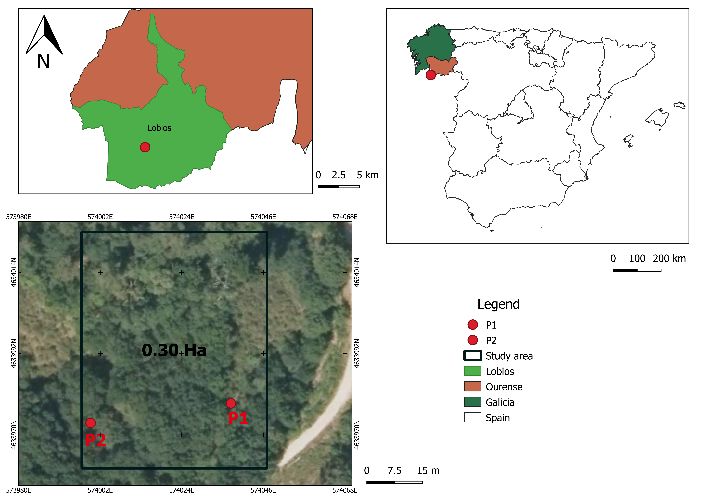
The International Archives of the Photogrammetry, Remote Sensing and Spatial Information Sciences, Volume XLIII-B3-2021
                                                XXIV ISPRS Congress (2021 edition)

classification criterion in Prometheus is the type and height of    To estimate the tree points in the study area, a CHM derived
the propagating element, divided into three well differentiated     from LiDAR was used to detect Individual Tree Crowns (ITC).
groups: grass, shrub, and tree. The information extracted from      Two pre-processing steps prepare a watershed segmentation
the LiDAR data corresponds with the number of points in each        approach: (1) Gaussian filtering and (2) inversion of CHM. The
generated interval. Moreover, the percentage of vegetation          processing toolbox type smooth with gaussian filtering of Orfeo
points of the study area have been estimated. An algorithm          toolbox was used to stablish a circular structuring element of a
developed in Python language performs the automated process.        radius of 2 pixels. In the next step, the smoothed CHM was
Once the percentage of points in each band was calculated the       inverted by the toolbox invert grid of SAGA. Finally, the
next step was the application of the classification conditions      watershed segmentation toolbox of SAGA was used to calculate
carried out to found out the fuel model. Figure 4 shows the fuel    the geolocation of points. The height of each individual tree was
models according to Prometheus in the study area.                   estimated through the CHM using the QGIS point sampling
                                                                    plugin.

       Figure 4. Fuels classified by Prometheus model.
                                                                               Figure 6. Individual tree crowns detection
The next step consists of testing the parameters calculated for
study plots with the field data. Besides, the study was
complemented with the calculation of the following parameters:                   3. RESULTS AND DISCUSSION
biomass estimation and number of trees detected in the study
                                                                    Table 1 shows the results obtained in LiDAR data processing
area. The biomass value was estimated by GIS analysis. A
                                                                    and the ground truth between plot 1 and plot 2 in the study area.
digital vegetation model is a normalized surface model in which
the ground values are subtracted. A Canopy Height Model
                                                                                               PLOT 1                PLOT 2
(CHM) was computed as a difference between Digital Surface
Model (DSM) and Digital Terrain Model (DTM). At first, DTM                                        Ground                Ground
                                                                                           LiDAR                 LiDAR
                                                                                                    truth                 truth
is created from the ground returns and a DSM from the first
                                                                     HERBACEOUS
returns. They were calculated from the tool las2dem selecting                                 21         17            21     26.5
the last pulse, which represents the ground, and the first pulse     HEIGHT (CM)
representing other elevated features on the ground as trees.        SHRUB HEIGHT
                                                                                             165        150            -       57
                                                                         (CM)
CHM was generated containing the information of tree heights.
                                                                      MAXIMUM
To calculate the volume occupied by trees the CHM was                                        9.56       6.0       10.81        8.0
multiplied by the area of each pixel (0.10 m × 0.10 m = 0.01          HEIGHT (M)
m2). The sum of all volumes (m3) in the study area was               % WITHOUT
                                                                                             0.11        0         0.33         0
                                                                         CCF
calculated using a zone statistics tool.
                                                                          %
                                                                     HERBACEOUS              0.03       0.05       0.14        0.9
                                                                         CCF
                                                                     % SHRUB CCF             0.01       0.05        -         0.05
                                                                      FUEL TYPE               5          5         5-6         5

                                                                     Table 1. Comparison results of LiDAR data and ground truth

                                                                    The total height in Plot 1 of study detected by LiDAR data in
                                                                    herbaceous stratum was 21 cm in comparison with the 17 cm of
                                                                    the ground truth collected. The result of LiDAR was 4 cm
                                                                    highest in plot 1, while in plot 2 was the contrary, the total
                                                                    height in herbaceous stratum was 21 cm in comparison with the
                                                                    26.5 cm of the ground truth used. On the one hand, the height
                                                                    shrub detected by LiDAR analyses was 165 cm for shrub in plot
                                                                    1, in comparison with the 150 cm collected in the field. On the
                                                                    other hand, in plot 2 no shrub stratum was detected in the
        Figure 5. CHM of study area in 2019 and 2020                LiDAR analyses, while the ground truth showed a 57 cm
                                                                    present in the plot 2 study. The maximum height parameters

                                               This contribution has been peer-reviewed.
                https://doi.org/10.5194/isprs-archives-XLIII-B3-2021-603-2021 | © Author(s) 2021. CC BY 4.0 License.             606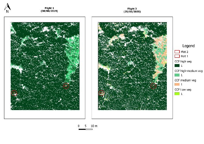
The International Archives of the Photogrammetry, Remote Sensing and Spatial Information Sciences, Volume XLIII-B3-2021
                                                XXIV ISPRS Congress (2021 edition)

showed higher differences between LiDAR data and ground              (medium vegetation: 0.5 m - 2 m), the average height in 2020 is
truth, being the Lidar height calculation higher than the ground     6 cm higher than in 2019. In the group of high shrubs (2 m - 4
truth collected by a vertex instrument. In the plot 1 of study the   m), the average height is similar in both years, showing 6 cm
maximum height detected was of 9.56 m, while in the ground           higher vegetation in 2019 than in 2020, contrary to the high
truth was 6 m. The maximum height detected in plot 2 was             vegetation group (> 4 m), whose results show an increment of
10.81 m while in ground truth was 8 m. There is a                    50 cm in the tree height between the period of 2019 and 2020.
correspondence of approximate 2 m between plots height in            The total average height in the study area was also increased,
both data. Except for herbaceous and shrub height of LiDAR           registering a total of 8.95 m in 2019 and 9.58 m in 2020, so the
data in plot 2, generally the LiDAR data was higher than the         increment of height was of 63 cm.
ground truth data.
                                                                     Figure 8 shows the results of CCF obtained for each stratum. In
The percentage of CCF calculated by LiDAR data processing            all groups is appreciable the decrease of CCF in both years,
showed a lower result than CCF estimated in the field. The           which represents a 5% in tree groups and a 3% in low and
ground truth data showed no percentage without CCF in both           higher shrubs groups. The area without CCF is increased in a
study plots, while LiDAR data results detected a 0.11% of plot       6% in 2020.
1 without CCF and a 0.33% in plot 2. Herbaceous and shrub
CCF calculated by LiDAR data showed a lower percentage than
in ground truth, besides there is no result of shrub CCF in plot 2
of study.

The comparison in the analysis of Prometheus classification
showed the accuracy in the classification of LiDAR height
stratums. Results of vegetation classification detected a fuel
type 5 in both plots. Moreover, areas with presence of fuel type
6 were detected in plot 2.

These differences between LiDAR data and ground truth could
result from the buffer analysis around the plots. The exact same
portion of plots has not been extracted, so there is an
overestimation in the results. As a result, the most highlighted
error detected was in the height shrubs with an absolute error of          Figure 8. Fraction canopy cover in both study years.
15 cm in plot 1 and 57 cm in plot 2, while the highest accuracy
in results was in the CCF shrubs with an absolute error of 0.04
% in plot 1 and 0.05 % in both 2.                                    The analysis of fuel types showed lower cover area in year 2020
                                                                     than in 2019 with exception of fuel type 6, which covers a total
Focused on the analysis of structural forest changes in whole        of 10 m2 more in 2020. The fuel type 6 covered 178 m2 lower in
area of study there was analyzed the average height of each          2020.
stratum. The vegetation was divided in 4 classes and the
following parameters were calculated: CCF, biomass, number           The results obtained for biomass parameter shows an increment
of individual trees, area occupied for each fuel type and the        with a result of 27,644 m3 for 2019 and 28,227 m3 for 2020. A
average height. These parameters were analyzed in both years         total of 583 m3 in a study area of 0.30 Ha was increased during
of study. To carry on the study of structural changes the area       the study year.
was divided in cells of 2 x 2 m for an exhaustive analysis.
                                                                     The total number of points which represents the individual trees
Results of average height are shown in Figure 7 in both years of     detection were 834 in 2019 and 573 in 2020, 771 of which are
recorder LiDAR data in this study, 2019 and 2020.                    trees in 2019 and 531 in 2020. In conclusion 0.23% of trees
                                                                     increased in the study area during a year.

                                                                                          4. CONCLUSIONS

                                                                     The present study showed a promising approach to characterize,
                                                                     classify, and temporally evaluate forest fuels on a woodland
                                                                     area. Some limitations, however, should be pointed out. The
                                                                     difference obtained between the ground truth in comparison
                                                                     with LiDAR processing is based on the different location of the
                                                                     square plots. This is caused by establishment of the buffer
                                                                     influence area on the average coordinates. Moreover, the
                                                                     difference could be related with the accuracy specification up to
                                                                     1cm in horizontal and 2.5 cm in vertical positioning of the UAV
                                                                     data recorder.
               Figure 7. Average height stratums
                                                                     CCF results for year 2019 were higher than CCF in 2020. This
In the first vegetation group, herbaceous group (low vegetation:     could be caused by the high number of points. Point cloud of
0.15 m - 0.5 m) is 0.03 m lower in 2020 than in 2019, although       first flight contains a total of 1,074,390 points, while a total of
show similar values in both years. With respect to low shrubs        705,852 points come from the point cloud of second flight
                                                                     (2020).

                                                This contribution has been peer-reviewed.
                 https://doi.org/10.5194/isprs-archives-XLIII-B3-2021-603-2021 | © Author(s) 2021. CC BY 4.0 License.               607
The International Archives of the Photogrammetry, Remote Sensing and Spatial Information Sciences, Volume XLIII-B3-2021
XXIV ISPRS Congress (2021 edition)
The point cloud classification has been compared according to Meteorology 250. Elsevier: 181–191.
Prometheus system, obtaining the same results than in field Franklin, Janet. 2010. Mapping Species Distributions: Spatial
measures, so it can conclude the accuracy of the method. The Inference and Prediction. Cambridge University Press.
maximum error associated in LiDAR processing was in Franklin, Steven E. 2001. Remote Sensing for Sustainable
herbaceous and shrubs stratums, and it could be originated by Forest Management. CRC press.
the penetration limitation of LiDAR caused by dense canopy Fu, Xiaoyao, Zhengnan Zhang, Lin Cao, Nicholas C Coops,
cover in the study area. Tristan R H Goodbody, Hao Liu, Xin Shen, and
Xiangqian Wu. 2021. “Assessment of Approaches for
Results of statistical analysis of point cloud show the possibility Monitoring Forest Structure Dynamics Using Bi-
to use UAV LiDAR data to characterize changes in the structure Temporal Digital Aerial Photogrammetry Point Clouds.”
of vegetation since the changes in a year also were significant. Remote Sensing of Environment 255. Elsevier: 112300.
Guo, Xuan, Nicholas C Coops, Piotr Tompalski, Scott E
The results of this study have special interest for forest Nielsen, Christopher W Bater, and J John Stadt. 2017.
management. To generate the spatial characteristics of “Regional Mapping of Vegetation Structure for
vegetation in an automated way undoubtedly provides new Biodiversity Monitoring Using Airborne Lidar Data.”
possibilities in modelling the structure of vegetation, including Ecological Informatics 38. Elsevier: 50–61.
defining biometric features and biomass, which determines the Isenburg, Martin. 2012. “LAStools-Efficient Tools for LiDAR
developmental stage of trees and shrubs forming the succession Processing.” Available at: Http: Http://Www. Cs. Unc.
process. Edu/~ Isenburg/Lastools/[Accessed October 9, 2012].
LaRue, Elizabeth A, Brady S Hardiman, Jessica M Elliott, and
Songlin Fei. 2019. “Structural Diversity as a Predictor of
ACKNOWLEDGEMENTS Ecosystem Function.” Environmental Research Letters
14 (11). IOP Publishing: 114011.
A.N. wants to thank University of Vigo through the grant LaRue, Elizabeth A, Franklin W Wagner, Songlin Fei, Jeff W
Axudas Predoutorais para a formación de Doutores 2019 (grant Atkins, Robert T Fahey, Christopher M Gough, and
number 00VI 131H 6410211) and “Expenses were partially Brady S Hardiman. 2020. “Compatibility of Aerial and
covered by the Travel Award sponsored by the open access Terrestrial LiDAR for Quantifying Forest Structural
journal Sensors published by MDPI.” J.M.-S. wants to thank Diversity.” Remote Sensing 12 (9). Multidisciplinary
Ministerio de Ciencia, Innovación y Universidades for the Digital Publishing Institute: 1407.
support through the project PID2019-108816RB-I00. “Phoenix LiDAR Systems.” https://www.phoenixlidar.com/.
QGIS. 2018. “QGIS SOFTWARE.”
https://www.qgis.org/en/site/.
REFERENCES Szostak, Marta. 2020. “Automated Land Cover Change
Detection and Forest Succession Monitoring Using
Albini, Frank A. 1976. Estimating Wildfire Behavior and LiDAR Point Clouds and GIS Analyses.” Geosciences 10
Effects. Vol. 30. Department of Agriculture, Forest (8). Multidisciplinary Digital Publishing Institute: 321.
Service, Intermountain Forest and Range …. Timilsina, Nilesh, Wendell P Cropper, Francisco J Escobedo,
Atkins, Jeff W, Gil Bohrer, Robert T Fahey, Brady S Hardiman, and Joanna M Tucker Lima. 2013. “Predicting
Timothy H Morin, Atticus E L Stovall, Naupaka Understory Species Richness from Stand and
Zimmerman, and Christopher M Gough. 2018. Management Characteristics Using Regression Trees.”
“Quantifying Vegetation and Canopy Structural Forests 4 (1). Multidisciplinary Digital Publishing
Complexity from Terrestrial Li DAR Data Using the Institute: 122–136.
Forestr r Package.” Methods in Ecology and Evolution 9 Van Rossum, Guido. 2007. “Python Programming Language.”
(10). Wiley Online Library: 2057–2066. In USENIX Annual Technical Conference, 41:36.
Bakx, Tristan R M, Zsófia Koma, Arie C Seijmonsbergen, and
W Daniel Kissling. 2019. “Use and Categorization of
Light Detection and Ranging Vegetation Metrics in
Avian Diversity and Species Distribution Research.”
Diversity and Distributions 25 (7). Wiley Online Library:
1045–1059.
Dandois, Jonathan P, Marc Olano, and Erle C Ellis. 2015.
“Optimal Altitude, Overlap, and Weather Conditions for
Computer Vision UAV Estimates of Forest Structure.”
Remote Sensing 7 (10). Multidisciplinary Digital
Publishing Institute: 13895–13920.
Fahey, Robert T, Jeff W Atkins, Christopher M Gough, Brady S
Hardiman, Lucas E Nave, Jason M Tallant, Knute J
Nadehoffer, Christoph Vogel, Cynthia M Scheuermann,
and Ellen Stuart‐Haëntjens. 2019. “Defining a Spectrum
of Integrative Trait‐based Vegetation Canopy Structural
Types.” Ecology Letters 22 (12). Wiley Online Library:
2049–2059.
Fotis, Alex T, Timothy H Morin, Robert T Fahey, Brady S
Hardiman, Gil Bohrer, and Peter S Curtis. 2018. “Forest
Structure in Space and Time: Biotic and Abiotic
Determinants of Canopy Complexity and Their Effects
on Net Primary Productivity.” Agricultural and Forest
This contribution has been peer-reviewed.
https://doi.org/10.5194/isprs-archives-XLIII-B3-2021-603-2021 | © Author(s) 2021. CC BY 4.0 License. 608You can also read