GENERATING REALISTIC STOCK MARKET ORDER STREAMS - OpenReview
←
→
Page content transcription
If your browser does not render page correctly, please read the page content below
Under review as a conference paper at ICLR 2019

G ENERATING R EALISTIC S TOCK M ARKET O RDER
S TREAMS
 Anonymous authors
 Paper under double-blind review

                                            A BSTRACT

         We propose an approach to generate realistic and high-fidelity stock market data
         based on generative adversarial networks. We model the order stream as a stochas-
         tic process with finite history dependence, and employ a conditional Wasserstein
         GAN to capture history dependence of orders in a stock market. We test our ap-
         proach with actual market and synthetic data on a number of different statistics,
         and find the generated data to be close to real data.

1   I NTRODUCTION

Financial markets are among the most well-studied and closely watched complex multiagent sys-
tems in existence. Well-functioning financial markets are critical to the operation of a complex
global economy, and small changes in the efficiency or stability of such markets can have enormous
ramifications. Accurate modeling of financial markets can support improved design and regulation
of these critical institutions. There is a vast literature on financial market modeling, though still a
large gap between the state-of-art and the ideal. Analytic approaches provide insight through highly
stylized model forms. Agent-based models accommodate greater dynamic complexity, and are often
able to reproduce “stylized facts” of real-world markets (LeBaron, 2006). Currently lacking, how-
ever, is a simulation capable of producing market data at high fidelity and high realism. Our aim
is to develop such a model, to support a range of market design and analysis problems. This work
provides a first step, learning a high-fidelity generator from real stock market data streams.
Our main contribution is an approach to produce stock market data that is close to real market data,
using a Wasserstein generative adversarial network (WGAN) (Arjovsky et al., 2017). There are
many challenges that we overcome as part of this contribution. The first is how to represent a stream
of stock market orders as data that can be used in a WGAN. Towards this end, we assume the stock
market data stream to arise from a stochastic process with finite (but long) memory dependence. The
stochastic process view also makes precise the conditional distribution that the generator is learning
as well the joint distribution that the critic of the WGAN distinguishes by estimating the earth-mover
distance.
The second main challenge is the design of the network architecture. We choose a conditional
WGAN to capture the history dependence of the stochastic process, with both the generator and
critic conditional on history of orders and the time of day. A single LSTM layer is used to summarize
the history succinctly. The internal architecture of both the generator and critic uses a standard
convolutional structure. The generator outputs the next stock market order as well as how this order
changes the active orders in the market. Part of the generator output, which updates the active market
orders, is produced using a pre-trained network to approximate the deterministic buy and sell order
matching in the stock market.
Finally, we experiment with synthetic and real market data. The synthetic data is produced using
a stock market simulator that has been used in several agent-based financial studies. The real data
was obtained from OneMarketData, a financial data provider and publisher of the OneTick database
product. We evaluate the generated data using various statistics such as the distribution of price and
quantity of orders, inter-arrival times of orders, and the best bid and best ask evolution over time. We
find the generated data matches the corresponding statistics in real data (simulated or actual stock
market) closely.

                                                   1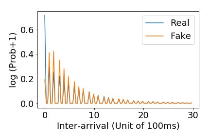
Under review as a conference paper at ICLR 2019

                     Figure 1: Visual representation and evolution of a limit order book.

2       R ELATED W ORK AND BACKGROUND
WGAN is a popular and well-known variant of GANs (Goodfellow et al., 2014). Most prior work
on generation of sequences using GANs has been in the domain of text generation (Press et al.,
2017; Zhang et al., 2017). However, since the space of word representations is not continuous, the
semantics change with nearby word representation, and given a lack of agreement on the metrics
for measuring goodness of sentences, producing good quality text using GANs is still an active
area of research. Stock market data does not suffer from this representation problem but the history
dependence for stock markets can be much longer than for text generation. In a sequence of recent
papers, Xiao et al. (2017; 2018) have introduced GAN-based methods for generating point processes.
The proposed methods generate the time for when the next event will occur. The authors have also
explored the use of these techniques to generate the time for transaction events in stock markets.
Our problem is richer as we aim to generate the actual limit orders including time, order type, price,
and quantity information.
Deep neural networks and machine learning techniques have been used on financial data mostly for
prediction of transaction price (Hiransha et al., 2018; Bao et al., 2017; Qian, 2017) and for prediction
of actual returns (Abe & Nakayama, 2018). As stated, our goal is not market prediction per se, but
rather market modeling. Whereas the problems of learning to predict and generate may overlap
(e.g., both aim to capture regularity in the domain), the evaluation criteria and end product are quite
distinct.
The stock market is a venue where equities or stocks of publicly held companies are traded.
Nearly all stock markets follow the continuous double auction (CDA) mechanism (Friedman, 1993).
Traders submit bids, or limit orders, specifying the maximum price at which they would be willing
to buy a specified quantity of a security, or the minimum price at which they would be willing to
sell a quantity.1 The order book is a store that maintains the set of active orders: those submitted
but not yet transacted or canceled. CDAs are continuous in the sense that when a new order matches
an existing (incumbent) order in the order book, the market clears immediately and the trade is ex-
ecuted at the price of the incumbent order—which is then removed from the order book. Orders
may be submitted at any time, and a buy order matches and transacts with a sell order when the
limits of both parties can be mutually satisfied. For example, as shown in Figure 1 if a limit buy
order with price $10.01 and quantity 100 arrives and the order book has the best offered sell price at
$10.01 with quantity 100 then the arriving order matches an incumbent exactly. However, the next
buy order does not match any sell, and the following sell order partially matches what is then the
best buy in the order book.
The limit order book maintains the current active orders in the market (or the state of the market),
which can be described in terms of the quantity offered to buy or sell across the range of price
levels. Each order arrival changes the market state, recorded as an update to the order book. After
processing any arrived order every buy price level is higher than all sell price levels, and the best bid
    1
        Hence, the CDA is often referred to as a limit-order market in the finance literature (Abergel et al., 2016).

                                                           2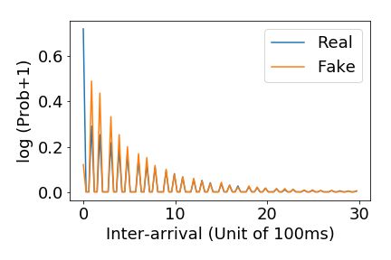
Under review as a conference paper at ICLR 2019

refers to the lowest buy price level and the best ask refers to the highest sell price level. See Figure 1
for an illustration. The order book is often approximated by few (e.g., ten) price levels above the
best bid and ten price levels below the best ask; as these prices are typically the ones that dictate
the transactions in the market. There are various kinds of traders in a stock market, ranging from
individual investors to large investing firms. Thus, there is a wide variation in the nature of orders
submitted for a security. We aim to generate orders for a security in aggregate (not per agent) that
is close to the aggregate orders generated in a real market. We focus on generating orders and do
not attempt to generate transactions in the stock market. This is justified as the CDA mechanism is
deterministic and transactions can be determined exactly given a stream of orders.

3     S TOCK -GAN
3.1   S TOCK M ARKET O RDERS AS A S TOCHASTIC P ROCESS

We model stock market orders as a stochastic process. Recall that a stochastic process is a collection
of random variables indexed by a set of numbers. We view the stock market orders for a given chunk
of time of day ∆t as a collection of vector valued random variable {xi }i∈N indexed by the limit order
sequence number in N = {1, . . . , n}. The components of the random vector xi include the time
interval di , type of order ti , limit order price pi , limit order quantity qi , and the best bid ai and best
ask bi . The time interval di specifies the difference in time between the current order i and previous
order i − 1 (in precision of milliseconds); the range of di is finite. The type of order can be buy, sell,
cancel buy, or cancel sell (represented in two bits). The price and quantity are restricted to lie within
finite bounds. The price range is discretized in units of US cents and the quantity range is discretized
in units of the equity (non-negative integers). The best bid and best ask are limit orders themselves
and are specified by price and quantity. Observe that we assume the stochastic process depends on
the discrete time of day ∆t, which we will make explicit in the next paragraph. We divide the time
in a day into 25 equal intervals and ∆t refers to the index of the interval. A visual representation of
xi is shown in Figure 2(a).
Following the terminology prevalent for stochastic processes, the above process is discrete time
and discrete space (note that discrete time in this terminology here refers to the discreteness of
the index set N ). We assume a finite history dependence of the current output xi , that is, P (xi |
xi−1 , . . . , ∆t) = P (xi | xi−1 , . . . , xi−m , ∆t). Such dependence is justified by the observation that
recent orders mostly determine the transactions and transaction price in the market as orders that
have been in the market for long either get transacted or canceled. Further, the best bid and best
ask serves as an (approximate) sufficient statistic for events beyond the history length m. While this
process is not a Markov chain, it forms what is known as a higher order Markov chain, which implies
that the process given by yi = (xi , . . . , xi−m+1 ) is a Markov chain for any given time interval
∆t. We assume that this chain formed by yi has a stationary distribution (i.e., it is irreducible and
positive recurrent). A Markov chain is a stationary stochastic process if it starts with its stationary
distribution. After some initial mixing time, the Markov chain does reach its stationary distribution,
thus, we assume that the process is stationary by throwing away some initial data for the day. Also,
for the jumps across two time intervals ∆t, we assume the change in stationary distribution is small
and hence the mixing happens very quickly. A stationary process means that P (xi , . . . , xi−m+1 |
∆t) has the same distribution for any i. In practice we do not know m. However, we can assume a
larger history length k + 1 > m, and then it is straightforward to check that yt = (xi , . . . , xi−k ) is
a Markov chain and the claims above hold with m − 1 replaced by k. We choose k = 20.

3.2   WGAN A RCHITECTURE AND W ORKING

Given the above stochastic process view of the problem, we design a conditional WGAN with a
recurrent architecture to learn the real conditional distribution Pr (xi | xi−1 , . . . , xi−k , ∆t). We use
the subscript r to refer to real distributions and the subscript g to refer to generated distributions.
The real data x1 , x2 , . . . is a realization of the stochastic process. It is worth noting that even
though P (xi , . . . , xi−k | ∆t) has the same distribution for any i, the realized real data sequence
xi , . . . xi−k is correlated with any overlapping sequnce xi+k0 , . . . xi−k+k0 for k ≥ k 0 ≥ −k. Our
data points for training (stated in detail in the next paragraph) are sequences xi , . . . xi−k , and to
ensure independence in a batch we make sure that the sequences chosen in a batch are sufficiently
far apart.

                                                      3
Under review as a conference paper at ICLR 2019
(a) xi (b) Generator (c) Critic
Figure 2: Stock-GAN architecture
Architecture: The architecture is shown in Figure 2. Our proposed WGAN is conditional (Mirza
& Osindero, 2014) with both the generator and critic conditioned on a k length history and the time
interval ∆t. The history is condensed to one vector using a single LSTM layer. This vector and
some uniform noise is fed to a fully connected layer layer followed by a convolutional structure.
The generator outputs the next xi (realization of xi ) and the critic outputs one real number. Note
that when training both generator and critic are fed history from real data, but when the generator
executes after training it is fed its own generated data as history. As stated earlier, the generator
output includes the best bid and ask. As the best bid and ask can be inferred deterministically from
the current order and the previous best bid and ask (for most orders), we use another neural network
(with frozen weights during GAN training) to output the best bid and ask. We call this the CDA
network. The CDA network is trained separately using a standard MSE loss (see Appendix C).
Critic details: When fed real data, the critic can be seen as a function cw of si =
(xi , . . . , xi−k , ∆t), where w are the weights of the critic network. As argued earlier, samples in
a batch that are chosen from real data
1
Pmthat are spaced at least k apart are i.i.d. samples of Pr . Then
for m samples fed to the critic, m i=1 cw (si ) estimates Es∼Pr (cw (s)). When fed generated data
(with the ten Pm price levels determined from the output order and previous ten levels), by similar rea-
1
soning m i=1 cw (si ) estimates Es∼Pg (cw (s)) when the samples are sufficiently apart (recall that
the history is always real data). Thus, the critic computes the Wasserstein distance between the joint
distributions Pr (xi , . . . , xi−k , ∆t) and Pg (xi , . . . , xi−k , ∆t). Further, we use a gradient penalty
term in the loss function for the critic instead of clipping weights as proposed in the original WGAN
paper (Arjovsky et al., 2017) because of the better performance as revealed in prior work (Gulrajani
et al., 2017).
Generator details: The generator learns the conditional distribution Pg (xi | xi−1 , . . . , xi−k , ∆t).
Along with the real history, the generator represents the distribution Pg (xi , . . . , xi−k , ∆t) = Pg (xi |
xi−1 , . . . , xi−k , ∆t)Pr (xi−1 , . . . , xi−k , ∆t).
The loss functions used is the standard WGAN loss function with a gradient penalty term (Gulrajani
et al., 2017). The critic is trained 100 times in each iteration and as already stated, the notable part
in constructing the training data is that for each mini-batch the sequence of orders chosen (including
history) is far away from any other sequence in that mini-batch (see Appendix C for code snippets).
4 E XPERIMENTAL R ESULTS
We apply and evaluate Stock-GAN on two types of data sets composed of orders from an agent-
based market simulator and from a real stock market, respectively. We describe each data set in
detail and then compare key metrics and distributions of our generated orders with ground truth
orders from the agent-based simulator and real stock markets.
4Under review as a conference paper at ICLR 2019
4.1 S YNTHETIC AND R EAL DATA
Synthetic data: We first evaluate Stock-GAN on synthetic orders generated from an agent-based
market simulator. Previously adopted to study a variety of issues in financial markets (e.g., market
making and manipulation), the simulator captures stylized facts of the complex financial market
with specified stochastic processes and distributions (Wellman & Wah, 2017). We briefly describe
the market simulator below.
In the simulation, the market operates over a finite time horizon. Agents enter and reenter the market
according to a Poisson process with an arrival rate of 0.005. On each arrival these traders submit a
limit order to the market (replacing their previous order, if any), indicating the price at which they
are willing to buy or sell a single unit of the security. The market environment is populated by
32 traders, representing investors. Each investor has an individual valuation for the security made
up of private and common components. The common component is represented by a fundamental
value, which can be viewed as the intrinsic value of the security. This fundamental value varies over
time according to a mean-reverting stochastic process. The private component of value captures
the preference contribution of the individual agent’s reason for trading this security at the current
time (e.g., investment, liquidity, diversification). The private valuations are drawn from a specified
distribution at the start of a simulation. The common and private components are effectively added
together to determine each agents valuation of the security. Agents accrue private value on each
transaction, and at the end of the trading horizon evaluate their accumulated inventory on the basis
of a prediction of the end-time fundamental. Given the market mechanism and valuation model
for the simulation, investors pursue their trading objectives by executing a trading strategy in that
environment. A popular trading strategy we adopt in the simulator is the zero-intelligence (ZI)
strategy (Farmer et al., 2005). The ZI trader shades its bid from its current valuation of the stock by
a random offset. We use about 300,000 orders generated by the simulator as our synthetic data. The
price output by the simulator is normalized to lie in the interval [−1, 1].
Real data: We obtained real limit-order streams from OneMarketData, who provided access for
our research to their OneTick database for selected time periods and securities. The provided data
streams comprise order submissions and cancellations across multiple exchanges at millisecond
granularity. In experiments, we evaluate in the performance of Stock-GAN on two securities: a small
capitalization stock, Patriot National (PN), and a large capitalization stock, Alphabet Inc (GOOG).
The two stocks differ in several key aspects, including investment sector, market activity intensity,
price range, liquidity etc., and thus their order patterns represent distinct dynamic processes. By
training Stock-GAN with historical data for individual stocks, we can generate limit-order streams
that capture key characteristics of each.
Relative to our simulated agent-based market, the real market limit orders tend be very noisy includ-
ing many orders at extreme prices far from the range where transactions occur. Since our interest
is primarily on behavior that can affect market outcomes, we focus on limit orders in the relevant
range near the best bid and ask. Specifically, in a preprocessing step, we eliminate limit orders that
never appear within ten levels of the best bid and ask prices. In the experiment reported here, we
use historical real market data of PN during one trading day in August 2016, and GOOG during one
trading day in August 2017. After preprocessing, the PN daily order stream has about 20,000 orders
and GOOG has about 230,000.
4.2 E VALUATION S TATISTICS
We generate a number of orders equal to the number of real orders used to train the WGAN. We
evaluate our generated order stream in comparison to real data using the following statistics:
1. Price. Distribution over price for the day’s limit orders, by order type.
2. Quantity. Distribution over quantity for the day’s limit orders, by order type.
3. Inter-arrival time. Distribution over inter-arrival durations for the day’s limit orders, by
order type.
4. Intensity evolution. Number of orders for consecutive 1000-second chunks of time.
5. Best bid/ask evolution. Changes in the best bid and ask over time as new orders arrive.
5Under review as a conference paper at ICLR 2019
(a) Simulated price distribution (b) Simulated quantity distribution (c) Simulated inter-arrival dist.
(d) PN price distribution (e) PN quantity distribution (f) PN inter-arrival dist.
(g) GOOG price distribution (h) GOOG quantity distribution (i) GOOG inter-arrival dist.
Figure 3: Simulated, PN, and GOOG submitted buy-order statistics.
A note on cancellation: In our generation process, cancellation type orders are not contingent on
the order book. We use a heuristic which is to match the generated cancellation order to the closest
priced order in the book. Cancellations that are too far from any existing order to be a plausible
match are ignored.
4.3 R ESULTS
In describing our results, “real” refers to simulated or actual stock market data and “fake” refers to
generated data. Figure 3 presents statistics on buy orders for the three cases when the real data is
simulated, PN, or GOOG. For simulated data, the price and inter-arrival distribution matches the real
distribution quite closely. The quantity for the simulated data is always one, which is also trivially
captured in the generated data. For PN and GOOG, the quantity distribution misses out on some
peaks but gets most of the peaks in the real distribution. The inter-arrival time distribution matches
quite closely (note that the axis has been scaled for inter-arrival time to highlight the peaks and show
the full range of time). The price distribution matches closely for GOOG, but is slightly off for PN,
which could be due to the low amount of data for PN.
Figure 4 presents statistics on sell orders for the three cases when the real data is simulated, PN,
or GOOG. The results for sell orders are quite similar to buy orders. Results for cancellations are
included in the appendix.
Figure 5 presents order intensity as a function of time (number of orders in every chunk of 1000
secs normalized by max number) for the simulated, PN, and GOOG markets. As in the graphs for
other statistics, generated WGAN results are compared with the measured intensities in the real data.
The intensities show similar trends, though for the real markets there is significant variation. The
6Under review as a conference paper at ICLR 2019
(a) Simulated price distribution (b) Simulated quantity distribution (c) Simulated inter-arrival dist.
(d) PN price distribution (e) PN quantity distribution (f) PN inter-arrival dist.
(g) GOOG price distribution (h) GOOG quantity distribution (i) GOOG inter-arrival dist.
Figure 4: Simulated, PN, and GOOG submitted sell-order statistics.
(a) Simulated (b) PN (c) GOOG
Figure 5: Intensity of market activities that include all types of orders across the trading period.
differences are particularly large for PN, likely due to the relatively smaller magnitude of trading
volume for that stock.
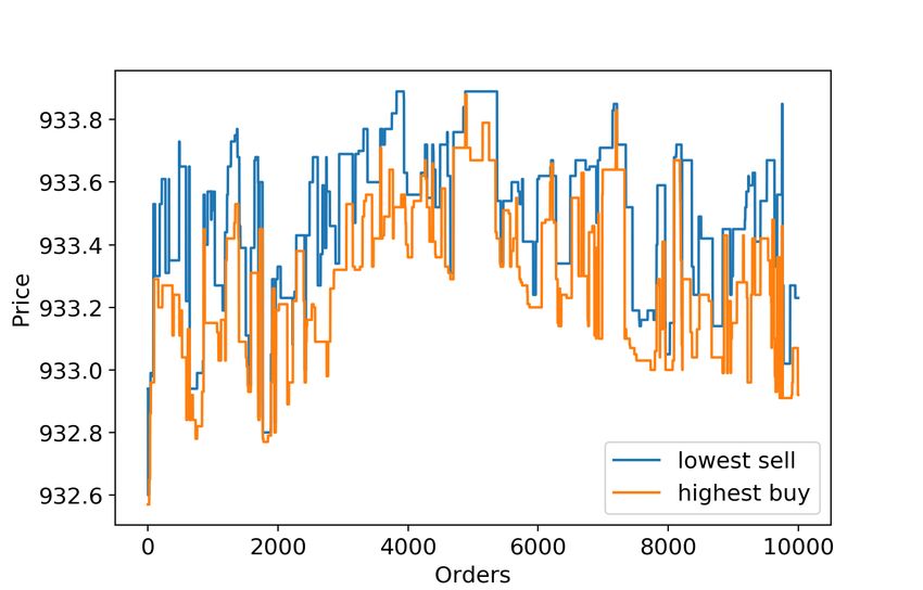
In Figure 6, we show the change in best buy/ask as a function of time for the simulated, PN, and
GOOG markets. The generated results looks similar to real data in range and variation over time for
simulated data. The similarity to real best bid/ask is better for GOOG than PN, which could possibly
be due to more data available for GOOG.
Quantitative measures: The figures till now show that the price distribution appears like a normal
distribution and the inter-arrival time appears like a geometric distribution (geometric is discrete
version of exponential). We fit these standard distributions to the real price and inter-arrival distribu-
tion and compare the total variation (TV) distance between the real and fitted vs real and generated
7Under review as a conference paper at ICLR 2019
(a) Simulated best bids and asks. (b) Real PN best bids and asks. (c) Real GOOG best bids and asks.
(d) Fake best bids and asks. (e) Fake PN best bids and asks. (f) Fake GOOG best bids and asks.
Figure 6: Best bid and ask evolution across order book state changes.
Simulated PN GOOG
TV distance between Price IA Price IA Price IA
Real and Fitted (buy) 0.4910 0.8457 1.3449 1.0571 1.0573 1.2953
Real and Generated (buy) 0.7439 0.2847 1.6828 0.2373 1.0614 0.3631
Real and Fitted (sell) 0.4968 0.8516 1.5453 0.9912 1.0546 1.3869
Real and Generated (sell) 0.8246 0.2025 1.4813 0.2477 1.1572 0.3286
Table 1: TV distance comparisons between fitted and generated distribution. IA means inter-arrival.
distributions. The quantity distribution does not appear like any standard distribution, hence we do
not evaluate it by fitting. The results in Table 1 show that the generated price distribution is almost as
close to the real one as the fitted price distribution. The generated inter-arrival distribution is much
closer to the real one than the fitted price distribution. A point to note is that the actual price and
quantity is a stochastic process with dependence on history, thus, the fitted distributions will not be
helpful in generating the correct intensities or best bid and best ask evolution.
A note on architectural choices: Various parts of our architecture were developed iteratively to
improve the results that we obtained in a previous iteration. The input of ∆t to the generator and
critic is critical to get the time trend in the intensity for the GOOG stock. The CDA network and the
best bid and ask in history was added to improve the results for best bid/ask variation over time.
Comparision with baseline: We also implemented a variational recurrent generative network but
found its performance to be worse than our approach (shown in Appendix B).
5 C ONCLUSION
Our results reveal that GANs can be used to simulate a stock market. While our results are promis-
ing, there are open issues that provide for further research material. One experimental aspect is to
try different size of the network in the WGAN, possibly dependent on the data size of the given
stock and testing with many different variety of stocks. Another open research issue is to output
cancellations in a more intelligent manner than the heuristic approach we use now. Overall, our
work provides fertile ground for future research at the intersection of deep learning and finance.
8Under review as a conference paper at ICLR 2019
R EFERENCES
Masaya Abe and Hideki Nakayama. Deep learning for forecasting stock returns in the cross-section.
In Pacific-Asia Conference on Knowledge Discovery and Data Mining, pp. 273–284, 2018.
Frédéric Abergel, Anana Marouane, Anirban Chakraborti, Aymen Jedidi, and Ioane Muni Toke.
Limit Order Books. Cambridge University Press, 2016.
Martin Arjovsky, Soumith Chintala, and Léon Bottou. Wasserstein generative adversarial networks.
In 34th International Conference on Machine Learning, pp. 214–223, 2017.
Wei Bao, Jun Yue, and Yulei Rao. A deep learning framework for financial time series using stacked
autoencoders and long-short term memory. PLOS One, 12(7):e0180944, 2017.
Junyoung Chung, Kyle Kastner, Laurent Dinh, Kratarth Goel, Aaron C Courville, and Yoshua Ben-
gio. A recurrent latent variable model for sequential data. In Advances in neural information
processing systems, pp. 2980–2988, 2015.
J. Doyne Farmer, Paolo Patelli, and Ilija I. Zovko. The predictive power of zero intelligence in
financial markets. Proceedings of the National Academy of Sciences, 102:2254–2259, 2005.
Daniel Friedman. The double auction market institution: A survey. The Double Auction Market
Institutions, Theories and Evidence, Addison Wesley, 1993.
Ian Goodfellow, Jean Pouget-Abadie, Mehdi Mirza, Bing Xu, David Warde-Farley, Sherjil Ozair,
Aaron Courville, and Yoshua Bengio. Generative adversarial nets. In Advances in neural infor-
mation processing systems, pp. 2672–2680, 2014.
Ishaan Gulrajani, Faruk Ahmed, Martin Arjovsky, Vincent Dumoulin, and Aaron C Courville. Im-
proved training of Wasserstein GANs. In Advances in Neural Information Processing Systems,
pp. 5767–5777, 2017.
M. Hiransha, E. A. Gopalakrishnan, Vijay Krishna Menon, and K. P. Soman. NSE stock market
prediction using deep-learning models. Procedia Computer Science, 132:1351 – 1362, 2018.
International Conference on Computational Intelligence and Data Science.
Blake LeBaron. Agent-based computational finance. In Leigh Tesfatsion and Kenneth L. Judd
(eds.), Handbook of Computational Economics. Elsevier, 2006.
Mehdi Mirza and Simon Osindero. Conditional generative adversarial nets. arXiv preprint
arXiv:1411.1784, 2014.
Ofir Press, Amir Bar, Ben Bogin, Jonathan Berant, and Lior Wolf. Language generation with re-
current generative adversarial networks without pre-training. arXiv preprint arXiv:1706.01399,
2017.
Xin-Yao Qian. Financial series prediction: Comparison between precision of time series models
and machine learning methods. arXiv preprint arXiv:1706.00948, 2017.
Michael P. Wellman and Elaine Wah. Strategic agent-based modeling of financial markets. Russell
Sage Foundation Journal of the Social Sciences, 3(1):104–119, 2017.
Shuai Xiao, Mehrdad Farajtabar, Xiaojing Ye, Junchi Yan, Le Song, and Hongyuan Zha. Wasserstein
learning of deep generative point process models. In Advances in Neural Information Processing
Systems, pp. 3247–3257, 2017.
Shuai Xiao, Hongteng Xu, Junchi Yan, Mehrdad Farajtabar, Xiaokang Yang, Le Song, and
Hongyuan Zha. Learning conditional generative models for temporal point processes. In 32nd
AAAI Conference on Artificial Intelligence, 2018.
Yizhe Zhang, Zhe Gan, Kai Fan, Zhi Chen, Ricardo Henao, Dinghan Shen, and Lawrence Carin.
Adversarial feature matching for text generation. arXiv preprint arXiv:1706.03850, 2017.
9Under review as a conference paper at ICLR 2019
A A DDITIONAL R ESULTS
Below we show results for buy order cancellation and sell order cancellation using the exact same
measures as for the buy and sell orders in the main paper. The results also are similar to buy or sell
results earlier.
(a) Simulated cancel buy order price.(b) Simulated cancel buy order (c) Simulated cancel buy order inter-
quantity. arrival.
(d) PN cancel buy order price. (e) PN cancel buy order quantity. (f) PN cancel buy order inter-arrival.
(g) GOOG cancel buy order price. (h) GOOG cancel buy order quan- (i) GOOG cancel buy order inter-
tity. arrival.
Figure 7: Simulated, PN, and GOOG cancelled buy orders statistics.
10Under review as a conference paper at ICLR 2019
(a) Simulated cancel sell order price.(b) Simulated cancel sell order (c) Simulated cancel sell order inter-
quantity. arrival.
(d) PN cancel sell order price. (e) PN cancel sell order quantity. (f) PN cancel sell order inter-arrival.
(g) GOOG cancel sell order price. (h) GOOG cancel sell order quan- (i) GOOG cancel sell order inter-
tity. arrival.
Figure 8: Simulated, PN and GOOG sell cancel orders.
11Under review as a conference paper at ICLR 2019
(a) GOOG price distribution (b) GOOG quantity distribution (c) GOOG inter-arrival dist.
Figure 9: Simulated, PN, and GOOG submitted buy-order statistics using recurrent VAE.
(a) GOOG intensity plot
Figure 10: Intensity of market activities for GOOG using recurrent VAE.
B VARIATIONAL RECURRENT NEURAL NETWORK
We use the variational recurrent network as another baseline generative model. The architec-
ture is exactly same as the work Chung et al. (2015). We used the code available at https:
//github.com/phreeza/tensorflow-vrnn, but modified it. Our modification was to en-
able not forcing the output to be Gaussian as done in Chung et al. (2015), as those produced much
worse results. Instead, we use a MSE loss. We also modified the input size, etc. to make the neural
network structure compatible with our problem. The exact change to the code changing the loss
function is shown below:
kl loss = tf kl gaussgauss ( enc mu , enc sigma , prior mu , prior sigma )
# we replace the maximium likelihood loss with the mse loss below
mse loss = tf. losses . mean squared error (y, dec rho )
return tf. reduce mean ( kl loss + mse loss )
The results in Figure 9 for GOOG buy order only and in Figure 10 for all types of GOOG orders
shows that the entropy of the output is high (when comparing price and inter-arrival distributions)
and the performance is worse than our GAN. In particular, the generated (fake) price distribution is
wider than the real one (or the one generated by the GAN). The generated inter-arrival distribution
is almost uniform over the discrete time points and not concentrated at 0. The quantity distribution
matches the real one, somewhat similarly like our GAN approach, but it generates some negative
values unlike our GAN approach (which could be discarded). The intensity distribution is also
somewhat close to the real intensity. The results are similar for other types of orders.
12Under review as a conference paper at ICLR 2019
C C ODE S NIPPETS
Here we present codes snippets that show the architecture of the GAN. First, we start with the CDA
network that is trained independently with MSE loss:
input his = Input ( shape =(8 ,))
G = Sequential (name=’discriminator ’)
G.add( Dense (256∗3 , input dim =8))
G.add( BatchNormalization ())
G.add( Activation (’relu ’))
G.add( Reshape ((16 , 16, 3)))
G.add( Conv2D (128 ,(3 ,3) , padding =’same ’))
G.add( BatchNormalization ())
G.add( Activation (’relu ’))
G.add( Conv2D (64 , (3 ,3) , padding =’same ’))
G.add( BatchNormalization ())
G.add( Activation (’relu ’))
G.add( Conv2D (32 ,(3 ,3) , padding =’same ’))
G.add( BatchNormalization ())
G.add( Activation (’relu ’))
G.add( Flatten ())
G.add( Dense (4))
output vec = G( input his )
self.net = Model ( inputs = input his , outputs = output vec )
optimizer = Adam (0.0001)
self.net. compile ( optimizer =optimizer , loss=’ mean squared error ’)
self.net. summary ()
Input LSTM structure for both Generator and Critic are shown below
# ########## Input for both Generator and Critic #######################
# history orders of shape (self. historyLength , self. orderLength )
history = Input ( shape =( self. historyLength , self. orderLength ), \
name=’ history full ’)
# current time slot: Integer , from 0 to 23
history input = Input ( shape =(1 ,) , name=’ history time ’)
# noise input of shape (self. noiseLength )
noise input 1 = Input ( shape =( self. noiseLength ,), name=’ noise input 1 ’)
# Real order of shape (( self. mini batch size ,self. orderLength )
truth input = Input ( shape =( self. mini batch size ,\
self. orderLength ,1) , name=’ truth input ’)
# lstm at Generator to extract history orders features
lstm output = LSTM(self. lstm out length )( history )
# lstm at Critic to extract history orders features
lstm output h = LSTM(self. lstm out length ,name=’ lstm critic ’)( history )
# concatenate history features with noise
gen input = Concatenate (axis=−1)([ history input , lstm output , noise input 1 ])
The Generator structure is shown below, which includes the trained CDA network
# ############ Generator ########################
# Input : gen input , shape (self. noiseLength +self. lstm out length + 1)
13Under review as a conference paper at ICLR 2019
# Output : gen output 1 , shape (self. mini batch size ,self. orderLength − 4)
dropout = 0.5
G 1 = Sequential (name=’ generator 1 ’)
G 1 .add( Dense (( self. orderLength −4)∗self. mini batch size ∗100 , \
input dim =self. noiseLength +self. lstm out length + 1))
G 1 .add( BatchNormalization ())
G 1 .add( Activation (’relu ’))
G 1 .add( Reshape (( int(self. mini batch size ), int(self. orderLength − 4), 100)))
G 1 .add( UpSampling2D ())
G 1 .add( Dropout ( dropout ))
G 1 .add( UpSampling2D ())
G 1 .add( Conv2DTranspose (32 , 32, padding =’same ’))
G 1 .add( BatchNormalization ())
G 1 .add( Activation (’relu ’))
G 1 .add( Conv2DTranspose (16 ,32 , padding =’same ’))
G 1 .add( BatchNormalization ())
G 1 .add( Activation (’relu ’))
G 1 .add( Conv2DTranspose (8, 32, padding =’same ’))
G 1 .add( BatchNormalization ())
G 1 .add( Activation (’relu ’))
G 1 .add( MaxPooling2D ((2 ,2)))
G 1 .add( Conv2DTranspose (1, 32, padding =’same ’))
G 1 .add( Activation (’tanh ’))
G 1 .add( MaxPooling2D ((2 ,2)))
gen output 1 = G 1 ( gen input )
#CDA network ( train offline )
# Input : cda input , shape (self. mini batch size , 8)
# Output : gen output 2 , shape (self. mini batch size , 4)
G 2 = Sequential (name=’ orderbook gen ’)
G 2 .add( Dense (256∗3 , input dim =8))
G 2 .add( BatchNormalization ())
G 2 .add( Activation (’relu ’))
G 2 .add( Reshape ((16 , 16, 3)))
G 2 .add( Conv2D (128 ,(3 ,3) , padding =’same ’))
G 2 .add( BatchNormalization ())
G 2 .add( Activation (’relu ’))
G 2 .add( Conv2D (64 , (3 ,3) , padding =’same ’))
G 2 .add( BatchNormalization ())
G 2 .add( Activation (’relu ’))
G 2 .add( Conv2D (32 ,(3 ,3) , padding =’same ’))
G 2 .add( BatchNormalization ())
G 2 .add( Activation (’relu ’))
G 2 .add( Flatten ())
G 2 .add( Dense (4))
# extract the last best bid/ask from history as the history of CDA
orderbook history = Lambda ( lambda x: x[:,−1,5:], output shape =(4 ,))( history )
# gen output 1 is output of generator
gen output reshaped = Reshape (( self. orderLength −4,))( gen output 1 )
# remove time as it is not needed for CDA network
gen output without time = \
Lambda ( lambda x: x[: ,1:] , output shape =(4 ,))( gen output reshaped )
cda input = Concatenate (axis =1)([ gen output without time , orderbook history ])
gen output 2 = G 2 ( cda input )
# Output of Generator , shape (self. mini batch size , self. orderLength ) concatentated
# with output of the CDA network to get final output
14Under review as a conference paper at ICLR 2019
gen output = Concatenate (axis =2)([ gen output 1 ,\
Reshape (( self. mini batch size , 4, 1))( generator output 2 )])
The structure of the critic is shown below
# ############ Critic ##################
# Input of Critic , merge history input , lstm output h and gen output / truth input
discriminator input fake = ( Concatenate (axis =2)\
([ Reshape ((1 , 1 ,1))( history input ), \
Reshape ((1 , self. lstm out length ,1))( lstm output h ), gen output ]))
discriminator input truth = Concatenate (axis =2)\
([ Reshape ((1 , 1 ,1))( history input ), \
Reshape ((1 , self. lstm out length ,1))( lstm output h ), truth input ])
#random−weighted average of real and generated samples − following
# Improved WGAN work
averaged samples = RandomWeightedAverage ()\
([ discriminator input fake , discriminator input truth ])
# Critic
# Input : discriminator input fake / discriminator input truth
# Ouput : score
D = Sequential (name=’discriminator ’)
D.add( Conv2D (512 ,(3 ,3) , padding =’same ’, input shape =( self. mini batch size , \
self. orderLength +self. lstm out length +1 ,1)))
D.add( Activation (’relu ’))
D.add( Conv2D (256 , (3 ,3) , padding =’same ’))
D.add( Activation (’relu ’))
D.add( Conv2D (128 ,(3 ,3) , padding =’same ’))
D.add( Activation (’relu ’))
D.add( Flatten ())
D.add( Dense (1))
#self.D = D
discriminator output fake = D( discriminator input fake )
discriminator output truth = D( discriminator input truth )
averaged samples output = D( averaged samples )
#Def gradient penalty loss
partial gp loss = partial (self. gradient penalty loss ,
averaged samples = averaged samples ,
gradient penalty weight =1)
partial gp loss . n a m e = ’ gradient penalty ’
The full model
# ############## Model Definition ################
# Generator model
# Input : [ history input ,history , noise input 1 ]
# Output : gen output
self.gen = Model ( inputs =[ history input ,history , noise input 1 ], outputs = gen output )
# Model Truth :
self. model truth = Model ( inputs =[ history input ,history , noise input 1 , truth input ] ,\
outputs =[ discriminator output fake , discriminator output truth ,\
averaged samples output ])
# Model Fake:
self. model fake = Model ( inputs =[ history input ,history , noise input 1 ] ,\
outputs = discriminator output fake )
# Optimizer
optimizer = Adam (0.0001 , beta 1 =0.5 , beta 2 =0.9)
15Under review as a conference paper at ICLR 2019
# Compile Models
# Generator
self.gen. compile ( optimizer =optimizer , loss=’ binary crossentropy ’)
self.gen. summary ()
# Model Truth − Generator is not trainable here
for layer in self. model truth . layers :
layer . trainable = False
self. model truth . get layer (name=’discriminator ’). trainable = True
self. model truth . get layer (name=’ lstm critic ’). trainable = True
self. model truth . compile ( optimizer =optimizer , \
loss =[ self. w loss ,self. w loss , partial gp loss ])
# Model Fake − critic is not trainable here
for layer in self. model fake . layers :
layer . trainable = True
self. model fake . get layer (name=’discriminator ’). trainable = False
self. model fake . get layer (name=’ lstm critic ’). trainable = False
self. model fake . compile ( optimizer =optimizer , loss=self. w loss )
# print summary
self. model fake . summary ()
self. model truth . summary ()
16You can also read