Grasping asymmetric information in market impacts
←
→
Page content transcription
If your browser does not render page correctly, please read the page content below
Grasping asymmetric information in market impacts
                                                   Shanshan Wang1 , Sebastian Neusüß2 and Thomas Guhr1
arXiv:1710.07959v2 [q-fin.TR] 22 Apr 2019

                                                   1
                                                     Fakultät für Physik, Universität Duisburg–Essen, Lotharstraße 1, 47048 Duisburg,
                                                   Germany
                                                   2
                                                     Deutsche Börse AG, Frankfurt, Germany
                                                   E-mail: shanshan.wang@uni-due.de

                                                   23 April 2019

                                                   Abstract. The price impact for a single trade is estimated by the immediate response
                                                   on an event time scale, i.e., the immediate change of midpoint prices before and
                                                   after a trade. We work out the price impacts across a correlated financial market.
                                                   We quantify the asymmetries of the distributions and of the market structures of
                                                   cross-impacts, and find that the impacts across the market are asymmetric and non-
                                                   random. Using spectral statistics and Shannon entropy, we visualize the asymmetric
                                                   information in price impacts. Also, we introduce an entropy of impacts to estimate
                                                   the randomness between stocks. We show that the useful information is encoded in
                                                   the impacts corresponding to small entropy. The stocks with large number of trades
                                                   are more likely to impact others, while the less traded stocks have higher probability
                                                   to be impacted by others.

                                                   PACS numbers: 89.65.Gh 89.75.Fb 05.10.Gg
                                                   Keywords: market impact, asymmetric information, eigenvalue spectra,
                                                   entropy, network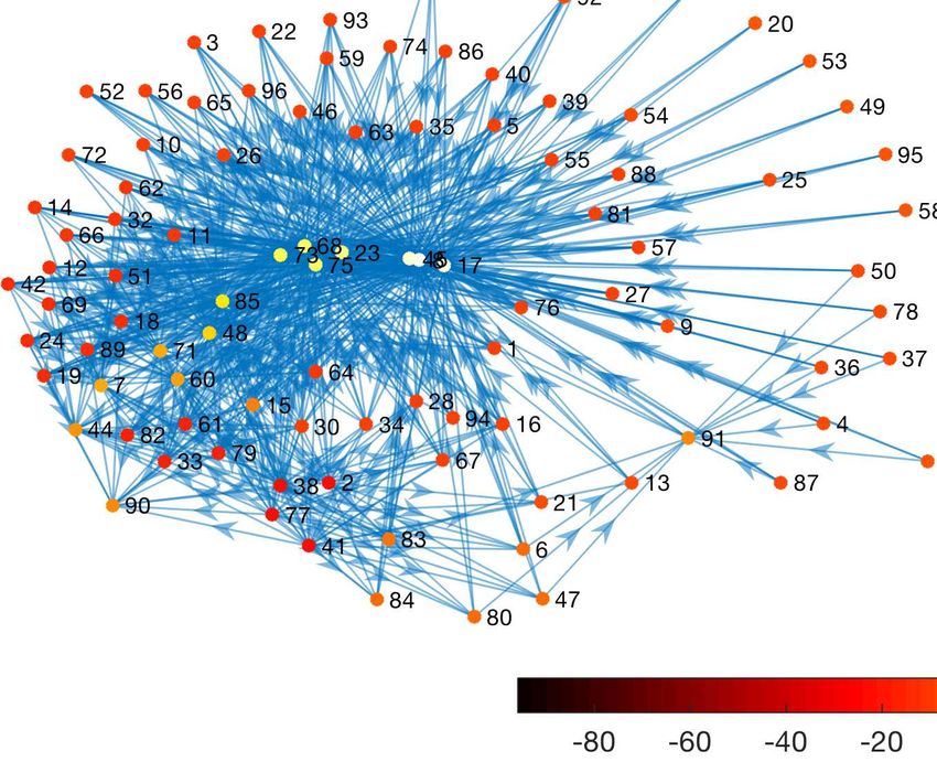
Grasping asymmetric information in market impacts                                             2

Contents

1 Introduction                                                                                2
2 Data description                                                                            3
  2.1 Data set . . . . . . . . . . . . . . . . . . . . . . . . . .     . . . . . . . . . .    3
  2.2 Order reconstruction . . . . . . . . . . . . . . . . . . .       . . . . . . . . . .    4
  2.3 Data processing . . . . . . . . . . . . . . . . . . . . . .      . . . . . . . . . .    5
3 Asymmetry of price impacts                                                                  5
  3.1 Measurement of impacts . . . . . . . . . . . . . . . . .         . . . . . . . . . .    6
  3.2 Asymmetry of distributions . . . . . . . . . . . . . . .         . . . . . . . . . .    9
  3.3 Asymmetry of the market structure . . . . . . . . . . .          . . . . . . . . . .   10
4 Eigenvalue spectra of asymmetric market structures                                         11
5 Entropy of asymmetric market structures                                                    14
  5.1 Entropy of eigenvalue spectra . . . . . . . . . . . . . .        . . . . . . . . . .   14
  5.2 Entropy of price impacts . . . . . . . . . . . . . . . . .       . . . . . . . . . .   15
  5.3 Networks of price impacts . . . . . . . . . . . . . . . .        . . . . . . . . . .   18
6 Conclusions                                                                                20
Acknowledgments                                                                              21
Appendix A Trading data                                                                      22

1. Introduction

In the last two decades, the microstructure of financial markets has attracted ever
more attention. An enormous amount of available transaction data makes quantitative
analyses possible. Since the 1960s when Mandelbrot found the fat-tailed distribution
of cotton prices [1], many stylized facts in the price dynamics [2–4] were identified. In
particular, the price change caused by trades exhibits non-Markovian features [5–8],
which drive the market to temporarily deviate from an efficient state [7]. The average
price change due to a trade is referred to as price impact [9]. The price impact in
single stocks is more likely to induce an extra cost of trading, termed liquidity cost [10].
To reduce such costs, traders split orders, which partially leads to the long-memory
correlation in the order flow [5, 11]. The impact from a large split order is termed market
impact [12, 13]. These findings have considerable practical and theoretical importance.
      Recently, empirical studies [7, 8, 14] disclosed that there are also price impacts across
stocks. To avoid confusion, the impact in single stocks is named self-impact and the
impact between stocks is named cross-impact. Different from the costs arising from the
self-impact, the extra costs [15–17] caused by the cross-impact are often ignored in the
optimal execution of orders [18–23]. From a “no-dynamic-arbitrage” perspective, the
cross-impact should be symmetric [15]. However, the empirical cross-impact from asset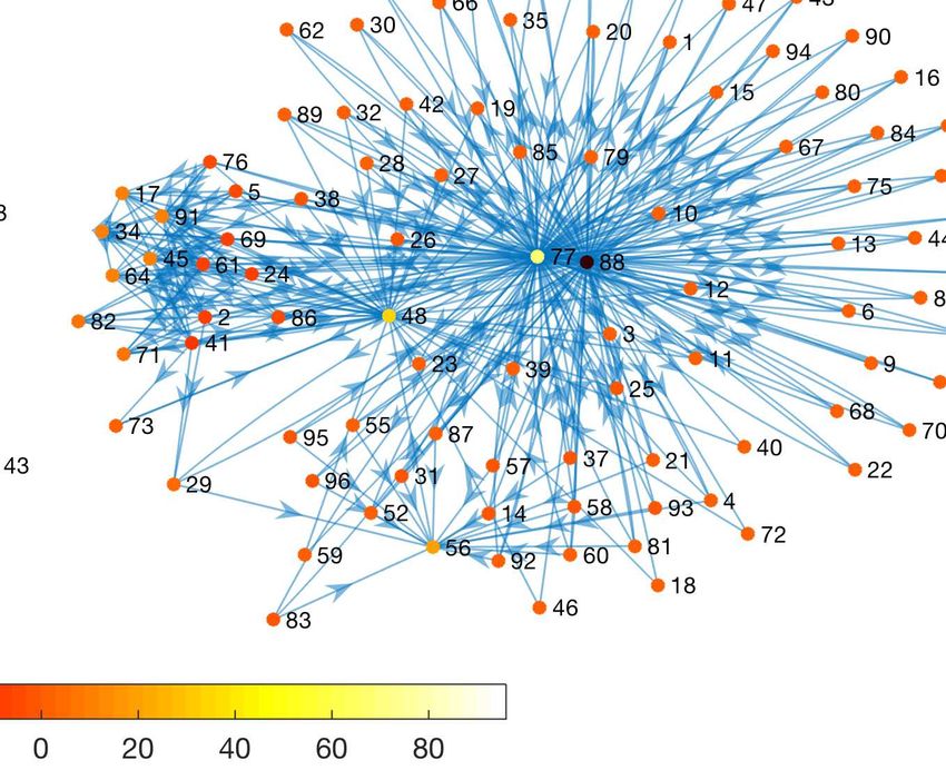
Grasping asymmetric information in market impacts                                         3

i to asset j is not equal to the one from asset j to asset i [15]. Regardless of the bid-ask
spread, the asymmetry of cross-impacts implies that, first, the information distributed
in the market is asymmetric, and second, arbitrage is possible if using special strategies.
     The self-impact has been more extensively studied and estimated than the cross-
impact, partially due to the difficulties in the empirical estimation. Without a proper
estimation, biases may be present either in the cross-impact or in the costs arising
from it. We empirically analyzed the cross-response and the cross-impact on a physical
time scale [7, 8, 24] with a one-second resolution. In their study, Benzaquen et al.
used time intervals of five minutes [14]. Both choices of time scales have advantages
and limitations. Schneider et al. therefore use the combined trade time [15]. In the
present study, we focus on the immediate responses. More precisely, we analyze how
a subsequent quote change in one stock is caused by a trade in another stock. In
this sense, we use an event time scale. The immediate response helps to conveniently
estimate the impact without a time lag. This impact leads to an increase in transaction
costs immediately and obviously compared to the impact with a time lag. If we were
able to grasp the important information of the immediate impact, we could use this
information in trading strategies of multiple stocks for reducing transaction costs, or
in risk management for setting an alert line. We analyze these impacts across the
whole, correlated market and identify and quantify the asymmetry of the information.
Furthermore, the Shannon entropy [25] helps us to assess the degree of randomness for
the impacts and to extract other useful features.
     The paper is organized as follows. In Sect. 2, we discuss the data. In Sect. 3, we
measure the asymmetry of impacts across the market. In Sect. 4, we analyze the spectral
statistics of asymmetric impacts. To estimate the degree of randomness, we introduce
the Shannon entropy and construct directional networks of impacts with given entropy
matrices in Sect. 5. The conclusions are presented in Sect. 6.

2. Data description

We introduce the data set in Sect. 2.1, and explain the order reconstruction from the
historical data in Sect. 2.2. We then describe the procedure of data processing in
Sect. 2.3.

2.1. Data set
We use the TotalView-ITCH data set, where 96 stocks from NASDAQ stock market,
in NASDAQ 100 index are listed. The TotalView-ITCH data set contains the order
flow data with all the events, for instance, the submissions, cancellations and executions
of limit orders. It has a resolution of one millisecond that is much higher than the
resolution of one second in the Trade and Quote (TAQ) data set [26]. Hence, plenty of
order flow data in each trading day are recorded in the TotalView-ITCH data set. For
each stock, we take into account the intraday data of five trading days from March 7th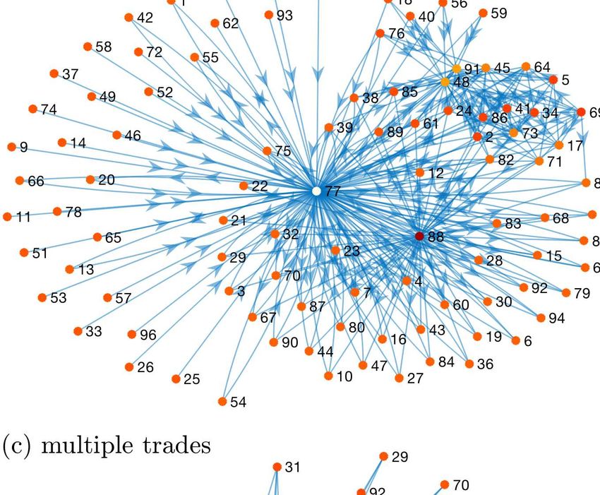
Grasping asymmetric information in market impacts                                         4

to March 11th of 2016, obtained from Tradingphysics [27]. Unlike the TAQ data set, the
TotalView-ITCH data set does not provide the information of quotes and trades directly.
To gain these information, reconstruction of the order book is required. In addition,
the trade and quote data used in our study are restricted to the intraday trading time
from 9:40 to 15:50 EST. The stocks and the average daily number of trades during this
period are listed in A.

2.2. Order reconstruction
The basic idea for the order reconstruction is to simulate the trading of the stock market
with the historical order flow data while organizing the orders into the order book. The
historical order flow data can be found in the TotalView-ITCH data set, which records
all limit orders with the message for processing. The limit orders enter the order book
time-ordered and wait for a better trade price. They are distinguished from another
type of orders, i.e., the market orders, which are executed immediately at the present
available price.
      To begin with, we download the order flow data from the TotalView-ITCH data
set and inject the limit orders into an order pool. The order pool is a place where all
the limit orders are gathered and processed according to the message carried by each
order. The message includes eight types, submission to buy (B), submission to sell (S),
cancellation in part (C), cancellation in full (D), execution in part (E), execution in
full (F), bulk volumes for cross events (X) and executions of non-display orders (T).
We ignore the types X and T, because of the difficulty to identify the trade types and
because they are sparse compared to the other types. In the order pool, a submitted limit
order is placed at a price level by the principle of primary price priority and secondary
time priority. The submitted order will raise the available volume at that price level.
However, if a cancellation or an execution is released to an order, the volume at the
price level at which the order is placed is reduced in part or in full. To trace an order
with different messages, we follow the unique ID given to an order when it enters the
order pool. Orders with smaller ID numbers are submitted earlier. If the volume at
a certain price level vanishes completely, the order ID and the corresponding price are
deleted from the order pool. Therefore, a message issued to an order will change either
the price or the volume. To make such information visible, all prices and corresponding
volumes are listed in the order book. It is updated to a new arrangement by a new
message, such that the minimal (maximal) price to sell (buy), i.e., the best ask (bid),
with the lowest ID number is always listed at the beginning of the ask (bid).
      We say there is a new best quote if either the best ask price, the best bid price, the
best ask volume or the best bid volume is changed. In this way, we are able to filter the
best quote data. We also notice that an execution of a limit order matches a trade of
a market order. The trade type of the limit order is opposite to the one of the market
order, but the trade price as well as the traded volume for the two orders coincide.
Using the message of limit orders, we derive the trade information and obtain the trade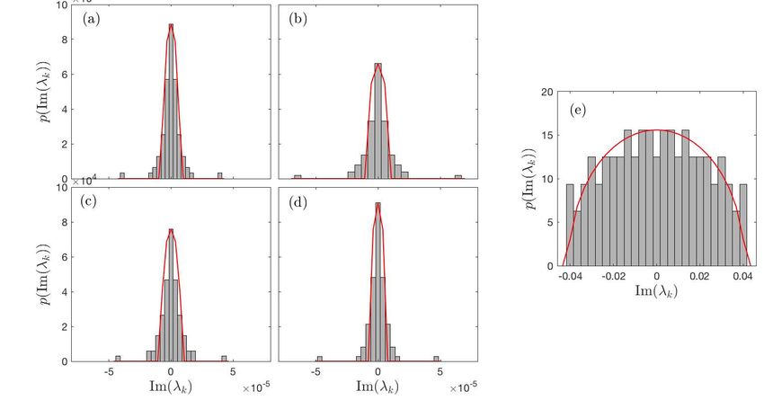
Grasping asymmetric information in market impacts                                                5

                                       ∆mi                    ∆mi
           stock i                                                         ti   a quote
                       previous                following
                                                                                a buy trade
           stock j                                                              a sell trade
                                                                           tj

                                     a case of               a case of
                                  multiple trades          single trades

               Figure 1. Examples for the cases of multiple trades and single trades, ti and tj are
               the event times of stocks i and j, respectively, ∆mi is the price change between the
               previous and the following quotes of stock i for a given trade of stock j.

data. The data can be distinguished on the level of one millisecond. To facilitate the
data processing in the following, we only consider events with a single trade in a given
millisecond. If there are more than one trade in one-millisecond interval, we exclude all
these trades in that interval. The average proportion of excluded trades to total trades
is 10.44%.

2.3. Data processing
To estimate the immediate change in the quotes due to a trade, we track each trade. If
a trade of stock j occurs at time t (measured on the event scale), the last quote of stock
i in time t − 1 is treated as the previous quote of that trade and accordingly the first
quote of stock i in time t+1 as the following quote. If the latter quote is generated while
a trade of stock i occurring, this trade is regarded as being triggered by the preceding
trade of stock j at time t. Thus, the quote change of stock i can be attributed to the
trade of stock j.
     In fact, the previous and following quotes are not always directly before and after
a trade. There may be several time stamps before or after the trade, such that multiple
trades of stock j may share the same previous quote as well as the following quote. We
name them cases of multiple trades, shown in Fig. 1. Hence, a single trade is not enough
to cause the price change of another stock until several trades occur. Still, there is a
part of trades that does not share the previous and following quotes with others. We
name them cases of single trades, see Fig. 1. We estimate the average probabilities for
the trades belonging to the cases of multiple trades and of single trades as 0.35 and
0.65, respectively. Despite the lower proportion compared to the case of single trades,
the case of multiple trades contains a part of the daily transactions. Thus, we take both
cases into account.

3. Asymmetry of price impacts

We employ a price response function to measure the impacts across stocks and to
distinguish four types of responses in Sect. 3.1. For the whole market, we measure
Grasping asymmetric information in market impacts 6
the asymmetry of distributions of responses in Sect. 3.2 and also quantify the structural
asymmetry of response matrices in Sect. 3.3.
3.1. Measurement of impacts
The response function in Refs. [7, 8] measures how a buy or sell order at time t influences
on average the price at a later time t + τ . The physical time scale was chosen since the
trades in different stocks are not synchronous. Here, we rather use a response function
on an event time scale, as we are interested in the immediate responses. The time lag τ
is restricted to one such that the price response quantifies the price impact of a single
trade. We define it as
D E
(f ) (p)
Rij = log mi (tj ) − log mi (tj ) εj (tj ) (1)
tj
(p)
for the price change of stock i caused by a trade of stock j. Here, mi (tj ) is the midpoint
(f )
price of stock i previous to the trade of stock j at its event time tj and mi (tj ) is the
midpoint price of stock i following that trade. The trade sign εj (tj ) of stock j is defined
either as +1 for a buy or as −1 for a sell market order. On the event time scale,
zero trade signs are absent. The sign of each trade can be obtained empirically from
TotalView-ITCH data set. The symbol h· · ·itj indicates an average over the event time
tj .
It is worthwhile relating the response (1) to the model set up in Ref. [24]. The
response Rij (τ ) for a stock pair (i, j) with a time lag τ is modelled by
(s) (c)
Rij (τ ) = Rij (τ ) + Rij (τ ) , (2)
(s)
where Rij (τ ) is related to self-impacts Gii (·) and cross-correlators of trade signs Θij (·)
and Θji (·)
(s)
X
Rij (τ ) = Gii (t + τ − t′ ) hfi (vi (t′ ))it Θij (t′ − t)
t≤t′Grasping asymmetric information in market impacts 7
Let Gij be the price impact of a single trade between stocks i and j, which contains the
effects due to the trade volumes of stock j, and let Θij be the correlator of trade signs
without any time lag. Equation (5) then is transformed into
X
Rij = Gii Θij + Gij Θjj = Gin Θnj . (6)
n=i,j
Here, only the stocks i and j (i 6= j) are considered. For the whole market, the price
change of stock i can be regarded as the result of price impacts from all stocks n,
n = 1, · · · , N. Consequently, the price response for a single trade between stocks i and
j is expressed as
N
X
Rij = Gin Θnj . (7)
n=1
Let G and Θ be the N × N impact and correlator matrices with entries Gin and Θnj ,
respectively. The immediate responses for the whole market then can be formulated as
a matrix product, where the N × N response matrix R with entries Rij reads,
R = GΘ . (8)
We mention that for i = j in Eq. (7), self-impacts prevail over cross-impacts, so that
Rii approximates to Gii Θii = Gii where Θii = 1. For i 6= j, Eq. (7) approximates to
Rij = Gii Θij + Gij , as the cross-terms without the self-impact or the sign self-correlator
are too trivial. In our study, the self-impact Gii from a trade of stock i might occur at
the moment of updating the following quote or might be absent between the previous
and the following quotes. If we treat this trade as being triggered by the preceding trade
of a different stock j, the potential self-impact is incorporated into the cross-impact and
the term Gii Θij vanishes. From this perspective, the price cross-response Rij directly
measures the cross-impact Gij .
By performing different averages, we distinguish the price responses to all trades
Rij |at , to single trades Rij |st and to multiple trades Rij |mt , respectively. Since every trade
in this study is classified either as the case of single trades or as the case of multiple
trades, the averaging over all trades treats the two cases on equal footing. However, the
occurrence of the two cases is never exactly the same for every stock pair. Let wij be
the ratio of the case of single trades to all trades for a stock pair (i, j). We define a
linearly interpolating weighted price response with wij as a weight factor
Rij = wij Rij + (1 − wij )Rij . (9)
wt st mt
Thus, the frequent occurrence of either case will largely affect the weighted response. R
is the N × N response matrix for all pairs of stocks (i, j), where in our case N = 96. In
the response matrix, the diagonal elements are the self-responses, and the off-diagonal
elements are the cross-responses. We work out the empirical response matrices R for the
cases of all trades, single trades, multiple trades and weighted trades, shown in Fig. 2.
As seen, the market responds strongly to the case of single trades but much weaker to
the case of multiple trades. In between are the case of all trades and the weighted case.Grasping asymmetric information in market impacts 8
20
40
10 -6
60 0.01
6
20
0.005
80 4
40
0
2
60
-0.005
0
20 80 -0.01
-2
40 20 40 60 80
60
80
20 40 60 80 20 40 60 80
Figure 2. Market response matrices R in (a) case of all trades, (b) case of single
trades, (c) case of multiple trades, (d) case of weighted trades, and (e) random case.
Table 1. Measurements of asymmetries
All Single Multiple Weighted
Quantities Measurements Random
trades trades trades trades
Mode/right shift (×10−6 ) 1.965 2.710 0.217 2.234 84.500
off Mean (×10 )−6
1.873 3.348 0.793 2.473 26.923
p(Rij )
Median (×10−6 ) 1.775 3.168 0.508 2.354 21.304
Skewness 1.585 1.461 1.893 1.587 -0.018
hΛ(R)i Overall asymmetry 0.360 0.334 0.628 0.317 0.716
H(Im(λ)) Shannon entropy 2.018 1.884 2.120 1.816 3.189
Table 2. Fit parameters of stable distributions
Responses Cases α β γ (×10−6 ) µ0 (×10−6 )
All trades 1.749 0.512 0.748 1.725
Single trades 1.737 0.496 1.230 3.107
Cross-responses
Multiple trades 1.246 0.663 0.480 0.425
Weighted trades 1.792 0.607 0.915 2.298
Self- Single trades 1.493 1 28.798 116.119
responses
Cross- Random 1.999 -1 2208.170 31.333
responsesGrasping asymmetric information in market impacts 9
10 5
7
6
5
4
3
2
1
0
-5 0 5 10 15
10 -6
10000 120
100
8000
80
6000
60
4000
40
2000 20
0 0
2 4 6 8 10 -0.01 -0.005 0 0.005 0.01
10 -4
off
Figure 3. (a) The probability distributions p(Rij ) of price cross-responses to all, to
single, to multiple and to weighted trades, respectively; (b) the probability distribution
diag off
p(Rij ) of price self-responses to single trades; (c) the probability distribution p(Rij |r )
of the off-diagonal elements in the random response matrix R|r . All distributions are
fitted by stable distributions, shown with solid lines.
For comparison, we also consider a random response matrix R|r ,
1
R|r = A sgn(B T ) , (10)
L
where A and B are uncorrelated N × L random matrices with zero mean and unit
variance, L is the length of a time series. The sign function sgn(·) is used to obtain
random signs from a series of random numbers, hence, sgn(B T ) is the L × N matrix of
the signs of B T . The superscript T indicates the adjoint. Different from the other cases,
the random response matrix R|r in Fig. 2 (e) displays a uniform distribution without
any striking feature.
3.2. Asymmetry of distributions
To quantify the response structure of the whole market, we work out the probability
distributions for the four types of responses, see Fig. 3. The cross-responses are the
off-diagonal elements of the response matrix R and the self-responses are the diagonal
elements. The distribution for the off-diagonal elements of the random response matrixGrasping asymmetric information in market impacts 10
R|r is shown in Fig. 3 as well. The modes, means, medians and skewness for the
distributions of cross-responses are listed in Table 1. Each non-random empirical
distribution is shifted to the right of the vertical axis at zero. This asymmetry reveals an
imbalance of positive and negative responses. It implies that a buy (sell) of one stock is
more likely to move up (down) the price of another stock. Although the cross-response
to single trades has the largest right shift of 2.71 × 10⁻⁶ among the four types, it is very
weak compared to the self-response with a shift of 1.23 × 10⁻⁴.
We fit all empirical distributions with stable distributions, a class of probability
distributions modelling skewness and heavy tails [28]. Stable distributions p(x) of a
random variable x are best specified by their characteristic function
Z+∞
ϕ(κ) = exp(iκx)p(x)dx , (11)
−∞
which have the form [28]
h i
exp −γ α |κ|α 1 + iβsgn(κ) tan πα ((γ|κ|)1−α − 1) + iµ0 κ for α 6= 1 ,
2
ϕ(κ) = h i (12)
exp −γ|κ| 1 + iβ 2 sgn(κ) log(γ|κ|) + iµ0 κ for α = 1 .
π
The stability parameter α ∈ (0, 2], strongly affects the tails of the distribution.
When α = 2, the distribution is normal with mean µ0 and variance 2γ 2 , i.e., N (µ0, 2γ 2 ).
When 0 < α < 2, the distribution is non-normal with heavy tails. The shape parameter
β ∈ [−1, 1] describes the skewness of the distribution, which is distinguished from the
classical skewness defined by s = h(x − µ)3 i/σ 3 , where µ is the mean of x and σ is the
standard deviation of x. If β = 0, the distribution is symmetric. If β > 0 (β < 0), the
distribution is right (left) skewed. In addition, the scale parameter γ is restricted to
γ > 0 and the location parameter µ0 is restricted to µ0 ∈ R. The fit parameters of the
proper stable distributions are listed in Table 2. The non-normality and the asymmetry
of the distributions are revealed by the values of α and β. Theses stable distributions
will be used to work out the probabilities for given cross-responses in Sect. 5.2.
3.3. Asymmetry of the market structure
Considering the whole market structure, we further quantify the asymmetry along the
diagonal of each response matrix. For a N × N square matrix X, the asymmetry of X
can be quantified by Λ(X),
||X − X T ||
Λ(X) = , (13)
2||Y ||
where the square matrix Y is defined by Yij = Xij (1 − δij ) and where ||X|| is the
Euclidean norm
v
u N N
uX X
||X|| = t Xij2 . (14)
i=1 j=1Grasping asymmetric information in market impacts 11
The Kronecker delta δij is used to exclude the diagonal elements from X. In particular,
Λ(X) = 0 means that the matrix X is symmetric along the diagonal, while Λ(X) = 1
indicates that X is anti-symmetric along the diagonal. A value of 0 < Λ(X) < 1
arises, when X is asymmetric, where large values of Λ(X) indicate high asymmetry. To
stabilize the measurement, we introduce the following averaging procedure. Let k be an
integer with 1 ≤ k ≤ N and let
Xnn ··· Xn(n+k−1)
Ξ(k|n) = .. .. .. (15)
.
. .
X(n+k−1)n · · · X(n+k−1)(n+k−1)
be a k × k sub-matrix over the diagonal constructed from X, with 1 ≤ n ≤ N − k + 1,
then
NX
−k+1
(k|n) 1
Λ Ξ(k|n) .
hΛ(Ξ )i = (16)
N − k + 1 n=1
is the average asymmetry of all k × k sub-matrices in X. At a fixed dimension k,
the averaging over the index n in Eq. (16) rules out the influence of elements on the
structural asymmetry of X. By a further average
N
1 X
hΛ(X)i = hΛ(Ξ(k|n))i , (17)
N k=1
we obtain the stabilized overall asymmetry of X, as the averaging over the index k
in Eq. (17) eliminate the influence of dimensions on the structural asymmetry of X.
Importantly, the diagonal of the sub-matrices Ξ(k|n) lies on the diagonal of X. Thus,
each Xij is compared with the corresponding Xji .
For our study, the matrix X is the response matrix R. The average asymmetry of
R versus the matrix dimension k is shown in Fig. 4. We find that the asymmetry for a
given response matrix is close to a constant, independent of the dimension k, provided
k is larger than 10 or so. The values of the stabilized overall asymmetries hΛ(R)i are
listed in Table 1. In all cases, symmetry of the response matrices is absent. Hence,
the price impact from stock j to stock i is unequal to the one from stock i to stock j,
i.e., Gij 6= Gji in the model setting. The non-equivalence, for example, in the case of
single trades has a deviation of 33.4%, hinting at a possibility for arbitrage if ignoring
the bid-ask spread. The strong asymmetry in the response structure coincides with the
finding that the empirical cross-impact violates the symmetry condition of “no dynamic
arbitrage” [15].
4. Eigenvalue spectra of asymmetric market structures
Random matrices have been used to analyze the spectrum properties of cross-
correlations of financial data [29–34]. The eigenvalue spectrum of a random correlation
matrix is well known to be given by the Marc̆enko-Pastur distribution [35–37]. These
random correlation matrices are symmetric and the corresponding eigenvalues areGrasping asymmetric information in market impacts 12
0.8
0.7
0.6
0.5
0.4
0.3
0.2
0 10 20 30 40 50 60 70 80 90 100
Figure 4. The asymmetries of response matrices R for four cases and of random
matrix R|r versus the dimension k of matrices.
real. However, for an asymmetric random matrix, the eigenvalues are complex and
a description with the Marc̆enko-Pastur distribution is not appropriate. To analyze
the eigenvalue spectrum of an asymmetric matrix X, we decompose the matrix into a
symmetric part XS and an asymmetric part XA ,
X = XS + XA , (18)
with
XS = (X + X T )/2 and XA = (X − X T )/2 . (19)
Thus, the asymmetry of X is fully accounted for by XA . As XA is anti-symmetric, the
non-zero eigenvalues λk of XA are purely imaginary, given by
XA ψk = λk ψk , (20)
where ψk is the corresponding eigenvector.
The distribution of eigenvalues of random asymmetric matrices was computed by
Sommers et al. [38]. For an ensemble of N × N random asymmetric matrices M, where
the elements Mij are normally distributed with zero mean and correlations
hMij2 i = 1 and hMij Mji i = c (21)Grasping asymmetric information in market impacts 13
for i 6= j and −1 ≤ c ≤ 1, the average density p(ωk ) of eigenvalues ωk = xk + iyk is
given by
(
(πab)−1 , if (xk /a)2 + (yk /b)2 ≤ 1 ,
p(ωk ) = (22)
0, otherwise ,
where a = 1 + c and b = 1 − c. The cases c = 1 and c = 0 correspond to
ensembles of symmetric matrices and fully asymmetric matrices in which Mij and
Mji are independent, respectively. When c = −1, the matrix is anti-symmetric, i.e.,
Mij = −Mji , with non-zero imaginary eigenvalues ±iyk . The projection of p(ωk ) on
the imaginary axis leads to a generalized semicircle law, which describes the probability
density distribution
2
Z
p(yk ) = dxk p(ωk ) = 2 (b2 − yk2)1/2 , |yk | ≤ b . (23)
πb
At the points yk = ±b, the probability densities are equal to zero.
Using Eq. (19), we calculate for all response matrices R the corresponding
asymmetric matrices RA . We compute the eigenvalues of RA and work out the
probability density distributions p(Im(λk )), shown in Fig. 5. The histograms in Fig. 5
are normalized to one. All these distributions are compared with the distributions of
random matrices drawn from Eq. (23). Here, due to the anti-symmetry of RA , c = −1,
such that b = 2. However, the probability densities of Im(λk ) need to be rescaled
to match the normalized histograms. A convenient way is to scale b by a factor of
(πp(0))−1 , because for a normalized histogram, Eq. (23) at the point yk = 0 results in
b = 2/(πp(0)).
As expected, the distribution resulting from Eq. (23) matches well the distribution
for the random case. In contrast, it deviates largely from each of the distributions for the
four types of responses. The differences are significant at the tails of distributions where
the largest imaginary parts of eigenvalues are located. In the previous studies [32, 39],
the largest eigenvalue for cross-correlation matrices are interpreted as the market mode
or collective “response” of the whole market to stimuli, such as economic growth,
interest rate increase, or political events. Because the eigenvector corresponding to the
largest eigenvalue has nonzero components everywhere, the influence represented by the
largest eigenvalue is common to all stocks. In our case, the eigenvectors corresponding
to the largest imaginary parts of eigenvalues are complex. Besides the difficulty
from processing the complex eigenvectors, a lack of relevant data makes it impossible
to identify such market or sector mode. However, the non-random distributions of
eigenvalue spectra suggest that the response matrices contain asymmetric information.
If the market is efficient, the prices should perfectly reflect the information that is
available [40]. As a result, the immediate responses between assets are symmetric [15],
i.e., Rij = Rji and the arbitrage opportunities are absent in the market. However,
the asymmetric information we find reveals that the market is not fully efficient
and arbitrage opportunities can arise. Without such opportunities, there will be no
incentives for traders to acquire information and the price discovery aspect of financialGrasping asymmetric information in market impacts 14
Figure 5. Probability density distributions of imaginary parts of eigenvalues, (a) case
of all trades, (b) case of single trades, (c) case of multiple trades, (d) case of weighted
trades, (e) random case. For comparison, the distributions (23) are displayed as red
lines.
markets will cease to exist [41, 42]. The asymmetric information thus plays a role in
maintaining a natural market ecology, where the possible arbitrage opportunities provide
the motivation for traders to stay in the market.
5. Entropy of asymmetric market structures
We introduce the Shannon entropy [25] to quantify the randomness of eigenvalue spectra
in Sect. 5.1. Making use of the stable distributions, we map the response matrices into
probability matrices and compute the entropy of price impacts in Sect. 5.2. For given
entropy matrices, we construct directional networks for impacts and further explore how
the network evolves with the entropy in Sect. 5.3. Since the price impact for a single
trade is estimated by the immediate response, we use the response for convenience to
represent the price impact in the following.
5.1. Entropy of eigenvalue spectra
We used the eigenvalue spectrum to identify the non-randomness of asymmetric price
impacts, but we have not yet quantified the randomness. To this end, we resort to the
entropy in information theory, also known as the Shannon entropy [25], which is capable
of analyzing the randomness and unpredictability of a system. The Shannon entropy isGrasping asymmetric information in market impacts 15
defined as
n
X
H(Z) = − P (zk ) logξ P (zk ) . (24)
k=1
Here, Z is a discrete random variable with possible values {z1 , · · · , zn }, and P (zk ) is the
probability of the value zk . We notice that P (zk ) is, in a discrete setting, a probability,
not a probability density. The base of the logarithm used is ξ. The Shannon entropy
measures the average amount of information in the data. If the entropy is high, the
amount of information that can be measured is small because much useful information
is hidden in the random noise. Let the randomness estimate the strength of random
noise in a system. To hide the useful information, the randomness of the system must
be large.
To quantify the randomness of the eigenvalue spectrum, we replace zk with Im(λk )
and set the base ξ to Euler’s number e. We notice that a probability P (Im(λk )) of zero
leads to a zero contribution in Eq. (24), as P (Im(λk )) · logξ P (Im(λk )) also vanishes in
that case. The resulting entropies of eigenvalue spectra for the four types of responses
and the random case are listed in Table 1. Among the four types of responses, the case of
weighted trades has the lowest entropy, implying a larger amount of private information.
The case of single trades is second to the case of weighted trades. For comparison, the
random case presents the highest entropy and obviously lacks useful information.
5.2. Entropy of price impacts
With the probabilities of responses for pairs of stocks, we can measure the entropy of
impacts for the whole market. Using the stable distributions which we worked out in
Sect. 3, we calculate the probability P0 (Rij ) for a given value of cross-responses Rij by
Ek+1
X
P0 (Rij ) = P0 [Ek ≤ Rij < Ek+1 ] = p(x)∆x , (25)
x=Ek
where [Ek , Ek+1 ) is the interval containing Rij . The index k takes values 1, · · · , K if
the data is grouped in K bins. The last bin also includes the right-most bin edge, i.e.,
EK ≤ Rij ≤ EK+1 . The width of the bins, i.e., Ek+1 − Ek , is the same for all bins.
P
Hence, for a fixed pair (i, j), we have Rij P0 (Rij ) = 1 by summing over all discrete
values of Rij . We then map the response matrix to a probability matrix, with entries
P0 (Rij )
P (Rij ) = N N
. (26)
P P
P0 (Rkl )
k=1 l=1,l6=k
Here, we ignore the case of self-responses by setting P (Rii )
= 1 for the probability of the self-response, such that the contribution
P (Rii ) logξ P (Rii ) = 0 vanishes. Equation (26) defines a probability for all discrete
values Rij , running over all pairs (k, l), where k 6= l.Grasping asymmetric information in market impacts 16
0.12
0.1
0.08
0.06
0.04
0.02
0.1
0.08
0.06
0.04
0.02
0.02 0.04 0.06 0.08 0.1 0.02 0.04 0.06 0.08 0.1 0.12
0.12 0.12
0.1 0.1
0.08 0.08
0.06 0.06
0.04 0.04
0.02 0.02
0.02 0.04 0.06 0.08 0.1 0 5000 10000 15000
Figure 6. Scatter plots of stock i located at the position (H(~ui ), H(~vi )) with (a) case
of all trades, (b) case of single trades, (c) case of multiple trades, (d) case of weighted
trades, and (e) random case. (f) The entropy of impacts Iii (R) of stock i for the four
types of responses versus the daily number of trades of the stock itself. The dash lines
indicate the positions of hH(~ui )i and hH(~vi )i in (a)–(e) and the position of hIii i in
(f); the dot-dash lines indicate the positions of 0.75hH(~ui )i and 0.75hH(~vi )i in (a)–(e)
and the position of 0.75hIii i in (f). The number near each mark is an index of a stock
listed in A.
To measure the randomness of the impacts for given stocks, we write the response
matrix in terms of its rows ~uTi , i = 1, · · · , N, and columns ~vj , j = 1, · · · , N, where
T
~u1
~uT
2
R= . and R = [~v1 ~v2 · · · ~vN ] . (27)
..
~uTN
Here, ~ui captures the target reaction of the impact, i.e., the price change, and ~vj the
triggering effect, i.e., the trading information. Their randomness can be quantified byGrasping asymmetric information in market impacts 17
20
40
0.12 0.12
60
0.11 0.11
20
80 0.1 0.1
0.09 40 0.09
0.08 0.08
60
0.07 0.07
20 0.06 80 0.06
0.05 0.05
40 20 40 60 80
60
80
20 40 60 80 20 40 60 80
Figure 7. Entropy matrices of impacts I in (a) case of all trades, (b) case of single
trades, (c) case of multiple trades, (d) case of weighted trades, and (e) random case.
the entropies of the row vector ~ui and of the column vector ~vj , respectively,
N
X
H(~ui ) = − P (Rij ) logξ P (Rij ) , (28)
j=1
N
X
H(~vj ) = − P (Rij ) logξ P (Rij ) . (29)
i=1
In the following, we use the natural logarithm, ξ = e. The randomness of the price
changes as well as of the trading information affect the price impact. Therefore, we
define the entropy of impacts as
Iij = [H(~ui )H(~vj )]1/2 (30)
to weight the randomness of the impact between stocks i and j. Large entropy indicates
high randomness, and small one low randomness of the impacts.
In Fig. 6, we display scatter plots of stock i located at the position (H(~ui ), H(~vi )) in
the entropy plane. As seen, the four cases differ strongly from the random one, in which
all points scatter isotropically around the mean values (hH(~ui )i, hH(~vi )i). In contrast,
in the four cases a small fraction of stocks falls into the regions 0 < H(~ui ) ≤ hH(~ui)i
and 0 < H(~vi ) ≤ hH(~vi )i, and the smaller regions 0 < H(~ui ) ≤ 0.75hH(~ui )i and
0 < H(~vi ) ≤ 0.75hH
(~vi )i. For these stocks, both the triggering effects and target reactions of impacts are
less affected by the random noise. Accordingly, the private information encoded in
the corresponding prices is more likely to be extracted. Outstanding are the stocks
with indices 77, 88, 56 and 48, which have small daily number of trades. Among theirGrasping asymmetric information in market impacts 18
countable trades, a trade is noticeable and the triggering effect for an impact, i.e., its
trading information, is easily spread without much interference with the random noise.
When these less traded stocks have less liquidity as well, due to the large bid-ask spread,
the target reactions of impacts, i.e., their price changes, become pronounced. We thus
find a relation between the average daily number of trades and the entropy of impacts.
As shown in Fig. 6 (f), the least traded stocks have the lowest entropy of impacts,
which is smaller than 0.75hIii i, while the most frequently traded stocks have an entropy
between 0.75hIii i and hIii i. Assuming that values larger than hIii i indicate presence
of randomness, most of the stocks with an average number of trades show randomness
either for the trading information or for the price change, or for both.
5.3. Networks of price impacts
To further characterize the randomness of impacts across different stocks, we introduce
entropy matrices I with entries Iij , shown in Fig. 7, where the case i = j is also
included. The structures in the four types of responses clearly visualize the degrees
of information and randomness, whereas the picture is blurred in the random case.
To quantify the impact among stocks, we define the distance between two stocks as
the entropy Iij in a given range and as zero if Iij is out of that range. Thereby, we
are able to construct a directional network of impacts. For instance, in the range
0.6hIij i < Iij ≤ 0.75hIij i, the networks of impacts for the four non-random cases are
shown in Fig. 8. The centering stocks, such as the ones indexed by 77 and 88, have the
highest in- and outgoing connectivities. Here, the ingoing (outgoing) connectivity is the
number of edges connected to the node according to ingoing (outgoing) direction of the
arrows.
We take a closer look at how the network evolves with the entropy of impacts. To
this end, we only consider the case of single trades and process the data as follows:
(1) we rank in total 9120 values of Iij with i 6= j from the 96 × 96 entropy matrix I in
ascending order;
(2) we form groups of 228 values of Iij each in ascending order and label each group
by q with q = 1, 2, · · · , 40, such that with increase of q, the entropy of impacts
increases;
(q)
(3) we extract the entropy matrix I (q) for the q-th group with entries Iij defined by
(
(q) Iij , if Iij is in the q-th group ,
Iij = (31)
0, otherwise .
With the entropy matrix I (q) , we construct the impact network for the q-th group.
The network is characterized by the in- and outgoing connectivities of each stock. The
dependencies of in- and outgoing connectivities on the stocks and groups are shown
in Fig. 9, where the colour denotes the average daily number of trades of each stock.
Remarkably, the in- and outgoing connectivities are larger when the stocks are present
in the groups with small entropy of impacts. Increasing the entropy of impacts makesGrasping asymmetric information in market impacts 19
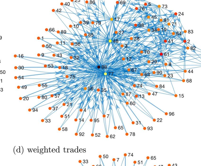
Figure 8. Networks of impacts with the entropy 0.6hIij i < Iij ≤ 0.75hIij i in (a)
case of all trades, (b) case of single trades, (c) case of multiple trades and (d) case of
weighted trades. The start of an arrow j → i represents the impacting stock j with
trading information and the end of the arrow represents the impacted stock i with price
changes. The colour of nodes indicates the connectivity of nodes. A positive value of
the connectivity is equal to the ingoing connectivity when it is larger than the outgoing
connectivity, while a negative value of the connectivity is equal to −1 multiplied by
the outgoing connectivity when it is larger than the ingoing connectivity.
100 60 14000
12000
40 10000
50 8000
20 6000
4000
0 0 2000
0 0
20 40 20 40
40 30 40 30
60 20 60 20
80 10 80 10
0 0
Figure 9. (a) Ingoing connectivity and (b) outgoing connectivity of each stock
depending on the group q. With the increase of q, the entropy of impacts increases and
the randomness increases. The colour indicates the average daily number of trades of
each stock.Grasping asymmetric information in market impacts 20
the network random with little structure. This demonstrates that the impact with small
entropy indeed reveals useful information. On the other hand, the stocks with a higher
ingoing connectivity have a smaller average daily number of trades, but the stocks with
a higher outgoing connectivity do not feature small number of trades. In particular,
the stocks with a large daily number of trades, e.g., AAPL indexed by 2, FB indexed
by 38, GILD indexed by 41, and MSFT indexed by 61, are more likely to impact other
stocks. The result that impacts are related to the number of trades is consistent with
the findings in Ref. [8], where another method of analysis was used.
6. Conclusions
By reconstructing the order book, we worked out the price cross-response, i.e., the price
change of one stock due to single trades or multiple trades of another stock. As we
focused on the immediate response, we used an event time scale. The cross-responses
are averaged over all trades, as well as over single trades, multiple trades and trades
weighted by the percentages of single trades and multiple trades. Distinguishing these
four types of cross-responses yields a detailed picture of the price impacts.
The distributions of cross-responses for the whole market show right skewness,
revealing the imbalance of positive and negative cross-responses. This implies that a
buy (or a sell) of one stock is very likely to move up (or down) the price of another stock.
The distributions are fitted well by stable distributions. The fit parameters reflect the
asymmetry and may be interpreted as measuring the degree of non-randomness of the
events. By quantifying the asymmetry for the cross-responses, we found that the impact
from stock j to i is not equal to the one from stock i to j. This corroborates the findings
in Ref. [15] and hints at a possibility for arbitrage when ignoring the bid-ask spread.
We also evaluated eigenvalue spectra of asymmetric impact structures. The results
demonstrate that the information encoded in the asymmetric impact structures is not
fully random. The Shannon entropy [25] reveals that the cases of single trades and
of weighted trades contain more non-random information than others. We further
estimated the entropy of impacts, which is composed of the entropy of trading
information and of price changes. For a given entropy of impacts, we constructed
a directional network to visualize the impacts among stocks. The evolution of this
network discloses that impacts with small entropy are more informative. Furthermore,
the stocks with large daily numbers of trades are more likely to impact others while the
less frequently traded stocks tend to be impacted by others.
We identified, quantified and visualized the asymmetric information in price impacts
and found that (1) the impacts in the whole market are asymmetric and non-random;
(2) the randomness of impacts across stocks can be quantified by the entropy of impacts;
(3) informative impacts are present at small entropy; (4) the stocks with large (small)
number of trades are likely to affect (be affected by) others.Grasping asymmetric information in market impacts 21
Acknowledgments
We thank A. Becker, S. Krause, Y. Stepanov and D. Waltner for fruitful discussions.
References
[1] B. Mandelbrot, J. Bus. 36(4), 394 (1963)
[2] R. Cont, Quant. Finance 1(2), 223 (2001)
[3] T.A. Schmitt, R. Schäfer, M.C. Münnix, T. Guhr, Europhys. Lett. 100(3), 38005 (2012)
[4] X. Gabaix, P. Gopikrishnan, V. Plerou, H.E. Stanley, Nature 423(6937), 267 (2003)
[5] J.P. Bouchaud, Y. Gefen, M. Potters, M. Wyart, Quant. Finance 4(2), 176 (2004)
[6] F. Lillo, J.D. Farmer, R.N. Mantegna, Nature 421(6919), 129 (2003)
[7] S. Wang, R. Schäfer, T. Guhr, Eur. Phys. J. B 89, 105 (2016)
[8] S. Wang, R. Schäfer, T. Guhr, Eur. Phys. J. B 89, 207 (2016)
[9] J.P. Bouchaud, Price impact, in Encyclopedia of Quantitative Finance (John Wiley & Sons,
Hoboken, NJ, 2010)
[10] H. Demsetz, Q. J. Econ. 82(1), 33 (1968)
[11] F. Lillo, S. Mike, J.D. Farmer, Phys. Rev. E 71(6), 066122 (2005)
[12] R. Almgren, C. Thum, E. Hauptmann, H. Li, Risk 18(7), 58 (2005)
[13] N. Torre, BARRA Inc., Berkeley (1997)
[14] M. Benzaquen, I. Mastromatteo, Z. Eisler, J.P. Bouchaud, J. Stat. Mech. Theor. Exp. 2017(2),
023406 (2017)
[15] M. Schneider, F. Lillo, Quantitative Finance (2018)
[16] S. Wang, arXiv:1701.03098 (2017)
[17] I. Mastromatteo, M. Benzaquen, Z. Eisler, J.P. Bouchaud, Risk July 2017 (2017)
[18] J. Gatheral, Quant. Finance 10(7), 749 (2010)
[19] J. Gatheral, A. Schied, A. Slynko, Math. Finance 22(3), 445 (2012)
[20] J. Gatheral, A. Schied, Dynamical models of market impact and algorithms for order execution,
in HANDBOOK ON SYSTEMIC RISK, edited by J.P. Fouque, J. A. Langsam (Cambridge
University Press, Cambridge, 2013), pp. 579–599
[21] A.A. Obizhaeva, J. Wang, J. Financ. Mark. 16(1), 1 (2013)
[22] A. Alfonsi, J.I. Acevedo, Appl. Math. Finance 21(3), 201 (2014)
[23] A. Alfonsi, P. Blanc, Finance Stochastics 20(1), 183 (2016)
[24] S. Wang, T. Guhr, arXiv:1609.04890 (2016)
[25] C.E. Shannon, Bell Syst. Tech. J. 27, 623 (1948)
[26] TAQ 3 User’s Guide, New York Stock Exchange, Inc., 1. 1. 9 edn. (2008)
[27] http://www.tradingphysics.com
[28] J. Nolan, Stable distributions: models for heavy-tailed data (Birkhauser, New York, 2003)
[29] L. Laloux, P. Cizeau, J.P. Bouchaud, M. Potters, Phys. Rev. Lett. 83(7), 1467 (1999)
[30] L. Laloux, P. Cizeau, M. Potters, J.P. Bouchaud, Int. J. Theoretical Appl. Finance 3(03), 391
(2000)
[31] V. Plerou, P. Gopikrishnan, B. Rosenow, L.N. Amaral, H.E. Stanley, Physica A 287(3), 374 (2000)
[32] V. Plerou, P. Gopikrishnan, B. Rosenow, L.A.N. Amaral, T. Guhr, H.E. Stanley, Phys. Rev. E
65(6), 066126 (2002)
[33] M. Potters, J.P. Bouchaud, L. Laloux, Acta Physica Polonica B 36(9), 2767 (2005)
[34] J.P. Bouchaud, M. Potters, arXiv:0910.1205 (2009)
[35] V.A. Marčenko, L.A. Pastur, Math. USSR-Sb. 1(4), 457 (1967)
[36] J.W. Silverstein, Z. Bai, J. Multivariate Anal. 54(2), 175 (1995)
[37] A.M. Sengupta, P.P. Mitra, Phys. Rev. E 60(3), 3389 (1999)
[38] H. Sommers, A. Crisanti, H. Sompolinsky, Y. Stein, Phys. Rev. Lett. 60(19), 1895 (1988)22
[39] E.N. Suparno, S.K. Jo, K. Lim, A. Purqon, S.Y. Kim, Group identification in Indonesian stock
market, in Journal of Physics: Conference Series (IOP Publishing, 2016), Vol. 739, p. 012037
[40] E.F. Fama, J. Financ. 25(2), 383 (1970)
[41] S.J. Grossman, J.E. Stiglitz, Am. Econ. Rev. 70(3), 393 (1980)
[42] A.W. Lo, J. Portfolio Manage. 30(5), 15 (2004)
Appendices
A. Trading data
By order reconstruction, we filter the trade and quote data to a resolution of one
millisecond. Table A.1 lists the daily numbers of trades and quotes and the spread
between the best ask and bid for 96 stocks in NASDAQ 100 index. The data is measured
during intraday trading time from 9:40 to 15:50 EST and averaged over five trading days
from March 7th to March 11th in 2016.23
Table A.1. Daily trade and quote information averaged over five trading days
Stock Number Number Spread Stock Number Number Spread
No. No.
symbol of trades of quotes (dollars) symbol of trades of quotes (dollars)
1 AAL 4,563 86,481 0.013 49 JD 3,596 64,622 0.012
2 AAPL 13,598 312,068 0.012 50 KHC 3,140 45,201 0.027
3 ADBE 4,553 41,067 0.034 51 KLAC 1,803 53,830 0.014
4 ADI 2,931 30,598 0.023 52 LBTYA 2,759 60,328 0.013
5 ADP 2,954 59,388 0.023 53 LLTC 2,300 59,533 0.014
6 ADSK 3,389 33,981 0.032 54 LMCA 1,585 30,686 0.016
7 AKAM 2,439 37,125 0.024 55 LRCX 3,826 40,132 0.038
8 ALXN 2,466 25,072 0.212 56 LVNTA 1,063 10,127 0.046
9 AMAT 2,066 61,402 0.010 57 MAR 3,495 54,363 0.024
10 AMGN 5,132 31,036 0.083 58 MAT 2,918 50,904 0.012
11 AMZN 5,376 54,185 0.428 59 MDLZ 3,666 74,011 0.011
12 ATVI 3,882 110,135 0.011 60 MNST 1,591 12,606 0.123
13 AVGO 5,518 39,476 0.095 61 MSFT 9,245 164,847 0.011
14 BBBY 2,590 29,066 0.026 62 MU 2,351 62,667 0.010
15 BIDU 2,729 18,414 0.191 63 MYL 5,969 56,840 0.017
16 BIIB 2,818 21,057 0.273 64 NFLX 9,164 73,919 0.049
17 BMRN 2,135 17,778 0.180 65 NTAP 2,210 54,022 0.012
18 CA 1,531 37,172 0.011 66 NVDA 2,935 78,995 0.011
19 CELG 6,742 45,181 0.056 67 NXPI 3,824 34,424 0.056
20 CERN 3,440 34,198 0.022 68 ORLY 1,837 21,748 0.349
21 CHKP 2,030 15,733 0.048 69 PAYX 1,838 41,534 0.013
22 CHRW 2,021 19,541 0.032 70 PCAR 3,315 38,421 0.019
23 CHTR 2,650 20,287 0.189 71 PCLN 1,029 17,369 2.525
24 CMCSA 5,984 179,820 0.011 72 QCOM 7,030 117,669 0.011
25 COST 3,487 21,260 0.059 73 REGN 1,300 13,691 0.883
26 CSCO 3,273 106,513 0.011 74 ROST 3,868 61,006 0.016
27 CTSH 4,823 54,413 0.016 75 SBAC 1,935 19,128 0.084
28 CTXS 2,477 22,161 0.053 76 SBUX 5,719 111,888 0.012
29 DISCA 3,152 72,949 0.012 77 SIRI 514 310,522 0.010
30 DISH 2,261 27,956 0.026 78 SNDK 3,687 43,642 0.021
31 DLTR 4,021 26,372 0.037 79 SPLS 1,108 37,419 0.010
32 EA 4,708 53,137 0.021 80 SRCL 1,588 11,546 0.094
33 EBAY 2,850 69,949 0.011 81 STX 4,056 39,986 0.017
34 EQIX 1,615 32,672 0.408 82 SYMC 1,784 41,076 0.010
35 ESRX 6,144 64,200 0.020 83 TRIP 3,473 23,576 0.050
36 EXPD 2,310 32,064 0.015 84 TSCO 1,535 15,998 0.073
37 FAST 2,816 32,818 0.018 85 TSLA 3,367 19,876 0.277
38 FB 14,921 213,281 0.016 86 TXN 3,479 81,678 0.012
39 FISV 1,856 22,382 0.043 87 VIAB 3,769 35,708 0.023
40 FOXA 2,388 66,595 0.010 88 VIP 217 6,494 0.010
41 GILD 11,681 95,291 0.016 89 VOD 926 62,212 0.011
42 GOOG 4,426 40,123 0.515 90 VRSK 1,264 11,367 0.044
43 GRMN 1,909 30,404 0.017 91 VRTX 3,037 19,411 0.129
44 HSIC 674 13,076 0.226 92 WDC 6,662 61,126 0.026
45 ILMN 1,860 16,979 0.266 93 WFM 3,775 63,946 0.012
46 INTC 3,933 115,962 0.011 94 WYNN 4,046 26,083 0.081
47 INTU 2,299 23,210 0.053 95 XLNX 2,450 33,769 0.016
48 ISRG 616 13,015 1.269 96 YHOO 6,258 134,390 0.011You can also read