University of Otago Economics Discussion Papers No. 1503
←
→
Page content transcription
If your browser does not render page correctly, please read the page content below
ISSN 1178-2293 (Online)

                                                 University of Otago
                                         Economics Discussion Papers
                                                            No. 1503
                                                          APRIL 2015

 Is New Zealand’s economy vulnerable to world oil market shocks?

                   Mohammad Jaforullah and Alan King

Address for correspondence:
Mohammad Jaforullah
Department of Economics
University of Otago
PO Box 56
Dunedin
NEW ZEALAND
Email: mohammad.jaforullah@otago.ac.nz
Telephone: 64 3 479 8731
Is New Zealand’s economy vulnerable to world oil market shocks?
a b
Mohammad Jaforullah and Alan King
a
Department of Economics, University of Otago, PO Box 56, Dunedin 9054, New Zealand.
Phone: +64-3-4798731. Email: mohammad.jaforullah@otago.ac.nz (Corresponding author)
b
Department of Economics, University of Otago, PO Box 56, Dunedin 9054, New Zealand.
Email: alan.king@otago.ac.nz
Abstract
We assess New Zealand’s vulnerability to oil shocks by estimating its price and income
elasticities of demand for imported oil and by testing for Granger causality between oil
imports, their price and GDP. Based on data for the period 1987Q2–2012Q4, we find the
short-run price and income elasticities to be statistically insignificant. However, the long-run
price and income elasticity estimates are significant and equal to −0.34 and 1.61,
respectively. We also find that oil imports, and to some extent oil prices, Granger-cause real
GDP, indicating that the New Zealand economy is vulnerable to shocks in the world oil
market.
Keywords: Oil imports; Price elasticity; Income elasticity; Granger causality; Cointegration;
Vector error correction model.
JEL classifications: C32, Q41, Q43
Acknowledgements
The authors would like to thank Alfred Haug and Dorian Owen for their helpful comments on
an earlier version of this paper. They also wish to thank Byeongseon Seo for providing the
GAUSS programmes for his tests. However, the authors are solely responsible for any
remaining errors.
11. Introduction
Oil is the single largest source of energy consumed within the New Zealand (NZ) economy,
accounting for 34% of its total primary energy supply in 2011. NZ produces some oil, but
most of this is exported, as it is lighter and sweeter than is suitable for its only oil refinery at
Marsden Point. In any case, indigenous crude oil production normally represents a relatively
small fraction of domestic oil consumption. For example, NZ’s net oil dependency, defined
as one minus the ratio of indigenous crude oil production to total domestic oil consumption,
was 62% in 2011 (Ministry of Economic Development, 2013a). Consequently, NZ largely
depends on imported oil to satisfy domestic demand. These imports are processed at the
Marsden Point refinery before being distributed to consumers as petrol, diesel, aviation fuel,
fuel oil, bitumen and other petroleum products. The refinery supplies around 70% of New
Zealand’s petrol and diesel demand, which is supplemented by imports of refined petroleum
products.
The oil shocks of 1973 and 1979 clearly highlight the danger of being dependent on foreign
oil supplies and the possibility of future supply-side shocks cannot be ruled out. NZ
consumers of petroleum products would clearly be adversely affected by such an event, but it
is less clear whether the economy as a whole would be noticeably affected. It is possible that
the high oil prices experienced in the 1970s encouraged structural change within the economy
that has enhanced its ability to cope with such events. So, it is an open question whether
economic activity in NZ is currently vulnerable to shocks originating in the world oil market.
The extent to which an economy is sensitive to such shocks depends, in part at least, on its
price elasticity of demand for oil. A low elasticity indicates that consumers have little ability
to reduce their dependence on oil when its price rises – by either improving efficiency or
switching to alternative energy sources – and this increases the risk to economic activity. An
economy’s vulnerability to oil shocks can also be assessed by testing for a Granger-causal
relationship between the level of oil imports and the level of economic activity, i.e., real gross
domestic product (GDP). If oil imports Granger-cause GDP, then this indicates that supply-
side disruptions to the global oil market have the potential to harm domestic economic
activity.
Therefore, this paper estimates the short- and long-run price (and income) elasticities of
demand for oil imported into NZ and also examines the nature of Granger causality, if it
2exists, between oil imports and NZ’s GDP. The issue of the NZ economy’s vulnerability to
disruptions in oil imports has not been previously investigated to our knowledge, although
Granger causality between oil consumption (rather than imports) and GDP, and the price
elasticity of oil imports have been examined separately (Cooper, 2003; Fatai et al., 2004).
Both of these earlier studies, however, have some limitations that have the potential to affect
their conclusions and our study seeks to address these limitations.
The remainder of the paper is organised as follows. Section 2 reviews the empirical literature
that models the demand for oil imports and considers the Granger-causal relationship
between oil imports and GDP, with particular emphasis on the studies that consider the NZ
case. In Section 3, the data and methodology we employ are discussed, and the elasticity
estimates and the Granger-causality test results they produce are presented in Section 4.
Section 5 concludes the paper by highlighting the main empirical findings and outlining their
policy implications.
2. Literature review
There are numerous studies of the causal relationship between energy consumption and
economic growth. Some specifically focus on the causal relationship between the
consumption of oil and economic growth, and a subset of these also estimate short- and long-
run price and income elasticities of demand for oil imports. The studies within this last
group, however, do differ in terms of the specific variables included in their model and/or the
econometric methodology they employ to analyse it.
For example, Ghosh (2009) and Royfaizal (2009) both estimate an Autoregressive
Distributed Lag (ARDL) model of the demand for imported oil in India and Japan,
respectively, and use the Bounds test (Pesaran and Shin, 1999; Pesaran et al., 2001) to
determine whether the variables within their model have a long-run equilibrium (or
cointegrating) relationship. Their choice of the Bounds test is based on the fact that it can be
applied regardless of whether the individual variables are all stationary, all integrated of order
one, or some combination of the two (Pesaran et al., 2001). In addition, the Bounds test is
expected to generate robust results for relatively small samples (Pesaran and Shin, 1999).
If a cointegrating relationship is found then, aside from providing estimates of the long-run
price and income elasticities of demand for imported oil, it can also be used to construct the
3error- (or equilibrium-) correction term within a Vector Error Correction model (VECM).
Both studies are able to do this and use their VECM to examine the direction of Granger
causality between oil imports and real GDP, and to generate estimates of the short-run price
and income elasticities of demand for oil imports.
However, these two studies differ in that Ghosh (2009) models the relationship between the
volume of oil imports, the real price of oil and real GDP, whereas Royfaizal (2009) models
the volume of oil imports, the nominal price of oil and real GDP. When modelling import
demand it is standard practice to control for the effects on the demand for one good of
changes in the prices of other goods (Goldstein and Khan, 1985; Sawyer and Sprinkle, 1999).
This is often done – as Ghosh (2009) does – by deflating the imported good’s own price by a
broadly-defined price index (e.g., a GDP deflator or a consumers price index). Hence,
Royfaizal’s (2009) results need to be interpreted in the light of his nonstandard approach.
Ghosh’s (2009) estimate of the long-run income elasticity of India’s oil imports demand is
1.97. His estimates of both the short- and long-run price elasticities, and the short-run
income elasticity are all statistically insignificant. Royfaizal’s (2009) estimates of the long-
run price and income elasticities of Japanese demand for oil imports are −0.08 and 1.35,
respectively. However, his estimate of the short-run income elasticity is noticeably larger at
1.78, which is contrary to theoretical expectations and may be a reflection of his model’s
omission of a broadly-defined price variable. With respect to the pattern of Granger causality
between oil imports and real GDP, the findings of the two studies are the same: real GDP is
found to Granger-cause oil imports without feedback in both India and Japan.
Other studies to use the ARDL modelling approach and the Bounds test for cointegration to
obtain estimates of the price and income elasticities of demand for imported oil, but which do
not explore the issue of Granger causality, include Altinay (2007), Asali (2011) and Moore
(2011). Altinay’s (2007) study considers the case of Turkey and uses annual data (for the
period 1980–2005). Two alternative price variables are considered for use (alongside real
GDP) in Turkey’s import demand equation: the real price of oil and the nominal oil price
expressed in US dollar terms. Only the model containing the latter measure is found to
generate significant evidence of cointegration and, on this basis, Altinay (2007) estimates
Turkey’s short-run (long-run) price elasticity of demand for oil to be −0.10 (−0.18) and its
income elasticity to be 0.64 (0.61).
4Asali (2011) estimates the price and income elasticities of the G7 nations along with those of
Brazil, Russia, India and China. The model employed in this study differs slightly from those
mentioned above in that all variables, except the real price of oil, are defined in per capita
terms. The price elasticity estimates found are relatively consistent across the countries in the
sample, ranging from −0.02 to −0.10 in the short run and from −0.05 to −0.18 in the long run.
Considerably greater variation, however, is found among the income elasticity estimates,
which range from 0.11 to 0.89 in the short run and from 0.35 to 1.35 in the long run.
Moore’s (2011) study of oil import demand in Barbados differs from the others in that it is
based on a relatively short span (1998–2009) of monthly data. He reports a long-run price
elasticity of demand for oil of −0.55, whereas the long-run effect of income on import
demand is not found to be statistically significant. However, the latter finding is likely to be
a reflection of the inclusion of electricity consumption as an explanatory variable in Moore’s
(2011) import demand model, given that almost half of all oil imported by Barbados is used
for electricity generation
Not all researchers in this area have used the ARDL model-based Bounds test approach.
Ziramba (2010), for example, uses Johansen’s (1988, 1991, 1995) maximum likelihood
method to estimate the long-run relationship between South Africa’s volume of oil imports
and its determinants, namely real GDP and the real oil price. Based on annual data for the
period 1980–2006, his estimates of the long-run price and income elasticities for South Africa
are −0.15 and 0.43, respectively. (The short-run elasticity estimates are not reported.) To test
the direction of Granger causality between the variables, Ziramba (2010) estimates a VECM
containing an error-correction term based on the single long-run cointegrating vector
identified by his Johansen test results. In common with Ghosh (2009) and Royfaizal (2009),
Ziramba (2010) also finds a unidirectional causal relationship running from real GDP to oil
imports.
Very little work appears to have been done on the determinants of NZ’s demand for imported
oil or on the relationship between its oil imports and economic activity. Only two studies, to
our knowledge, attempt to tackle either issue. As part of a multi-country study, Cooper
(2003) estimates a simple partial-adjustment model of per capita oil import demand for NZ
(over the period 1971–2000) and obtains short- and long-run price elasticities of −0.054 and
−0.326, respectively. (Per capita real GDP is included in the model but the income elasticity
5estimates are not reported.) However, the time-series properties of the data set are not tested
and no test for cointegration is undertaken. Therefore, as at least some of the model’s
variables are likely to be non-stationary, Cooper’s (2003) results may be subject to the
spurious regression problem (Granger and Newbold, 1974).
Fatai et al. (2004) test for Granger causality between NZ’s real GDP and its level of oil
consumption using data for the period 1960–1999. Based on the results of the Johansen
testing approach, they are unable to find evidence of cointegration between the two series and
so test for Granger causality using first-differenced data only. On this basis they find no
evidence of causality in either direction. However, their cointegration test results – and hence
their Granger-causality test results – may have been affected by the exclusion of an oil price
variable from the proposed cointegrating vector.
A further point to consider is that both Cooper (2003) and Fatai et al. (2004) make use of data
that straddles the period of the original oil shocks. Hence, it is possible that their results may
be distorted by any structural changes to the NZ economy that occurred in response to those
shocks. One indicator of a possible structural change is the share of oil in NZ’s total primary
energy supply, which fell from 49% in 1974 to 31% by 1985. Over the same period, NZ’s
net oil dependency also fell, from 95% to 63%. Both measures subsequently fluctuate in
value, but they have nonetheless remained close to their 1985 levels over the last quarter-
century. Specifically, the average values of oil’s share in the primary energy supply and net
oil dependency over the period 1985–2011 are 33% and 62%, respectively (Ministry of
Economic Development, 2013a). Given the change in the NZ economy’s reliance on oil in
general, and imported oil in particular, over the decade following the first oil shock, the aim
of the present study is to assess NZ’s current vulnerability to oil shocks through the use of
data and methods that address our concerns with the existing studies.
3. Methodology and data
3.1 Methodology
Crude oil is not directly consumed within an economy, except by industries producing oil-
based products such as plastic. Most oil is refined into other products, such as petrol, diesel,
fuel oil, bitumen, etc., and these are then consumed by all sectors of the economy. Standard
theories of production and consumption suggest that the total amount of crude oil demanded
6should therefore depend on the level of economic activity, the conventional measure of which
is real GDP, the price of oil itself and the prices of substitute products.
Outside of, arguably, electricity generation (which in NZ is dominated by hydroelectric
generation in any case) and central heating systems (which are not a common feature of NZ’s
housing stock), fossil fuels such as coal and natural gas are typically not good substitutes for
oil and its refined products given the current state of technology and the existing stock of
capital. Therefore, and in common with most previous studies in this area, substitute prices
are represented by a general price index (which we use to deflate the nominal oil price),
rather than one defined over non-oil energy sources alone.
Assuming a log-linear relationship among the variables, our model of demand for imported
oil is as follows:
LOIMPt = θ0 + θ1LRGDPt + θ2LRPOILt + ut (1)
where LOIMP is the logarithm of the volume of oil imports, LRGDP is the logarithm of real
GDP, LRPOIL is the logarithm of the real price of oil and u is a random error. Equation (1)
represents the long-run relationship among the variables and so θ1 is interpreted as the long-
run income elasticity and θ2 as the long-run price elasticity of demand for oil imports. The
value of θ1 is expected to be positive and that of θ2 negative.
Even though equation (1) looks simple and straightforward, econometric problems may be
encountered when estimating it. One potential problem is that, although the nominal (i.e., US
dollar) price of oil is set on the world market and so can be considered exogenously
determined from NZ’s perspective, the real price of oil faced by NZ consumers also depends
on the NZ dollar’s exchange rate against the US dollar and on domestic inflation, both of
which could be influenced by the state of the NZ economy (i.e., LRGDP). In which case,
LRPOIL may not be entirely exogenously determined. Moreover, the theory of production
suggests that LRGDP itself may also be an endogenous variable, as oil is an input into
production and so shocks to LOIMP may be reflected in LRGDP. Therefore, there is some
risk of simultaneity bias if equation (1) is estimated using ordinary least squares. This can be
avoided if a vector autoregressive (VAR) modelling approach is employed instead.
When equation (1) is transformed into a VAR model format it takes the following form:
7p p p
a10 + ∑ a1i LOIMPt −i + ∑ b1i LRGDPt −i + ∑ c1i LRPOILt −i + u1t
LOIMPt =
=i 1 =i 1 =i 1
p p p
a20 + ∑ a2i LOIMPt −i + ∑ b2i LRGDPt −i + ∑ c2i LRPOILt −i + u2t
LRGDPt = (2)
=i 1 =i 1 =i 1
p p p
a30 + ∑ a3i LOIMPt −i + ∑ b3i LRGDPt −i + ∑ c3i LRPOILt −i + u3t
LRPOILt =
=i 1 =i 1 =i 1
where LOIMP, LRGDP and LRPOIL are as defined above, uit is the random error term for the
i-th equation and time period t, and p is the lag length of the VAR. This format of the model,
however, is only valid if LOIMP, LRGDP and LRPOIL are all individually integrated of order
zero, i.e., I(0). If this is not the case – specifically, if they are integrated of order d, I(d), and
are not cointegrated – then all terms in equation (2) must be differenced d times prior to
estimation. On the other hand, if the variables are I(d) but are cointegrated, then an error-
correction term derived from the cointegrating relationship must be included in the model in
addition to dth-differenced variables. For example, in the case where all variables are I(1)
and have only one valid cointegrating relationship, the appropriate model is a VECM of the
following form:
p −1 p −1 p −1
DLOIMPt =a10 + ∂1ECTt −1 + ∑ a1i DLOIMPt −i + ∑ b1i DLRGDPt −i + ∑ c1i DLRPOILt −i + u1t
=i 1 =i 1 =i 1
p −1 p −1 p −1
DLRGDPt =a20 + ∂ 2 ECTt −1 + ∑ a2i DLOIMPt −i + ∑ b2i DLRGDPt −i + ∑ c2i DLRPOILt −i + u2t (3)
=i 1 =i 1 =i 1
p −1 p −1 p −1
DLRPOIL=
t a30 + ∂ 3 ECTt −1 + ∑ a3i DLOIMPt −i + ∑ b3i DLRGDPt −i + ∑ c3i DLRPOILt −i + u3t
=i 1 =i 1 =i 1
where ∆ is the first-difference operator and ECT is the error-correction term. ECT represents
the deviation from the long-run, or cointegrating, relationship among the variables – i.e.,
ECTt = LOIMPt − θ0 − θ1LRGDPt − θ2LRPOILt, where the cointegrating vector is normalised
on LOIMP. If the lagged error-correction term is not included in the model, it will suffer
from specification error (Engle and Granger, 1987).
If, for example, the null hypothesis that ∂1 = 0 can be rejected, this implies that LOIMP
changes in response to shocks that cause a deviation from the long-run equilibrium
relationship (i.e., ECT ≠ 0). As this relationship is normalized on LOIMP, ∂1 is expected to
take a value between 0 and −1, as it denotes the fraction of the deviation from the long-run
equilibrium observed in period t−1 that is expected to be ‘corrected’ in period t. If the other
adjustment parameters, ∂2 and ∂3, prove to be non-zero, this indicates that LRGDP and
8LRPOIL, respectively, are also sensitive to shocks that disturb the system’s long-run
equilibrium – i.e., they are endogenously determined. However, if the null hypothesis that ∂2
= 0 (∂3 = 0) cannot be rejected, it can be concluded that LRGDP (LRPOIL) is weakly
exogenous in the context of the model.
Therefore, to choose the correct model, one must first determine the order of integration of
each variable in equation (1) by means of a unit-root test. If some or all of these variables are
found to be individually non-stationary, it then becomes necessary to determine whether they
are cointegrated – i.e., there exists a linear combination of the variables that is stationary.
We use the Johansen (1988, 1991, 1995) approach to test for cointegration in preference to
the Bounds test for the following reasons. First, as it tests for cointegration within a VAR
framework, the Johansen method does not require the variables within the proposed
cointegrating vector (other than the selected dependent variable) to satisfy a weak-exogeneity
assumption (which, as mentioned above, may be problematic in the present context). Instead,
all are initially treated as if they are endogenously determined and their actual status is
evaluated subsequently. Second, because the Johansen test uses a systems estimation method
it has the advantage of allowing the number of cointegrating relationships to be determined
by the data, rather than assuming there is (at most) only one such relationship, as is done in
the Bounds test. Finally, our sample size is reasonably large (T = 103), which somewhat
lessens the advantage the Bounds test can have over the Johansen methodology in relation to
small samples.
Engle and Granger (1987) demonstrate that, if there is evidence of a cointegration among a
set of variables, it implies that there is Granger causality between those variables in at least
one direction. Granger causality implies that the past and present values of one variable can
help to improve the forecasts of another (Granger, 1969). The existence and direction of
causation between any pair of variables from within the cointegrating relationship can be
assessed by estimating a VECM that incorporates an error-correction term derived from that
relationship (Granger, 1986; 1988). Specifically, evidence of Granger causality running from
one variable, X, to another, Y, may be obtained by a joint test of the significance (in the
VECM’s regression equation with ΔY as the dependent variable) of the ECT and the lags of
ΔX (Enders, 2004, 334). For example, if after estimating equation (3) the null hypothesis that
∂1 = b11 = ... = b1,p−1 = 0 can be rejected, then LRGDP can be said to Granger-cause LOIMP.
9If it is also possible to reject the null that ∂2 = a21 = ... = a2,p−1 = 0, then LOIMP can be said to
Granger-cause LRGDP – i.e., there is bi-directional causality (or causality with feedback)
between these two variables. Each of these null hypotheses can also be tested as two separate
hypotheses – e.g., ∂1 = 0 and b11 = ... = b1,p−1 = 0. In this way it can be determined whether
the source of Granger causality is the process of adjustment back to the long-run equilibrium
relationship and/or the VECM’s short-run dynamics, respectively.
3.2. Data
Our data set contains quarterly observations of each variable for the period 1987Q2–2012Q4.
The choice of the sample period is dictated by the availability of some key data series but, as
it falls some time after the two major oil shocks of the 1970s, it has the advantage of reducing
the risk of structural changes in the relationships between the variables distorting our
econometric results.
Data on the volume of NZ’s oil imports are obtained from the Ministry of Business,
Innovation and Employment (2013). The quarterly oil imports are in gross petajoules (PJ),
which are converted into barrels of oil equivalent at the rate of 1.634×10⁵ barrels per PJ. The
price of West Texas Intermediate (WTI) 40 API, Midland Texas, is used as a proxy for the
world price of oil. The WTI price series is highly correlated with other oil price series and, as
Asali (2011, p. 192) notes, “... one can assume the existence of one global price for crude oil,
such that using WTI in demand for oil equations of sample countries as a proxy for their
domestic crude oil price would not cause any significant problem from a statistical point of
view.” Data on the WTI price in US dollars per barrel are obtained from the International
Monetary Fund’s International Financial Statistics database (http://www.imf.org/external/
data.htm), as is the US$/NZ$ exchange rate used to convert the WTI series into NZ dollar
terms. The real oil price series is then obtained by deflating the nominal series with the
Consumer Price Index taken from Statistics New Zealand’s Infoshare database
(www.stats.govt.nz/infoshare/), which is also the source of the real (seasonally adjusted)
GDP series. Summary statistics of the three variables are presented in Table 1. Note that the
real GDP and the real price of oil series have different base years, but this should not create
any difficulties as all series are converted in logarithmic terms prior to econometric testing.
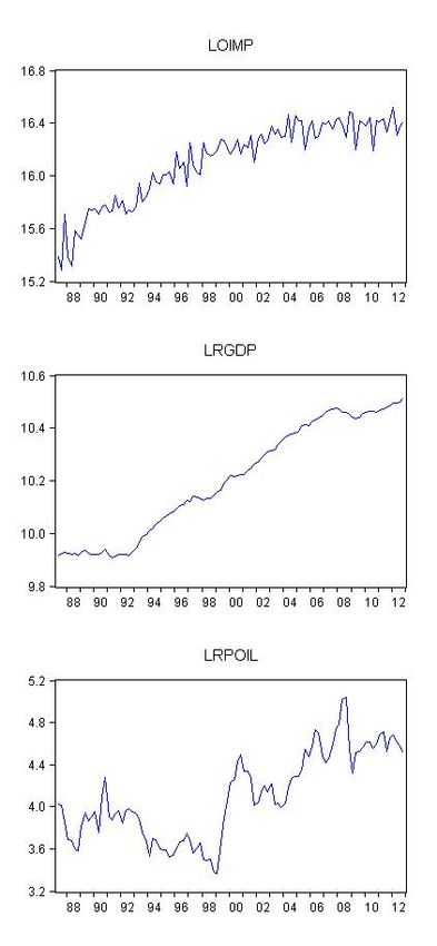
Plots of LOIMP, LRGDP and LRPOIL are shown in Figure 1
10Figure 1
Plots of LOIMP, LRGDP and LRPOIL
11Table 1
Descriptive statistics for all variables
Oil imports Real oil price Real GDP
(000s of barrels (2006 NZ$) (1995/96 NZ$m)
equivalent)
Mean 10,321.4 65.72 27,653
Median 10,846.9 56.26 27,363
Maximum 14,997.2 153.56 36,806
Minimum 4,343.0 28.84 20,113
Std. Dev. 2,778.1 27.70 5,788
Observations 103 103 103
4. Econometric results
4.1 Unit-root test results
To determine whether the variables have non-stationary data-generating processes, three unit-
root tests are employed: the Augmented Dickey-Fuller (ADF) test (Dickey and Fuller, 1981),
the Phillips-Perron (PP) test (Phillips and Perron, 1988) and the KPSS test (Kwiatkowski et
al., 1992). Under the ADF and PP tests, the null hypothesis is that the series in question has a
unit-root process, whereas the null hypothesis under the KPSS test is that it does not. In all
cases a linear time trend and a constant term have been included in the test equation. The
selection of the optimal lag length for each test equation is based on either the Schwarz
criterion (for the ADF test) or the Bartlett Kernel with a Newey-West bandwidth (for the PP
and the KPSS tests). The results obtained for each test are presented in Table 2.
All three unit-root tests agree on the time-series properties of LRGDP and LRPOIL, in that
their first-differences are stationary, but when expressed in levels terms they exhibit a unit
root. Therefore, we conclude that both series are I(1). The PP test results for LOIMP,
however, contradict those for the ADF and KPSS tests. The PP test finds evidence that this
series is stationary in levels, whereas the other two tests indicate that only its first-difference
is stationary. As there is some evidence that LOIMP has a unit root, we err on the side of
caution and decide to treat it as an I(1) series. Hence, with all three variables considered to
be I(1), it is necessary to establish whether they are cointegrated, i.e., whether there is at least
one linear combination of these variables that is stationary.
12Table 2
Unit-root test results
Variable ADF test PP test KPSS test
LRGDP –2.0018 (1) –1.9737 (6) 0.1310* (8)
ΔLRGDP –6.7987*** (0) –6.8813*** (3) 0.1615 (6)
LOIMP –1.5903 (3) –6.7544*** (8) 0.3012*** (8)
ΔLOIMP –13.3166*** (2) –31.8379*** (8) 0.0441 (7)
LRPOIL –2.8461 (0) –2.9488 (2) 0.1821** (8)
ΔLRPOIL –8.5655*** (1) –8.5743*** (4) 0.0511 (4)
Notes: *** (**) [*] indicates rejection of the null hypothesis at the 1% (5%) [10%] level. Numbers in
parentheses are the lag length for the ADF test and bandwidth for the PP and KPSS tests. Δ denotes the first-
difference operator.
4.2 Johansen cointegration test results
The first step when applying the Johansen cointegration test is to determine the optimal lag
length of the underlying VAR model, i.e., the value of p in equation (2). We follow the
optimal lag selection procedure suggested by Enders (2004, pp. 358-359). Specifically, an
unrestricted VAR model with p = 5 (= T1/3) is initially estimated and then shorter lag lengths
are considered. Several lag selection criteria – including a sequential modified LR test
statistic, the Final Prediction Error, the Akaike Information Criterion and the Hannan-Quinn
Information Criterion – suggest that the optimal lag is p = 4.
The Johansen methodology generates two tests for cointegration: the trace and maximum-
eigenvalue cointegration rank (r) tests. The trace test statistic (λtrace) evaluates the null
hypothesis that there are, at most, r cointegrating vectors against the alternative that they
number more than r. The maximum-eigenvalue (λmax) test is more specific in that its null
hypothesis is that there are r cointegrating vectors and the alternative is that there are r + 1
cointegrating vectors. Both tests begin by setting r = 0 and then progressively increase its
value until the null hypothesis cannot be rejected. The results obtained are shown in Table 3.
Both the λtrace and λmax test statistics indicate that there is only one cointegrating vector among
the three variables under study and this equation is shown – normalised on LOIMP – in Table
3. As this equation can be considered to represent the long-run equilibrium relationship
13among the variables, the coefficients on LRPOIL and LRGDP are estimates of NZ’s long-run
price and income elasticities of demand for imported oil. Both estimates have their expected
sign and are significantly different from zero at the 1% level of significance. The value of the
long-run income elasticity is 1.61, which is comparable to the values found for India (1.97;
Ghosh, 2009), France, Italy (1.35 and 1.32, respectively; Asali, 2011) and Japan (1.35;
Royfaizal, 2009). The long-run price elasticity is inelastic as expected, and its value of −0.34
is also similar to the estimates found for most other countries.
Table 3
Johansen test for cointegration results
(a) Trace test:
H0 H1 λtrace p-value
r=0 r≥1 37.3690 0.0055
r≤1 r≥2 9.8099 0.2956
r≤2 r=3 1.5275 0.2165
(b) Maximum-eigenvalue test:
H0 H1 λmax p-value
r=0 r=1 27.5592 0.0054
r=1 r=2 8.2823 0.3507
r=2 r=3 1.5275 0.2165
(c) Cointegrating equation:
LOIMPt = −1.1333 − 0.3422 LRPOILt + 1.6056 LRGDPt
(−4.173)* (10.216)*
Notes: * indicates significance at the 1% level. Numbers in parentheses are t-values (underlying asymptotic
standard errors corrected for degrees of freedom are calculated using the formula in Boswijk, 1995).
4.3 Tests for structural change and nonlinearity
Our choice of sample period should reduce the risk of parameter instability in NZ’s oil import
demand relationship due to structural change, but it does not necessarily eliminate the risk.
Therefore, we apply Seo’s (1998) set of Lagrange Multiplier (LM) tests for structural change,
as they are specifically designed for models estimated by the maximum likelihood method
used in the Johansen approach. Specifically, Seo (1998) defines three LM statistics: the
average (Ave-LM), exponential average (Exp-LM) and the supremum (Sup-LM). All three
are based on the methods described by Andrews (1993) and Andrews and Ploberger (1994)
14and each can be used to test for structural change (at an unknown point) in either (a) the VAR
model’s adjustment vector (α, which defines its speed of adjustment to long-run equilibrium),
(b) the cointegrating vector (β, which defines the long-run equilibrium relationship between
the variables), or (c) both α and β jointly.
It is advisable to apply all three tests to evaluate each form of structural change as each has
different properties. In particular, the power of the Ave-LM test is concentrated on the
alternative that is near the null hypothesis, whereas that of the other two tests is concentrated
on more distant alternatives (Seo, 1998). Hence, rejection of the null hypothesis (of no
structural change) by any one of these tests would constitute evidence of structural change.
It should also be noted that the distribution of each test statistic is nonstandard due to the
presence of a nuisance parameter (i.e., the unknown point of structural change). Seo (1998)
provides suitable critical values for each test and these depend on the number of variables in
the cointegrating vector, its rank and the admissible range for the change point’s location
(i.e., the extent to which the endpoints of the sample period are excluded from the search for
the point of structural change).
The test results obtained are reported in Panel A of Table 4. All three test statistics fall well
short of their 5% critical value for each of all three forms of structural change considered.
Hence, we conclude there is no evidence of significant structural change in either NZ’s long-
run oil import demand relationship and/or its adjustment vector.
Another possible source of model misspecification worth considering is the assumption of
linearity in the adjustment process to the long-run equilibrium relationship that underlies the
Johansen test (in common with most other cointegration tests). It is possible that this
assumption is invalid and that the process actually takes a nonlinear form. For example,
adjustment may follow a smooth transition process (e.g., exponential, logistic, square-root,
quadratic, or logarithmic) or switch to a different regime when a particular threshold is
crossed. The appropriateness of the standard assumption of linearity in the cointegrating
β
vector’s error-correction process can be assessed by the specification error test (SETn)
proposed by Seo (2011).
15Table 4
Structural change and nonlinearity test results
(A) Structural change tests (Seo, 1998)
(a) Adjustment vector (α):
Test Test statistic 5% critical value
α
Ave-LMn 2.548 6.070
α
Exp-LMn 1.674 4.220
α
Sup-LMn 5.927 14.150
(b) Cointegrating vector (β):
Test Test statistic 5% critical value
β
Ave-LMn 0.920 4.320
β
Exp-LMn 0.498 3.240
β
Sup-LMn 2.313 12.550
(c) Joint tests (α and β):
Test Test statistic 5% critical value
βα
Ave-LMn 3.468 8.740
βα
Exp-LMn 2.254 6.130
βα
Sup-LMn 7.468 18.710
(B) Nonlinearity tests (Seo, 2011)
β
Polynomial order (k) SETn statistic p-value
2 2.4109 0.6607
3 2.4548 0.6527
4 2.4971 0.6452
5 2.5364 0.6381
Notes: The admissible range for all structural change tests is defined as [0.15T, 0.85T].
β
The SETn test evaluates the null hypothesis of the standard (i.e., linear) model of vector error
correction against an alternative model that allows for general nonlinear specifications of the
long-run relationship. In particular, the alternative model is constructed from the
polynomials (of order k) of the vector of nonstationary variables in the model and so does not
assume a specific nonlinear functional form. This implies that both smooth transition and
β
threshold cointegration models are contained within its specification (Seo, 2011). Our SETn
test statistics (for k = 2, 3, 4 and 5) are presented in Panel B of Table 4. They reveal no
significant evidence against the standard assumption of linear error correction.
164.4 VECM estimation results and tests for Granger causality
As the variables are integrated of the same order and are cointegrated, the appropriate basis
for testing Granger causality between oil imports and real GDP is the VECM described by
equation (3). This is estimated with p = 4 and its error correction term (ECT) defined by the
cointegrating relationship reported in Table 3. Following Altinay (2007), the model includes
a dummy variable (D) to control for the effects of the 1991 Gulf War. This dummy takes the
value of one in all quarters of 1991 and zero otherwise.
The estimated VECM is reported in Table 5. A range of standard diagnostic tests for
stability, heteroskedasticity, autocorrelation and error normality are applied to this model and
their results (which are not reported, but are available on request) reveal no significant
evidence of any undesirable statistical properties. It can be seen that the coefficient on
ECTt−1 is statistically significant in the oil imports equation alone, which implies that only the
quantity of oil imported adjusts in response to any deviation from the long-run equilibrium
relationship in order to re-establish the long-run relationship. This coefficient is negative, as
expected, and its magnitude implies that 34% of the deviation from the long-run equilibrium
relationship is eliminated in each quarter. The insignificance of the ECTt−1 terms in the other
two equations implies that both real GDP and real oil prices are weakly exogenously
determined in the context of this model.
The short-run price and income elasticities of NZ’s demand for imported oil are represented
by the coefficients on ΔLRPOIL(−1) and ΔLRGDP(−1), respectively, in the ΔLOIMP
equation. The value of the former is 0.09 and the latter is 0.78, but both estimates are
statistically insignificant. This implies that NZ’s demand for oil imports is slow to respond to
changes in both its level of economic activity and oil prices.
It is interesting to note that the estimated coefficient on the Gulf War dummy variable, D, is
negative and statistically significantly different from zero at the 5% level in the ΔLRGDP
equation in Table 5. This result suggests that the Gulf War in 1991 had adversely affected,
although to an economically small extent, the real GDP of NZ.
17Table 5
Vector error correction model estimates
Dependent variables
Independent variables ΔLOIMP ΔLRGDP ΔLRPOIL
ECT(−1) –0.3418** 0.0109 –0.2355
(–3.9328) (1.3521) (–1.7224)
ΔLOIMP(−1) –0.6970** 0.0148 0.2706
(–6.6761) (1.5191) (1.6472)
ΔLOIMP(−2) –0.6859** 0.0020 0.1981
(–6.6591) (0.2120) (1.2224)
ΔLOIMP(−3) –0.3844** 0.0161 –0.0215
(–4.3022) (1.9323) (–0.1531)
ΔLRGDP(−1) 0.7792 0.2910** –0.1444
(0.6967) (2.7976) (–0.0821)
ΔLRGDP(−2) –0.5152 0.1013 0.2952
(–0.4547) (0.9609) (0.1659)
ΔLRGDP(−3) –0.4239 0.0700 1.2371
(–0.3923) (0.6962) (0.7278)
ΔLRPOIL(−1) 0.0939 –0.0082 0.2620*
(1.3616) (–1.2819) (2.4156)
ΔLRPOIL(−2) 0.0409 –0.0126* –0.2544*
(0.6132) (–2.0269) (–2.4231)
ΔLRPOIL(−3) 0.0911 –0.0089 0.2195
(1.2992) (–1.3713) (1.9897)
CONSTANT 0.0253* 0.0035** –0.0035
(2.1571) (3.2031) (–0.1880)
D 0.0182 –0.0085* –0.0419
(0.4240) (–2.1351) (–0.6194)
Notes: Figures in parentheses are t statistics. ** (*) indicates statistical significance at the 1%
(5%) level in two-sided tests.
To determine the pattern of Granger causality within our VECM, Wald χ2 tests are conducted
and the results are reported in Table 6. These reveal evidence that oil imports are Granger-
caused by real GDP and the real price of oil through the error-correction process that re-
establishes the long-run equilibrium relationship, but not through the model’s short-run
dynamics. It can also be seen from Table 6 that oil imports Granger-cause real GDP through
the model’s short-run dynamics. The positive coefficient estimates for the lagged ∆LOIMP
terms within the ∆LRGDP equation in Table 5 indicate that this causal relationship is
18positive. Hence, disruptions to the supply of oil are expected to adversely affect real GDP in
the short run.
Table 6
Granger-causality test (Wald χ2) results
Sources of causation
Short-run Long-run Short-run plus long-run
Dependent ΔLOIMP ΔLRGDP ΔLRPOIL ECT ΔLOIMP ΔLRGDP ΔLRPOIL
variable + ECT + ECT + ECT
ΔLOIMP – 0.709 0.332 15.467** – 15.676** 15.658**
(0.871) (0.343) (0.000) (0.004) (0.004)
ΔLRGDP 8.855* – 7.562 1.828 15.248** – 7.568
(0.031) (0.056) (0.176) (0.004) (0.109)
ΔLRPOIL 4.340 0.726 – 2.967 5.252 4.081 –
(0.227) (0.867) (0.085) (0.262) (0.395)
Notes: ** indicates statistical significance of the test statistic at the 1% level. * indicates statistical significance at the
5% level. Figures in parentheses are p-values.
Table 6 also shows that the price of imported oil is not Granger-caused by either NZ’s real
GDP or its oil imports. This is as expected, as NZ is too small to have the economic or
political influence required to affect outcomes in the world oil market. However, the null
hypothesis that real GDP is Granger-caused by the real price of oil through the model’s short-
run dynamics can almost be rejected at the 5% level of significance. This result offers some
evidence that oil price shocks also have the ability to adversely affect economic activity in
the short run (as the coefficient estimates in Table 5 for the lagged ∆LRPOIL terms within the
∆LRGDP equation are negative).
5. Conclusions
This paper assesses the NZ economy’s vulnerability to shocks originating in the world market
for oil. These shocks can take the form of a sudden and dramatic rise in the price of oil or
disruptions to oil supplies caused by wars, natural calamities, or oil embargos by exporting
countries, etc. The oil price shocks of the 1970s highlighted the importance of this
commodity to the operation of most economies. Although efforts have been made to improve
energy efficiency and develop alternative energy sources since then, most economies are still
19very dependent on oil. NZ, in particular, has reduced its dependence on oil since 1973, but
nonetheless it still remains the single most important source of energy for the economy.
Through cointegration analysis and vector error correction modelling, we find the following
results. First, NZ’s demand for oil imports is price-inelastic in both the short and long run.
Specifically, in the short run there is no statistically discernible effect on demand in response
to a change in the world oil price. In the long run, the demand for imported oil will react, but
only by one-third of a percent for every one percent change in the price. Hence, in the event
of a dramatic rise in the oil price, NZ’s trade balance would be expected to fall sharply,
ceteris paribus. Second, there is evidence that oil imports, and possibly oil prices as well,
Granger-cause economic activity. Specifically, NZ’s real GDP is expected to be adversely
affected by disruptions to the availability of imported oil and increases in its price.
In summary, the NZ economy is still vulnerable to shocks originating in the world oil market.
Measures that can be taken to lessen the adverse effects of such shocks include the creation of
a strategic oil reserve to maintain supply in the event of a disruption to the availability of oil
imports, the promotion of energy efficiency and conservation through taxes and subsidies, the
further development of domestic oil resources to reduce reliance on foreign oil, and the
development of renewable energy resources with a view to lessen the importance oil as a
source of primary energy. The NZ Government has given priority in its energy strategy for
the period 2011-2021 to some of these measures. In particular, its goal is to develop all
available domestic renewable and non-renewable energy resources (such as petroleum,
waves, sun, wind, water, geothermal, etc.), improve energy efficiency and conservation, and
to achieve a secure and affordable energy supply (Ministry of Economic Development,
2013b). It should also be noted here that the Government maintains a 90-day oil reserve to
respond to a serious international oil supply disruption.
20References
Altinay, G., 2007. Short-run and long-run elasticities of import demand for crude oil in
Turkey. Energy Policy 35, 5829–5835.
Andrews, D.W.K., 1993. Tests for parameter instability and structural change with unknown
change point. Econometrica 61, 821–856.
Andrews, D.W.K., Ploberger, W., 1994. Optimal tests when a nuisance parameter is present
only under the alternative. Econometrica 62, 1383–1414.
Asali, M., 2011. Income and price elasticities and oil-saving technological changes in ARDL
models of demand for oil in G7 and BRIC. OPEC Energy Review, 35, 189–219.
Boswijk, H.P., 1995. Identifiability of cointegrated systems. Technical report, Tinbergen
Institute.
Cooper, J.C.B., 2003. Price elasticity of demand for crude oil: estimates for 23 countries.
OPEC Review 27, 1–8.
Dickey, D.A., Fuller, W.A., 1981. Likelihood ratio statistics for autoregressive time series
with a unit root. Econometrica 49, 1057–1072.
Enders, W., 2004. Appled Econometric Time Series, Second ed. John Wiley and Sons,
Hoboken NJ.
Engle, R.F., Granger, C.W.J., 1987. Co-integration and error correction: representation,
estimation, and testing. Econometrica 55, 251–276.
Fatai, K., Oxley, L., Scrimgeour, F.G., 2004. Modelling the causal relationship between
energy consumption and GDP in New Zealand, Australia, India, Indonesia, the
Philippines and Thailand. Mathematics and Computers in Simulation 64, 431–445.
Ghosh, S., 2009. Import demand of crude oil and economic growth: evidence from India.
Energy Policy 37, 699–702.
Goldstein, M., Khan, M.S., 1985. Income and price effects in foreign trade, in: Jones, R.W.,
Kenen, P.B. (eds), Handbook of International Economics, Volume II. Elsevier,
Amsterdam, pp. 1041–1105.
Granger, C.W.J., 1969. Investigating causal relations by econometric models and cross-
spectral methods. Econometrica 37, 424–438.
Granger, C.W.J., 1986. Developments in the study of cointegrated economics variables.
Oxford Bulletin of Economics and Statistics 48, 213–28.
Granger, C.W.J., 1988. Some recent developments in a concept of causality. Journal of
Econometrics 39, 199–211.
21Granger, C.W.J., Newbold, P., 1974. Spurious regressions in econometrics. Journal of
Econometrics 2, 111–120.
Johansen, S., 1995. Likelihood-based Inference in Cointegrated Vector Autoregressive
Models, Oxford University Press, Oxford.
Johansen, S., 1991. Estimation and hypothesis testing of cointegration vectors in Gaussian
vector autoregressive models. Econometrica 59, 1551–1580.
Johansen, S., 1988. Statistical analysis of cointegration vectors. Journal of Economic
Dynamics and Control 12, 231–254.
Kwiatkowski, D., Phillips, P.C.B., Schmidt, P., Shin, Y., 1992. Testing the null hypothesis of
stationarity against the alternative of a unit root: how sure are we that economic time
series have a unit root? Journal of Econometrics 54, 159–178.
Ministry of Business, Innovation and Employment, 2013. Oil. Available online at:
http://www.med.govt.nz/sectors-industries/energy/energy-modelling/data/oil (accessed
on 11 April 2013).
Ministry of Economic Development, 2013a. New Zealand energy data file 2012. Available
online at: http://www.med.govt.nz/sectors-industries/energy/energy-
modelling/publications/energy-data-file (accessed on 17 May 2013).
Ministry of Economic Development, 2013b. New Zealand energy strategy 2011–2021.
Available online at: http://www.eeca.govt.nz/sites/all/files/nz-energy-strategy-2011.pdf
(accessed on 29 May 2013).
Moore, A., 2011. Demand elasticity of oil in Barbados. Energy Policy 39, 3515–3519.
Pesaran, M.H., Shin, Y., 1999. An autoregressive distributed lag modelling approach to
cointegration analysis, in: Storm, S. (ed.), Econometrics and Economic Theory in the
20th Century: The Ragnar Frisch Centennial Symposium. Cambridge University Press,
Cambridge, pp. 1–31.
Pesaran, M.H., Shin, Y., Smith, R., 2001. Bounds testing approaches to the analysis of level
relationships. Journal of Applied Econometrics 16, 289–326.
Phillips, P.C.B., Perron, P., 1988. Testing for a unit root in time series regression. Biometrika
75, 335–346.
Royfaizal, R.C., 2009. Crude oil consumption and economic growth: empirical evidence.
Integration and Dissemination 4, 87–93.
Sawyer, W., Sprinkle, R.L., 1999. The Demand for Imports and Exports in the World
Economy, Ashgate, Brookfield VT.
22Seo, B., 1998. Tests for structural change in cointegrated systems. Econometric Theory 14,
222–259.
Seo, B., 2011. Nonparametric testing for linearity in cointegrated error-correction models.
Studies in Nonlinear Dynamics & Econometrics 15, 1–26.
Ziramba, E., 2010. Price and income elasticities of crude oil import demand in South Africa:
a cointegration analysis. Energy Policy 38, 7844–7849.
23You can also read