Predicting Facial Beauty without Landmarks
←
→
Page content transcription
If your browser does not render page correctly, please read the page content below
Predicting Facial Beauty without Landmarks

              Douglas Gray1 , Kai Yu2 , Wei Xu2 , and Yihong Gong1
                                 1
                                   Akiira Media Systems
                                http://www.akiira.com/
                               {dgray,ygong}@akiira.com
                                 2
                                   NEC Labs America?
                               http://www.nec-labs.com/
                               {kyu,xw}@sv.nec-labs.com

        Abstract. A fundamental task in artificial intelligence and computer
        vision is to build machines that can behave like a human in recogniz-
        ing a broad range of visual concepts. This paper aims to investigate
        and develop intelligent systems for learning the concept of female facial
        beauty and producing human-like predictors. Artists and social scientists
        have long been fascinated by the notion of facial beauty, but study by
        computer scientists has only begun in the last few years. Our work is no-
        tably different from and goes beyond previous works in several aspects:
        1) we focus on fully-automatic learning approaches that do not require
        costly manual annotation of landmark facial features but simply take
        the raw pixels as inputs; 2) our study is based on a collection of data
        that is an order of magnitude larger than that of any previous study;
        3) we imposed no restrictions in terms of pose, lighting, background,
        expression, age, and ethnicity on the face images used for training and
        testing. These factors significantly increased the difficulty of the learning
        task. We show that a biologically-inspired model with multiple layers
        of trainable feature extractors can produce results that are much more
        human-like than the previously used eigenface approach. Finally, we de-
        velop a novel visualization method to interpret the learned model and
        revealed the existence of several beautiful features that go beyond the
        current averageness and symmetry hypotheses.

1     Introduction

The notion of beauty has been an ill defined abstract concept for most of human
history. Serious discussion of beauty has traditionally been the purview of artists
and philosophers. It was not until the latter half of the twentieth century that
the concept of facial beauty was explored by social scientists [1] and not until
very recently that it was studied by computer scientists [2]. In this paper we
explore a method of both quantifying and predicting female facial beauty using a
hierarchical feed-forward model and discuss the relationship between our method
and existing methods.
?
    Work was performed while all authors were at NEC Labs America.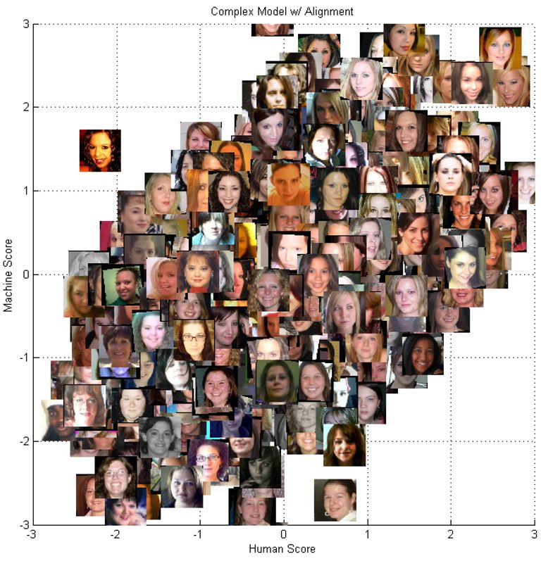
2      Predicting Facial Beauty without Landmarks

    The social science approach to this problem can be characterized by the
search for easily measurable and semantically meaningful features that are cor-
related with a human perception of beauty. In 1991, Alley and Cunningham
showed that averaging many aligned face images together produced an attrac-
tive face, but that many attractive faces were not at all average [3]. In 1994
Grammer and Thornhill showed that facial symmetry can be related to facial
attractiveness [4]. Since that time, the need for more complex feature represen-
tations has shifted research in this area to computer scientists.
    Most computer science approaches to this problem can be described as geo-
metric or landmark feature methods. A landmark feature is a manually selected
point on a human face that usually has some semantic meaning such as right
corner of mouth or center of left eye. The distances between these points and the
ratios between these distances are then extracted and used for classification using
some machine learning algorithm. While there are some methods of extracting
this information automatically [5] most previous work relies on a very accurate
set of dense manual labels, which are not currently available. Furthermore most
previous methods are evaluated on relatively small datasets with different evalu-
ation and ground truth methodologies. In 2001 Aarabi et al. built a classification
system based on 8 landmark ratios and evaluated the method on a dataset of
80 images rated on a scale of 1-4 [2]. In 2005 Eisenthal et al. assembled an en-
semble of features that included landmark distances and ratios, an indicator of
facial symmetry, skin smoothness, hair color, and the coefficients of an eigenface
decomposition [6]. Their method was evaluated on two datasets of 92 images
each with ratings 1-7. Kagian et al. later improved upon their method using an
improved feature selection method [7].
    Most recently Guo and Sim have explored the related problem of automatic
makeup application [8], which uses an example to transfer a style of makeup to
a new face.
    While all of the above methods produce respectable results for their respec-
tive data, they share a common set of flaws. Their datasets are very small and
usually restricted to a very small and meticulously prepared subset of the popu-
lation (e.g. uniform ethnicity, age, expression, pose and/or lighting conditions).
The images are studio-quality photos taken by professional photographers. As
another limitation, all these methods are not fully-automatic recognition sys-
tems, because they rely heavily on the accurate manual localization of landmark
features and often ignore the image itself once they are collected.
    We have attempted to solve the problem with fewer restrictions on the data
and a ground truth rating methodology that produces an accurate ranking of
the images in the data set. We have collected 2056 images of frontal female
faces aged 18-40 with few restrictions on ethnicity, lighting, pose, or expression.
Most of the face images are cropped from low-quality photos taken by cell-phone
cameras. The data size is 20 times larger the that of any previous study. Some
sorted examples can be found in figure 3, the ranking methodology is discussed
in section 2. Because of the heavy cost of labeling landmark features on such
a large data set, in this paper we solely focused on methodologies which do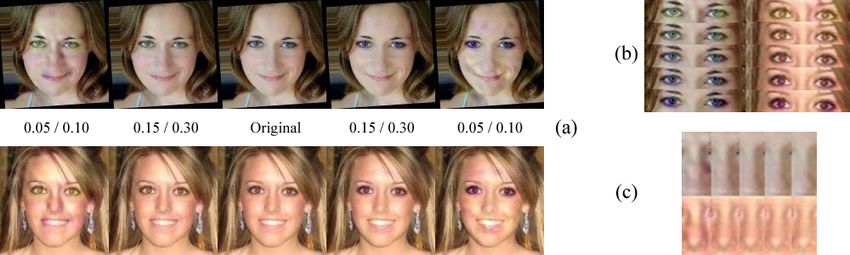
Predicting Facial Beauty without Landmarks           3

not require these features3 . Furthermore, although landmark features and ratios
appear to be correlated with facial attractiveness, it is yet unclear to what extent
human brains really use these features to form their notion of facial beauty. In
this paper we test the hypothesis if a biologically-inspired learning architecture
can achieve a near human-level performance on this particular task using a
large data set with few restrictions. The learning machine is an instance of the
Hubel-Wiesel model [9] which simulates the structure and functionality of visual
cortex systems, and consists of multiple layers of trainable feature extractors. In
section 3 we discuss discuss the details of the approach to predict female facial
attractiveness. In section 4.2 we present the experimental results. Interestingly,
we develop a novel way to visualize and interpret the learned black-box model,
which reveals some meaningful features highly relevant to beauty prediction and
complementary to previous findings.
    To summarize, we contribute to the field a method of quantifying and pre-
dicting female facial attractiveness using an automatically learned appearance
model (as opposed to a manual geometric model). A more realistic dataset has
been collected that is 20 times larger than any previously published work and has
far fewer restrictions. To the best of our knowledge, it is the first work to test if a
Hubel-Wiesel model can achieve a near human-level performance on the task of
scoring female facial attractiveness. We also provide a novel method of interpret-
ing the learned model and use it to present evidence for the existence of beautiful
features that go beyond the current averageness and symmetry hypotheses. We
believe that the work enriched the experiences of AI research toward building
generic intelligent systems.

2     Dataset and Ground Truth
In order to make a credible attack on this problem we require a large dataset
of high quality images labeled with a beauty score. As of the time of writing,
no such data are publicly available. However there does exist a popular website
HOTorNOT 4 with millions of images and billions of ratings. Users who submit
their photo to this site waive their privacy expectations and agree to have their
likeness criticized. Unfortunately the ratings that are associated with images in
this dataset were collected from images of people as opposed to faces, and are
not valid for the problem we are addressing. We have run face detection software
on a subset of images from this website and produced a dataset of 2056 images
and collected ratings of our own from 30 labelers.

2.1    Absolute vs. Pairwise Ratings
There are several kinds of ratings that can be collected for this task. The most
popular are absolute ratings where a user is presented with a single image and
3
    We also note that landmark feature methods fall outside the purview of computer
    vision as the original images may be discarded once the features are marked and
    ratings are collected.
4
    http://www.hotornot.com/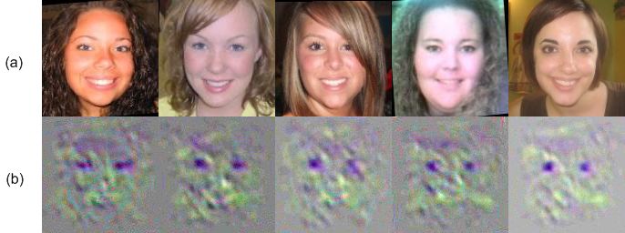
4        Predicting Facial Beauty without Landmarks

asked to give a score, typically between 1 and 10. Most previous work has used
some version of absolute ratings usually presented in the form of a Likert scale
[10] where the user is asked about the level of agreement with a statement. This
form of rating requires many users to rate each image such that a distribution
of ratings can be gathered and averaged to estimate the true score. This method
is less than ideal because each user will have a different system of rating images
and a user’s rating of one image may be affected by the rating given to the
previous image, among other things.
     Another method used in [11] was to ask a user to sort a collection of images
according to some criteria. This method is likely to give reliable ratings but it
is challenging for users to sort a large dataset since this requires considering all
the data at once.
     The final method is to present a user with pair of images and ask which is
more attractive. This method presents a user with a binary decision which we
have found can be made more quickly than an absolute rating. In section 2.3 we
show how to present an informative pair of images to a user in order to speed
up the process of ranking the images in a dataset. This is the method that we
have chosen to label our data.

2.2     Conversion to Global Absolute Score

Pairwise ratings are easy to collect, but in order to use them for building a
scoring system we need to convert the ratings into an absolute score for each
image. 5 To convert the scores from pairwise to absolute, we minimize a cost
function defined such that as many of the pairwise preferences as possible are
enforced and the scores lie within a specified range. Let s = {s1 , s2 , . . . , sN } be
the set of all scores assigned to images 1 to N . We formulate the problem into
minimizing the cost function:
                                      M
                                      X
                                                    −
                             J(s) =         φ(s+            T
                                               i − si ) + λs s                         (1)
                                      i=1

where (s+    −                                       th comparison and φ(d) is some
         i /si ) denotes the current scores of the i
cost function which penalizes images that have scores which disagree with one
of M pairwise preferences and λ is a regularization constant that controls the
range of final scores. We define φ(d) as an exponential cost function φ(d) = e−d .
However this function can be any monotonically increasing cost function such as
the hinge loss, which may be advisable in the presence of greater labeling noise.
A gradient descent approach is then used to minimize this cost function. This
iterative approach was chosen because as we receive new labels, we can quickly
update the scores without resolving the entire problem. Our implementation is
5
    One could alternatively train a model using image pairs and a siamese architecture
    such as in [12]. However a random cross validation split of the images would invalidate
    around half of the pairwise preferences.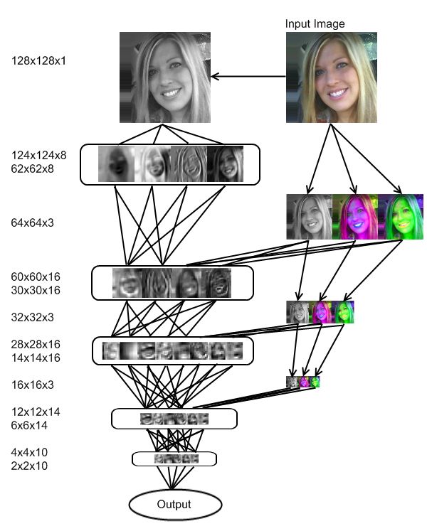
Predicting Facial Beauty without Landmarks              5

built on a web server which updates the scores in real time as new labels are
entered.
    We note that in our study we hypothesize that in a large sense people agree
on a consistent opinion on facial attractiveness, which is also the assumption
by most of the previous work. Each individual’s opinion can be varied due to
factors like culture, race, and education. In this paper we focus on learning the
common sense and leave further investigation on personal effects to future work.

2.3   Active learning

When our system is initialized, all images have a zero score and image pairs
are presented to users at random. However as many comparisons are made and
the scores begin to disperse, the efficacy of this strategy decays. The reason for
this is due in part to labeling noise. If two images with very different scores are
compared it is likely that the image with the higher score will be selected. If this
is the case, we learn almost nothing from this comparison. However if the user
accidentally clicks on the wrong image, this can have a very disruptive effect on
the accuracy of the ranking.

 Fig. 1. Simulation results for converting pairwise preferences to an absolute score.

   For this reason we use a relevance feedback approach to selecting image
pairs to present to the user. We first select an image at random with probability
inversely proportional to the number of ratings ri , it has received so far.

                                        (ri + )−1
                             p(Ii ) = PN                                           (2)
                                                    −1
                                       j=1 (rj + )

    We then select the next image with probability that decays with the distance
to first image score.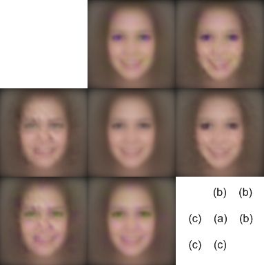
6       Predicting Facial Beauty without Landmarks

                                      exp (−(s1 − si )2 /σ 2 )
                       p(Ii |s1 ) = PN                                               (3)
                                                          2    2
                                     j=1 exp (−(s1 − sj ) /σ )

    Where σ 2 is the current variance of s. This approach is similar to the tour-
nament sort algorithm and has significantly reduced the number of pairwise
preferences needed to achieve a desired correlation of 0.9 (15k vs. 20k). Figure 1
shows the results of a simulation similar in size to our dataset. In this simulation
15% of the preferences were marked incorrectly to reflect the inherent noise in
collecting preference data.

3    Learning Methods

Fig. 2. An overview of the organization of our multiscale model. The first convolution is
only performed on the luminance channel. Downsampled versions of the original image
are fed back into the model at lower levels. Arrows represent downsampling, lines
represent convolution and the boxes represent downsampling with the max operator.
Feature dimensions are listed on the left (height x width x channels).

   Given a set of images and associated beauty scores, our task is to train a
regression model that can predict those scores. We adopt a predictive function
that models the relationship between an input image I and the output score s,
Predicting Facial Beauty without Landmarks 7
and learn the model in the following way
N
X
min (si − yi )2 + λwT w, s. t. yi = w> Φ(Ii ; θ) + b (4)
w,θ
i=1
where Ii is the raw-pixel of the i-th image represented by size 128x128 in YCbCr
colorspace, w is a D-dimensional weight vector, b is a scalar bias term, λ is a
positive scalar fixed to be 0.01 in our experiments. As a main difference from the
previous work, here we use Φ(·) to directly operate on raw pixels I for extracting
visual features, and its parameters θ are automatically learned from data with
no manual efforts. In our study we investigated the following special cases of the
model, whose differences are the definition of Φ(I; θ):
– Eigenface Approach: The method has been used for facial beauty prediction
by [6], perhaps the only attempt so far requiring no manual landmark fea-
tures. The method is as follows. We first run singular value decomposition
(SVD) on the input training data [I1 , . . . , IN ] to obtain its rank D decomposi-
tion UΣV> , and then set θ = U as a set of linear filters to operate on images
so that Φ(Ii ; θ) = U> Ii . We tried various D among {10, 20, 50, 100, 200} and
found that D = 100 gave the best performance.
– Single Layer Model: In contrast to Eigenface that uses global filters of re-
ceptive field 128 × 128, this model consists of 48 local 9 × 9 linear filters,
each followed by a non-linear logistic transformation. The filters convolute
over the whole image and produce 48 feature maps, which were then down
sampled by running max-operator within each non-overlapping 8 × 8 region
and thus reduced to 48 smaller 15 × 15 feature maps. The results serve as
the outputs of Φ(Ii ; θ).
– Two Layer Model: We further enrich the complexity of Φ(Ii ; θ) by adding
one more layer of feature extraction. In more details, in the first layer the
model employs separate 16 9×9 filters on the luminance channel, and 8 5×5
filters on a down-sampled chrominance channel; in the second layer, 24 5 × 5
filters are connected to the output of the previous layer, followed by max
down-sampling by a factor of 4.
– Multiscale Model: The model is similar to the single-layer model, but with
3 additional convolution/downsampling layers. A diagram of this model can
be found in figure 2. This model has 2974 tunable parameters6 .
In each of our models, every element of each filters is a learnable parameter (e.g.
if our first layer has 8 5x5 filters, then there will be 200 tunable parameters in
that layer). As we can see, these models represent a family of architectures with
gradually increased complexities: from linear to nonlinear, from single-layer to
multi-layer, from global to local, and from course to fine feature extractions. In
particular, the employed max operator makes the architecture more local- and
6
Note that this an order of magnitude less than the model trained for the task of face
verification in [12]8 Predicting Facial Beauty without Landmarks
partially scale-invariant, which is particularly useful in our case to handle the
diversity of natural facial photos. The architectures can all be seen as a form of
convolutional neural network [13] [12] that realize the well-known Hubel-Wiesel
model [14] inspired by the structure and functionalities of the visual cortex.
These systems were trained using stochastic gradient descent with a quadratic
loss function. Optimal performance on the test set was usually found within a
few hundred iterations, models with fewer parameters tend to converge faster
both in iterations and computation time. We have tested many models with
varying detailed configurations, and found in general that the number and size
of filters are not crucial but the number of layers are more important — Φ(Ii ; θ)
containing 4 layers of feature extraction generally outperformed the counterparts
with fewer layers.
4 Empirical Study
4.1 Prediction Results
A full and complete comparison with previous work would be challenging both to
perform and interpret. Most of the previous methods that have been successful
rely on many manually marked landmark features, the distances between them,
the ratios between those distances, and other hand crafted features. Manually
labeling every image in our dataset by hand would be very costly so we will only
compare with methods which do not require landmark features. As of the time
of publication, the only such method is the eigenface approach used in [6].
We compare the four learning methods described in Section 3 based on the
2056 female face images and the absolute scores computed from pair-wise com-
parisons. For each method, we investigate its performance on faces with and
without face alignment. We perform alignment using the unsupervised method
proposed in [15]. This approach is advantageous because it requires no manual
annotation. In all the experiments, we fixed the training set to be 1028 randomly
chosen images and used the remaining 1028 images for test.
Pearson’s correlation coefficient is used to evaluate the alignment between
the machine generated score and the human absolute score on the test data.
Table 1 shows a comparison between the four methods – eigenface, single layer,
two layer and multiscale models. We can see a significant improvement in the
performance with alignment for the eigenface approach and a slight improve-
ment for the hierarchal models. This discrepancy is likely due to the translation
invariance that is introduced by the local filtering and down sampling with the
max operator over multiple levels, as was first observed by [13]. Another obser-
vation is, with more layers being used, the performance improves. We note that
eigenface produced a correlation score 0.40 in [6] on 92 studio quality photos of
females with similar ages and the same ethnicity origins, but resulted very poor
accuracy in our experiments. This shows that the large variability of our data
significantly increased the difficulty of appearance-based approaches.
Though the Pearson’s correlation provides a quantitative evaluation on how
close the machine generated scores are to the human scores, it lacks of intuitivePredicting Facial Beauty without Landmarks 9
Method Correlation Correlation
w/o alignment w/ alignment
Eigenface 0.134 0.180
Single Layer Model 0.403 0.417
Two Layer Model 0.405 0.438
Multiscale Model 0.425 0.458
Table 1. Correlation score of different methods.
sense about this closeness. In figure 4 we show a scatter plot of the actual and
predicted scores for the multiscale model on the aligned test images. This plot
shows both the correlation found with our method and the variability in our data.
One way to look at the results is that, if without knowing the labels of axes, it
is quite difficult to tell which dimension is by human and which by machine. We
highly suggest readers to try such a test7 on figure 4 with an enlarged display.
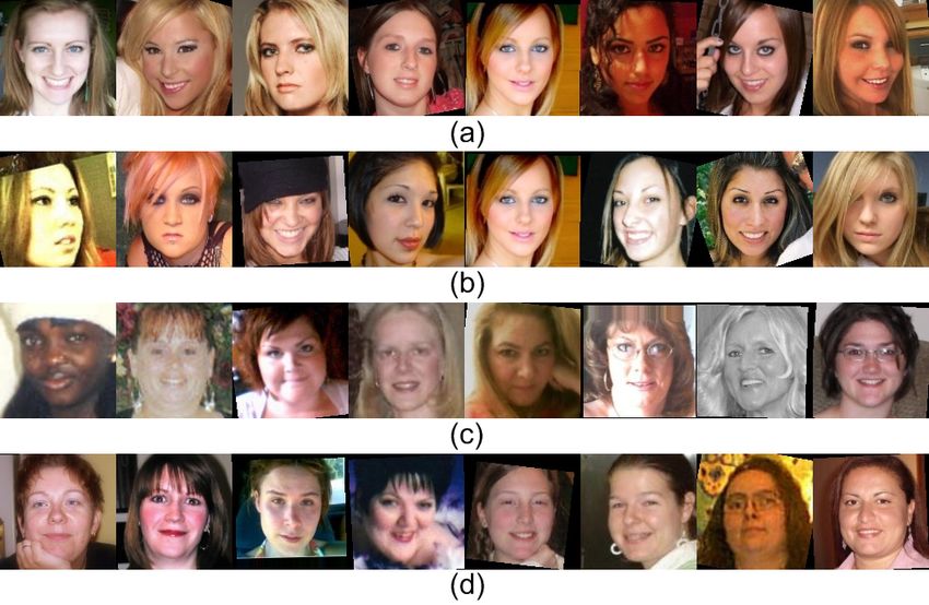
Figure 3 shows the top and bottom eight images according the humans and
the machine. Note that at the ground truth for our training was generated with
around 104 pairwise preferences, which is not sufficient to rank the data with
complete accuracy. However, the notion of complete accuracy is something that
can only be achieved for a single user, as no two people have the same exact
preferences.
4.2 What Does the Model Learn?
With so much variability it is difficult to determine what features are being used
for prediction. In this section we discuss a method of identifying these features
to better understand the learned models. One of the classic criticisms of the hi-
erarchical model and neural networks in general, is the black box problem. That
is, what features are we using and why are they relevant? This is typically ad-
dressed by presenting the convolution filters and noting their similarity to edge
detectors (e.g. gabor filters). This was interesting the first time it was presented,
but by now everyone in the community knows that edges are important for al-
most every vision task. We attempt to address this issue using a logical extension
to the backpropagation algorithm.
Backpropagation, the most fundamental tasks in training a neural network,
is where the gradient of the final error function is propagated back through each
layer in a network so that the gradient of each weight can be calculated w.r.t. the
final error function. When a neural network is trained, the training input and
associated labels are fixed, and the weights are iteratively optimized to reduce
the error between the prediction and the true label.
We propose the dual problem. Given a trained neural network, fix the weights,
set the gradient of the prediction to a fixed value and backpropagate the gradient
all the way through the network to the input image. This gives the derivative
7
Whether or not this constitutes a valid Turning test is left up to the reader.10 Predicting Facial Beauty without Landmarks
Fig. 3. The top (a/b) and bottom (c/d) eight images from our dataset according to
human ratings (a/c) and machine predictions (b/d).
of the image w.r.t. the concept the network was trained with. This information
is useful for several reasons. Most importantly, it indicates the regions of the
original image that are most relevant to the task at hand. Additionally, the sign
of the gradient indicates whether increasing the value of a particular pixel will
increase or decrease the network output, meaning we can perform a gradient
descent optimization on the original image.
Semantic Gradient Descent A regularized cost function w.r.t. a desired score
(s(d) ) and the corresponding gradient descent update can be written as:
J(It ) = φ(st − s(d) ) + λφ(It − I0 ) (5)
and
∂It
It+1 = It − ω + λ(It − I0 ) (6)
∂s
In our implementation we use φ(x) = x2 and use different values of λ for the
luminance and chrominance color channels.
The Derivative of Beauty The most pressing question is, What does the
derivative of beauty look like? Figure 5 shows several example images and their
respective gradients with respect to beauty for the multiscale model trained onPredicting Facial Beauty without Landmarks 11 Fig. 4. A Scatter plot showing actual and predicted scores with the corresponding faces. Fig. 5. Several faces (a) with their beauty derivative (b). These images are averaged over 10 gradient descent iterations and scaled in the colorspace for visibility.
12      Predicting Facial Beauty without Landmarks

aligned images. This clearly shows that the most important feature in this model
is the darkness and color of the eyes.
    The gradient descent approach can be used both to beautify and beastify the
original image. If we vary the regularization parameters and change the sign of
the derivative, we can visualize the image manifold induced by the optimization.
Figure 6 shows how specific features are modified as the regularization is relaxed.
    This shows most important features being used to predict beauty and concurs
with some human observations about the data and beauty in general.
    The first observation is that women often wear dark eye makeup to accentuate
their eyes. This makeup often has a dark blue or purple tint. We can see this
reflected on the extremes of figure 6 (c). In figure 6 (b), the eyes on the bottom
are dark blue/purple tint while the eyes on the top are bright with a yellow/green
tint.
    The second observation is that large noses are generally not very attractive.
If we again look at the extremes of figure 6 (c) we can see that the edges around
the nose on the right side have been smoothed, while the same edges on the left
side have been accentuated.

Fig. 6. The manifold of beauty for two images. (a) From left (beast) to right (beauty)
we can see how the regularization term (λY /λC ) controls the amount of modification.
Specific features from (a): Eyes (b) and Noses (c).

    The final observation is that a bright smile is attractive. Unfortunately the
large amount of variation in facial expressions and mouth position in our training
data leads to artifacts in these regions such as in the the extremes of figure 6.
However when we apply these modifications to the average image in figure 7, we
can see a change in the perceived expression.

Beautiful Features One of the early observations in the study of facial beauty
was that averaged faces are attractive [3]. This is known as the averageness hy-
pothesis. The average face from the dataset, presented in figure 7, has a score
of 0.026. The scores returned by the proposed model are all zero mean, indicat-
ing that the average face is only of average attractiveness. This would seem to
contradict the averageness hypothesis, however since the dataset presented here
Predicting Facial Beauty without Landmarks 13
Fig. 7. The average face image (a), beautified images (b) and beastified images (c).
The x axis represents changes in the luminance channel, while the y axis represents
changes in the chrominance channels.
was collected from a pool of user submitted photos, it does not represent a truly
random sampling of female faces (i.e. it may have a positive bias).
As of the time of publication, averageness, symmetry, and face geometry are
the only definable features that have been shown to be correlated with facial
attractiveness. This paper presents evidence that many of the cosmetic products
used by women to darken their eyes and hide lines and wrinkles are in fact
attractive features.
5 Conclusion
We have presented a method of both quantifying and predicting female facial
beauty using a hierarchical feed-forward model. Our method does not require
landmark features which makes it complimentary to the traditional geometric
approach [2] [16] [6] [7] [17] when the problem of accurately estimating landmark
feature locations is solved. The system has been evaluated on a more realistic
dataset that is an order of magnitude larger than any previously published re-
sults. It has been shown that in addition to achieving a statistically significant
level of correlation with human ratings, the features extracted have semantic
meaning. We believe that the work enriches the experience of AI research to-
ward building generic intelligent systems. Our future work is to improve the
prediction for this problem and to extend our work to cover the other half of the
human population.14 Predicting Facial Beauty without Landmarks
References
1. Cross, J., Cross, J.: Age, Sex, Race, and the Perception of Facial Beauty. Devel-
opmental Psychology 5 (1971) 433–439
2. Aarabi, P., Hughes, D., Mohajer, K., Emami, M.: The automatic measurement of
facial beauty. Systems, Man, and Cybernetics, IEEE International Conference on
4 (2001)
3. Alley, T., Cunningham, M.: Averaged faces are attractive, but very attractive faces
are not average. Psychological Science 2 (1991) 123–125
4. Grammer, K., Thornhill, R.: Human (Homo sapiens) facial attractiveness and
sexual selection: the role of symmetry and averageness. J Comp Psychol 108
(1994) 233–42
5. Zhou, Y., Gu, L., Zhang, H.: Bayesian tangent shape model: estimating shape and
pose parameters via Bayesian inference. Computer Vision and Pattern Recognition,
IEEE Computer Society Conference on 1 (2003)
6. Eisenthal, Y., Dror, G., Ruppin, E.: Facial Attractiveness: Beauty and the Machine
(2005)
7. Kagian, A., Dror, G., Leyvand, T., Cohen-Or, D., Ruppin, E.: A Humanlike Predic-
tor of Facial Attractiveness. Advances in Neural Information Processing Systems
(2005) 649–656
8. Guo, D., Sim, T.: Digital face makeup by example. Computer Vision and Pattern
Recognition, IEEE Computer Society Conference on (2009)
9. Hubel, D., Wiesel, T.: Receptive fields and functional architecture of monkey
striate cortex. The Journal of Physiology 195 (1968) 215–243
10. Likert, R.: Technique for the measurement of attitudes. Arch. Psychol 22 (1932)
55
11. Oliva, A., Torralba, A.: Modeling the Shape of the Scene: A Holistic Representation
of the Spatial Envelope. International Journal of Computer Vision 42 (2001) 145–
175
12. Chopra, S., Hadsell, R., LeCun, Y.: Learning a similarity metric discriminatively,
with application to face verification. Computer Vision and Pattern Recognition,
IEEE Computer Society Conference on 1 (2005)
13. Fukushima, K.: Neocognitron: A hierarchical neural network capable of visual
pattern recognition. Neural Networks 1 (1988) 119–130
14. Hubel, D., Wiesel, T.: Receptive fields, binocular interaction and functional archi-
tecture in the cats visual cortex. Journal of Physiology 160 (1962) 106–154
15. Huang, G., Jain, V., Amherst, M., Learned-Miller, E.: Unsupervised Joint Align-
ment of Complex Images. Computer Vision, IEEE International Conference on
(2007)
16. Gunes, H., Piccardi, M., Jan, T.: Comparative beauty classification for pre-surgery
planning. Systems, Man and Cybernetics, IEEE International Conference on 3
(2004)
17. Joy, K., Primeaux, D.: A Comparison of Two Contributive Analysis Methods Ap-
plied to an ANN Modeling Facial Attractiveness. Software Engineering Research,
Management and Applications, International Conference on (2006) 82–86You can also read