Mapping Missing Population in Rural India: A Deep Learning Approach with Satellite Imagery - aies-conference.com
←
→
Page content transcription
If your browser does not render page correctly, please read the page content below

Mapping Missing Population in Rural India:
                          A Deep Learning Approach with Satellite Imagery
       Wenjie Hu,3 Jay Harshadbhai Patel,1 Zoe-Alanah Robert,1 Paul Novosad,4 Samuel Asher5
                  Zhongyi Tang,6 Marshall Burke,2 David Lobell,2 Stefano Ermon1
 1
     Department of Computer Science, Stanford University, {jayhp9, zrobert7}@alumni.stanford.edu, ermon@cs.stanford.edu
                 2
                   Department of Earth System Science, Stanford University, {mburke, dlobell}@stanford.edu
                         3
                           Department of Statistics, Stanford University, huwenjie@alumni.stanford.edu
                         4
                           Department of Economics, Dartmouth College, paul.novosad@dartmouth.edu
                              5
                                Development Research Group, World Bank, sasher@worldbank.org
                       6
                         Stanford Institute for Economic Policy Research (SIEPR), zztang@stanford.edu

                           Abstract                                   However, creating a population map with high accuracy
                                                                   and high resolution is a challenging problem. Tradition-
  Millions of people worldwide are absent from their country’s
  census. Accurate, current, and granular population metrics       ally, it is done by performing a high-cost national census.
  are critical to improving government allocation of resources,    The USAID Demographic and Health Survey (DHS) pro-
  to measuring disease control, to responding to natural disas-    gram performs surveys for developing countries typically
  ters, and to studying any aspect of human life in these com-     every 5 years, and each survey costs anywhere from 1.1
  munities. Satellite imagery can provide sufficient information   million to 9.7 million USD (Doupe et al. 2016). The cen-
  to build a population map without the cost and time of a gov-    sus surveys are even more expensive in developed countries
  ernment census. We present two Convolutional Neural Net-         like Europe, with a median cost of USD 5.57 per capita in
  work (CNN) architectures which efficiently and effectively       2010 (UN 2014). For some countries with financial diffi-
  combine satellite imagery inputs from multiple sources to ac-    culties or political instability, the census is carried out less
  curately predict the population density of a region. In this
                                                                   frequently, as few as once every few decades (UN 2016a;
  paper, we use satellite imagery from rural villages in India
  and population labels from the 2011 SECC census. Our best        2016b). Reliance on out-of-date population statistics can
  model achieves better performance than previous papers as        lead to significant errors if used for policy making or re-
  well as LandScan, a community standard for global popula-        source allocation.
  tion distribution.                                                  In this project, we aim to predict the population density of
                                                                   rural villages of India from high-resolution satellite imagery
                                                                   by utilizing Convolutional Neural Network (CNN) models.
                     1    Introduction                             With the availability of high-frequency satellite images, we
In 2015, the United Nations set forth seventeen objectives         can predict population density every few days, saving the
to “end poverty, protect the planet and ensure prosperity for      costs of on-site census surveys and avoiding the inaccuracies
all” known as the Sustainable Development Goals (SGD)              caused by the infrequency of census surveys. We demon-
(UN 2015). To monitor progress and ultimately achieve              strate state-of-the-art prediction performance in villages of
these objectives, accurate population statistics are essential.    all states in India. By using satellite images with 10-30 me-
It is estimated that currently 300-350 million people world-       ter resolution, our best models can predict aggregated village
wide are not included in their countrys official population        population in one Subdistrict (akin to a US county) with R2
document, which hurts the measurement of SGD progress              of 0.93, and individual village log2 population density with
(Carr-Hill 2013). The ability to quickly and cost-effectively      R2 of 0.44.
produce an accurate population map for a country has a mul-
titude of benefits. Those missing populations are more likely                          2   Related Work
to be marginalized communities which already do not re-
ceive sufficient resources from the government (UNICEF             2.1   Traditional Methods
2016). An accurate population distribution is an essential         Traditionally, population mapping is divided into two ap-
basis for socioeconomic statistics, such as food, water, and       proaches, population projection and population disaggre-
energy demand in different regions of a country, which in-         gation. Population projection predicts the future or current
fluence the policy-making and spending decisions of its gov-       population of a region based on historical data. For most
ernment. Additionally, during natural disasters such as earth-     cases, simple linear regression is sufficient for the projec-
quakes and floods, an accurate population map can help or-         tion (Smith 1987). In more complex models, projections take
ganize rescue efforts more quickly and effectively. For re-        into consideration historic population data, birth rates, reg-
gions with high infectious disease rates, a fine-grained popu-     istered vehicles, etc (Long 1993). These models were used
lation map also helps to prevent the spread of infectious dis-     to project US county population in 5 years, which have very
eases to locations with dense population (Tatem et al. 2012;       high accuracy with R2 of 0.99. However, they don’t provide
Hay et al. 2005).                                                  information about the population distribution within each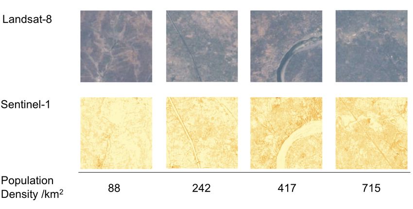
county.                                                          evenly to the areas covered by human-made structures, and
                                                                 create population maps with ∼30 meter resolution for 18
                                                                 countries, not including India (Tiecke et al. 2017).
                                                                    Instead of disaggregation based on population estimates
                                                                 from census surveys, some CNN models are trained to es-
                                                                 timate population directly from satellite imagery inputs.
                                                                 Doupe et al. combined Landsat-7 satellite imagery with
                                                                 (DMSP/OLS) nighttime lights as CNN input, and predicted
                                                                 the log normalized population density for an area of 8km2
                                                                 (called LL-raw), where the ground-truth label was average
                                                                 population density of Sublocation (akin to a US county). The
                                                                 outputs were then converted into weights and used to cre-
                                                                 ate a weighted population density surface across the coun-
                                                                 try with a single known total population (LL-distributed).
                                                                 The model was trained with 2002 Tanzanian Enumeration
                                                                 Areas and tested with 2009 Kenya Sublocations. During the
                                                                 test phase, the estimated population densities were averaged
Figure 1: Population disaggregation visualization for World-     at the Sublocation level, and then compared to other meth-
Pop(A,D), GRUMP (B,E), LandScan (C,F). The upper 3               ods. The results show that LL-raw has better accuracy than
figures show a northeast region of Guinea along the Niger        GRUMP and GWP estimates, and that LL-distributed out-
River; the lower 3 figures show the region around the largest    performs a random forest model by 177% on RMSE (Doupe
city of Tanzania, Dar es Salaam. (WorldPop 2018)                 et al. 2016).
                                                                    Robinson, Hohman, and Dilkina in 2017 adopted a sim-
                                                                 ilar CNN approach to (Doupe et al. 2016), but changed the
   The more challenging task is population disaggregation,       model output from regression to classification of the power
which involves estimating the population distribution of a       level of population. The model only uses Landsat imagery
region given the total population. The most basic method         as input, and predicts population in the US with US Cen-
is areal weighting/interpolation, which assumes a uniform        sus Summary Grids data as ground-truth labels. The study
distribution across the region with a single population value    divided the country into 15 regions, and trained an individ-
(Goodchild, Anselin, and Deichmann 1993). The Gridded            ual model for each region. The raw output feature vectors of
Population of the World (GPW) uses areal weighting with          the CNN model were first converted into population values
a resolution of 30 arc-seconds (approximately 1 km at            for each input image, and then summed at the county level
the equator) (CIESIN 2010). There are also many tools            to produce CONVRAW. The outputs of the CNN were also
which implement a weighted surface for estimating a pop-         fed into a second layer gradient boosting model to get an
ulation’s distribution, a technique otherwise called dasy-       improved population estimate for each county called CON-
metric weighting (Robinson, Hohman, and Dilkina 2017).           VAUG, where the census county population was used as la-
The Global Rural Urban Mapping Project (GRUMP) uses              bels. The results of CNN models achieved more than 0.9 R2
nightlight imagery to add urban and rural boundaries to          against the ground truth, but still cannot perform better than
GPW (Schneider, Friedl, and Potere 2009). LandScan esti-         the US government estimate based on historical census data
mates the weighted surface (with 30 arc-seconds resolution)      (Robinson, Hohman, and Dilkina 2017).
for population distribution based on land cover, roads, slope,
urban areas, village locations (ORNL 2011). AfriPop, Asi-
aPop, and AmeriPop are similar but for region-specific pop-                               3    Data
ulation disaggregation calculations, and they are combined       3.1   Population Dataset
in the 2013 WorldPop project (Worldpop 2013), which has a
                                                                 Our ground-truth Indian population dataset comes from a
higher resolution of 100 meters. These disaggregation meth-
                                                                 census survey Socio-Economic Caste Census in the year
ods are compared visually in Figure 1.
                                                                 2011 (SECC 2011). It includes more than 500,000 rural
                                                                 villages, covering 32 states, 619 districts, and 5724 sub-
2.2   Machine Learning Methods                                   districts. It also provides the area of each surveyed village.
In addition to the above traditional GIS approach, machine       Figure 2 shows the distribution of areas follows a power law.
learning algorithms have been proposed in recent years to        These areas are used to calculate population density for each
obtain better population disaggregation results. A random        village. Similar to previous papers, we log normalize pop-
forest approach was used to estimate the population at 100m      ulation density values with base 2, because most villages
resolution for Vietnam, Cambodia, and Kenya, using fea-          have small population density, and only a few have large
tures similar to LandScan (Stevens et al. 2015). The Face-       density. The original density input may cause the model to
book Connectivity Lab used a tailored CNN model to de-           have less ability to predict villages with higher population
tect man-made structures from satellite imagery with 0.5m        density. The distribution of villages density after log2 nor-
resolution, which achieved average precision of 0.95 and re-     malization is shown in Figure 3.
call of 0.91. They then redistributed the population in GPW         Inspecting the population datasets we observed some out-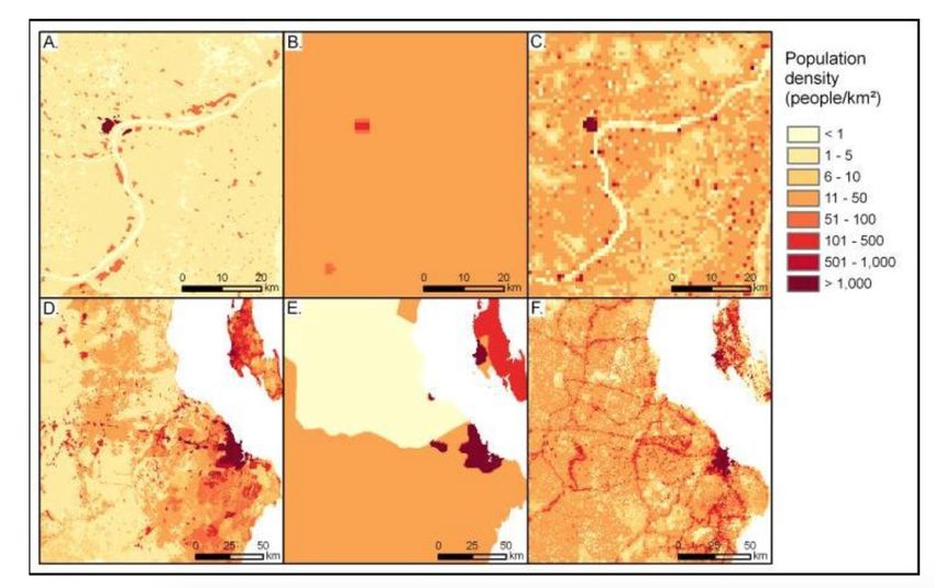
thereby capturing roads and roofs more accurately (due to
                                                                their higher reflectance than natural land) (ESA 2014). This
                                                                is a new dataset not used in the previously mentioned pa-
                                                                pers. Sentinel-1 images have 10-meter resolution, and the
                                                                raw channel values are converted to visualized RGB images
                                                                to match Landsat-8. Both sets of images are converted to
                                                                JPEG format from raw GeoTIFF files, which enables easy
                                                                visualization and compression. Figure 4 displays examples
                                                                of these images.

            Figure 2: Village area distribution.

                                                                Figure 4: Landsat-8 and Sentinel-1 imagery examples, with
                                                                corresponding ground truth population density from the sur-
                                                                vey.

                                                                   Since Landsat-8 and Sentinel-1 have different spatial res-
                                                                olutions, they are cropped to cover the same area. Based on
                                                                the village area distribution as shown in Figure 2, the cov-
                                                                ered area of images is determined to be 20.25 km2 (4.5km
                                                                × 4.5km), so that more than 95% of villages are contained
Figure 3: Village population density distribution after log2
                                                                within a single satellite image.
normalization.
                                                                3.3   Dataset Partition
lier values, such as a 100 km2 area with just one person. We    We split the dataset of ground-truth population (outputs) and
assume these are due to data collection and handling mis-       images (inputs) pairs into 70% training and 30% validation
takes, therefore we remove 1% of village data that had ex-      partitions. We took additional measures to avoid the over-
treme population density values to prevent the model train-     lap of training images with validation images, which may
ing from being affected by those outliers. More specifically,   affect the reliability of the validation split. Overlaps are very
villages with top 0.5% highest density and bottom 0.5% low-     likely because the total area of all satellite images (over 10
est density were removed from the datasets.                     million km2 ) we obtained is much larger than the total area
                                                                of India (about 3.3 million km2 ). To address this issue, we
3.2   Satellite Imagery                                         partition the data at the subdistrict level. We split all sub-
For each village, we prepare one image from each satellite      districts into 4007 training and 1717 validation subdistricts.
imagery source such that the village center is found at the     The training partition only has images of villages that be-
image center. The village population depends on its area but    long to training subdistricts, and similarly for the validation
our images have fixed size covering the same area, therefore    partition. However, it is still possible that images overlap
we use population density as the output. We obtained 2 sets     along the boundary of two adjacent subdistricts, contami-
of satellite imagery from 2011, the same year the survey was    nating the split. Thus, we remove additional images from the
conducted. The first set is from Landsat-8, an updated satel-   training partition. We say a pair of images overlap if the dis-
lite from Landsat-7 whose images are also used by papers        tance between their centers is closer than half of the height or
from Robinson, Hohman, and Dilkina in 2017 and Doupe et         width of the image (2.25km). Approximately an additional
al. in 2016 (USGS 2013). In contrast with previous papers       5% overlapping images are removed from the training parti-
which use most bands of Landsat, we use only Red, Green,        tion.
and Blue (RGB) bands. The resulting images show the tar-
get regions in the same colors that humans see, and have 30-                            4    Method
meter resolution. The second set is from Sentinel-1, a radar    We propose a deep learning approach that uses satellite im-
imaging satellite that measures ground surface reflectance,     ages as inputs to a Convolutional Neural Network (CNN)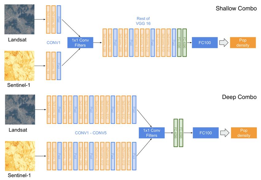
to predict population density. The ground-truth population         papers, which we are going to compare with. In short, the
data is used as the label to train the model. We start with        village level evaluation uses log2 population density values,
the VGG16 architecture (Simonyan and Zisserman 2014),              while subdistrict level evaluation uses real population num-
using as input either Landsat-8 or Sentinel-1 RGB images.          bers.
We use the implementation of VGG 16 from the TensorFlow               In terms of evaluation metrics, we compare different mod-
Slim Library. To adapt the model for a regression problem,         els mainly based on R2 and Pearson Correlation. R2 mea-
the model output size is set to be 1 for a single log2 popu-       sures how much true variance is captured by the model, and
lation value. Additionally, the loss function in the model is      attains a perfect value at 1. If a model makes constant aver-
changed to Mean Squared Error (MSE). Image inputs are re-          age predictions, it will have R2 score of 0. Pearson Corre-
sized to 224 × 224 × 3 (width × height × channels), and we         lation measures the linear correlation between the predicted
apply image augmentation including random cropping and             and true values, implying a total positive correlation when
flipping during training. The model weights are initialized        +1 and a total negative correlation when -1. We also use
with pre-trained weights from the ILSVRC-2010-CLS Ima-             other metrics to compare results with previous papers, such
geNet classification dataset, omitting the last (classification)   as MAPE (Mean Absolute Percentage Error), %RMSE (per-
layer.                                                             cent Root Mean Squared Error).
   To fully utilize multiple satellite image sources in this
study, we design two custom CNN architectures. The first           5.2   Baseline: LandScan
custom architecture, called Shallow Combo, is shown in             To establish a baseline comparison for this project, we com-
Figure 5. It is a modified version of VGG16 where Landsat          pared our ground truth population densities with those of
and Sentinel-1 images are input into the model separately          LandScan, which is considered a community standard for
as two branches. In each branch, two convolution layers and        global population distribution (ORNL 2011). LandScan is
one max pooling layer (CONV1 in VGG16) are applied to              a grid containing a numerical population estimate for every
each image. The two branches are then concatenated along           cell of size 30x30 arc-second in earth coordinates, which is
the channel dimension. 1 × 1 convolutions filters are ap-          around 1km on the equator (smaller at different latitudes).
plied to halve the number of channels after concatenation,         This estimate represents an average (over 24 hours), or am-
which fits the input shape of next convolutional layer. The        bient population distribution (not just sleeping location). For
rest of the VGG16 layers are applied to the merged branch.         a single village, we take a square of 30 arc-second cells
After the last fully connected layer of VGG16, one more            which most closely matches the villages area, as well as the
fully connected layer of size 100 is added to the network.         village latitude and longitude. The population density of the
The layer is lastly used to predict the output log2 popula-        village is calculated by dividing the LandScan population
tion density. During training, weights of all convolutional        estimates within the cells with the area covered by the cells.
layers and the first two fully connected layers are initialized       We use this method to obtain the LandScan estimate of
with pre-trained weights from the basic VGG16 architecture         population density for all villages in our validation dataset.
trained on ImageNet.                                               The evaluation results are shown as LandScan model in
   The second custom CNN called Deep Combo is an im-               Table 2. It has good performance in estimating aggregated
proved version of Shallow Combo, also shown in Figure              population on subdistrict level, but it doesn’t perform well
5. The branches of Landsat and Sentinel-1 are fed through          on per-village level. It is reasonable because LandScan is
all convolutional layers of VGG16, and concatenated along          a traditional population disaggregation method using only
the channel dimension before the first fully connected layer.      the general features on the maps, such as rivers, roads, land
The same 1 × 1 convolutions filters are applied to obtain the      cover types. It does not have fine-grained information as our
same input shape before the fully connected layer. ImageNet        models have from satellite imagery.
weights are also used for initialization until the second fully
connected layer.                                                   5.3   Single State Training
                                                                   Due to the large amount of data, we initially generate a
               5    Experimental results                           smaller dataset with villages in a single state, Gujarat. The
                                                                   small dataset contains around 13,000 villages, which al-
5.1   Evaluation Methods                                           lows us to compare different models quickly, and to tune
We evaluate each model on the validation set on two lev-           the hyper-parameters of the CNN models. We experiment
els: raw village level and aggregated subdistrict level. The       with different input sources and the different CNN architec-
raw village level predictions are per-village log2 population      tures described above. We train the basic VGG-16 separately
density estimates from the model, which are compared with          with Landsat-8 (L8) and Sentinel-1(S1) inputs. The L8 and
the ground-truth census population density of each village.        S1 inputs are also concatenated along the image channels
This raw evaluation represents the most fine-grained com-          and feed into VGG-16 as single input (S1L8-Concat). Fur-
parison possible in our dataset. At the aggregated subdistrict     thermore, Shallow Combo and Deep Combo architectures
level, the raw per-village density predictions are converted       are used to process two type of satellite images separately.
to the total village population using the village area from the    We use NVIDIA Tesla P100 GPU with 16G memory from
survey. The village populations within each subdistrict are        Google Compute Engine for training. It sets the limit of in-
aggregated to a total population for that subdistrict. Eval-       put batch size to 48 for the Deep Combo architecture, thus
uations at the aggregate levels are performed in previous          this batch size is also used for other models to ensure a
Figure 5: Custom CNN architecture Shallow Combo (upper) and Deep Combo (lower)
fair comparison. With several iterations, the optimal hyper- tectures have significantly better performance. These results
parameters are found as follows: learning rate: 10−5 , expo- indicate that when using inputs from different sources, the
nential learning decay rate: 10−1 , weight decay: 5x10⁻³ , CNN model needs to process them separately to extract their
dropout: 0.8. semantic features, so that useful information from both sides
can be utilized.
Table 1: Evaluation of Single State Training 5.4 All States Training
Village level Subdistrict level After training on a single state, we move on to train on
Model around 350,000 villages in all 32 states in India. L8, S1,
R2 Pearson R2 Pearson
Shallow Combo and Deep Combo are trained respectively
L8 0.111 0.443 0.597 0.775
with the same hyper-parameters found when training in
S1 0.120 0.425 0.701 0.839
the single state case. The evaluation results are summa-
L8S1-Concat 0.111 0.472 0.305 0.764
rized in Table 2. With more data provided, all the models
Shallow Combo 0.200 0.488 0.739 0.889
show significant improvements. All models exceed the per-
Deep Combo 0.167 0.489 0.772 0.921
formance of the LandScan baseline. Shallow Combo and
Deep Combo models still outperform the basic VGG-16
The evaluations of the above 5 models are shown in Table models with a single image source. By comparing between
1. In general, the models have lower accuracies when pre- two custom architectures, Shallow Combo has better per-
dicting per-village level population densities, but the accu- formance on predicting population on a single village, while
racy significantly improves when the individual predictions Deep Combo captures more general information in the re-
are aggregated for the subdistrict level evaluation. The S1 gion and has better accuracy when predicting aggregated
model has better performance than the L8 model, possibly population at the subdistrict level.
due to its high resolution as well as that measuring ground
reflectance by radar is more effective. However, simply con- 5.5 Comparison with Prior Works
catenating L8 and S1 inputs in L8S1-Concat does not lead In this section, we compare our models with others from
to further improvements, resulting in performance slightly prior studies, using aggregated evaluation metrics. Table 3
worse than using S1 alone. This is likely due to training dif- summarizes the reported accuracies from the papers from
ficulties when using a combination of L8 and S1 images. Doupe et al. in 2016 with study area in Kenya, and from
In contrast, our Shallow Combo and Deep Combo archi- Robinson, Hohman, and Dilkina in 2017 with study area in• Additional Sentinel-1 satellite imagery that provides more
Table 2: Evaluation of All States Training information on human settlements.
Village level Subdistrict level
Model • Custom Shallow Combo and Deep Combo CNN archi-
R2 Pearson R2 Pearson
tectures that better utilize different imagery sources.
L8 0.346 0.596 0.838 0.919
S1 0.327 0.597 0.890 0.944 • A larger and fine-grained dataset for CNN training.
Shallow Combo 0.438 0.663 0.906 0.954 • Better computational resources that enable larger image
Deep Combo 0.389 0.645 0.931 0.965 input size and batch size.
LandScan -0.553 0.476 0.835 0.928
CONVRAW 0.322 0.592 0.850 0.937 Our study largely achieves the initial goal of producing ac-
curate population estimates enabling population mapping
directly from satellite imagery, especially for rural areas.
The results show that population prediction at a relatively
the United States. Since we do not use subdistrict level pop-
coarse scale (such as district or subdistrict level) is quite
ulation for either training or prediction improvement, to en-
accurate, while prediction at the village level directly from
sure the fair comparison, we compare to the models in the
satellite imagery remains challenging. However, our village
papers also without the assistance of additional data from
level predictions already have significantly better perfor-
the aggregated level, namely LL-raw from Doupe’s paper
mance than traditional methods such as LandScan, and may
and CONVRAW from Robinson’s paper. Comparing with
still have room for improvement if images with higher res-
Robinson’s paper shows that even though we use a smaller
olution are available. Our population mapping models are
(average) aggregation area in India, we still achieve sig-
likely useful for assisting governments in better providing
nificantly better R2 and MAPE. The aggregation area in
for their citizens, improving resource allocation in natural
Doupe’s study is even smaller, but their model also has much
disasters, aiding in infectious disease tracking, and reducing
higher errors compared to ours.
bias in progress measurement for the United Nations SDGs.
Table 3: Comparison with Prior Works 7 Appendix
Paper Ours Robinson Doupe we visualize the population mapping of different models in
2017 2016 districts of India, the higher administrative level than sub-
Study area India US Kenya district, as shown in Figure 6. It includes 533 districts that
Aggr. area 424 km2 2584 km2 88 km2 contain evaluation results from 1717 validation subdistricts.
Model Deep Combo CONVRAW LL-Raw The visualization includes our Deep Combo and Shallow
R2 0.931 0.910 - Combo model predictions compared with ground-truth pop-
MAPE 21.5 73.8 - ulation density distribution across districts in India. It also
%RMSE 24.3 - 145.43 compares the prediction errors of the two models with those
of the baseline LandScan and CONVRAW model from
(Robinson, Hohman, and Dilkina 2017). Overall, both Deep
However, it is difficult to compare models trained and Combo and Shallow Combo models map the rural vil-
tested across different countries. To address this problem, we lage population of India very close to the true distribution.
use the same methods from (Robinson, Hohman, and Dilk- The prediction errors map further reveals that Deep Combo
ina 2017) and apply them to our India study area. Specifi- has better performance on high level aggregation than other
cally, we trained a classification model using a single Land- models, while LandScan tends to underestimate the popu-
sat input. The categorical outputs of the CNN are in the bins lation and CONVRAW tends to overestimate.
of log2 population density values for each Indian village.
Following its CONVRAW approach, we convert the pre-
dicted class to population density, and aggregate the pop- 8 Acknowledgments
ulation at the subdistrict level. The predictions are still not This work was supported by Data for Development Initia-
as good as most of our models, which are shown as CON- tive at the Stanford Center on Global Poverty and Devel-
VRAW in Table 2. Its performance is close to our L8 model, opment. All data in this work was processed and shared by
which differs from it by using regression instead of classifi- Paul Novosad (Dartmouth College) and Sam Asher (World
cation. The comparison shows the regression model is better Bank).
at predicting fine-grained population while classification is
better for aggregate predictions. References
6 Conclusion Carr-Hill, R. 2013. Missing millions and measuring devel-
opment progress. World Development 46:30–44.
The results of our CNN models on the population density
prediction directly from satellite imagery are very promis- CIESIN. 2010. Gridded population of the world (gpw), v4:
ing. We see a higher accuracy than previous methods on Population count grid.
both per-image raw level and aggregated region level. We Doupe, P.; Bruzelius, E.; Faghmous, J.; and Ruchman, S. G.
attribute the success to the following reasons: 2016. Equitable development through deep learning: TheFigure 6: Population mapping visualization on the validation dataset. The upper row shows the population predictions of Deep
Combo and Shallow Combo model compared to the ground-truth values. The lower row shows the prediction errors of Deep
Combo and Shallow Combo compared with the baseline LandScan, and CONVRAW model from previous paper (Robinson,
Hohman, and Dilkina 2017). The grey areas are the regions with no validation data.
case of sub-national population density estimation. In Pro- county population projections. Journal of the American Sta-
ceedings of the 7th Annual Symposium on Computing for tistical Association.
Development, 6. ACM. Stevens, F. R.; Gaughan, A. E.; Linard, C.; and Tatem, A. J.
ESA. 2014. Sentinel-1 - missions. 2015. Disaggregating census data for population mapping
using random forests with remotely-sensed and ancillary
Goodchild, M. F.; Anselin, L.; and Deichmann, U. 1993. data. PloS one 10(2):e0107042.
A framework for the areal interpo- lation of socioeconomic
data. Environment and planning. Tatem, A. J.; Adamo, S.; Bharti, N.; Burgert, C. R.; Castro,
M.; Dorelien, A.; Fink, G.; Linard, C.; John, M.; Montana,
Hay, S. I.; Noor, A. M.; Nelson, A.; and Tatem, A. J. 2005. L.; Montgomery, M. R.; Nelson, A.; Noor, A. M.; Pindolia,
The accuracy of human population maps for public health D.; Yetman, G.; and Balk, D. 2012. Mapping populations
application. Trop Med Int Health 10(10):1073–1086. at risk: improving spatial demographic data for infectious
ORNL. 2011. Landscan - oak ridge national laboratory. disease modeling and metric derivation. Population Health
Metrics 10(1):8.
Robinson, C.; Hohman, F.; and Dilkina, B. 2017. A deep
learning approach for population estimation from satellite Tiecke, T. G.; Liu, X.; Zhang, A.; Gros, A.; Li, N.; Yetman,
imagery. CoRR abs/1708.09086. G.; Kilic, T.; Murray, S.; Blankespoor, B.; Prydz, E. B.; and
Dang, H.-A. H. 2017. Mapping the world population one
Schneider, A.; Friedl, M. A.; and Potere, D. 2009. A new building at a time. ArXiv e-prints.
map of global urban extent from modis satellite data. Envi-
UN. 2014. Measuring population and housing: practices of
ronmental Research Letters.
the unece countries in the 2010 round of censuses. Technical
SECC. 2011. Socio economic and caste census-2011. report, United Nations.
Simonyan, K., and Zisserman, A. 2014. Very deep convo- UN. 2015. Sustainable development goals.
lutional networks for large-scale image recognition. arXiv UN. 2016a. Census dates for all countries.
preprint arXiv:1409.1556. UN. 2016b. Census reaches vulnerable women and girls in
Smith, S. K. 1987. Tests of forecast accuracy and bias for a remote area of myanmar for the very first time.UNICEF. 2016. The state of the world’s children 2012: A fair chance for every child. Technical report, UNICEF. USGS. 2013. Landsat missions. Worldpop. 2013. Worldpop - what is worldpop? WorldPop. 2018. Worldpop spatial dataset methods - www.worldpop.org.uk/data/methods/.
You can also read