Deep Sea Robotic Imaging Simulator
←
→
Page content transcription
If your browser does not render page correctly, please read the page content below
Deep Sea Robotic Imaging Simulator

                                         Yifan Song1 , David Nakath1 , Mengkun She1 , Furkan Elibol1 , and Kevin Köser1

                                                                 Oceanic Machine Vision,
                                                GEOMAR Helmholtz Centre for Ocean Research Kiel, Kiel, Germany
                                                              https://www.geomar.de/en/omv
                                                   {ysong; dnakath; mshe; felibol; kkoeser}@geomar.de
arXiv:2006.15398v2 [cs.CV] 12 Oct 2020

                                               Abstract. Nowadays underwater vision systems are being widely ap-
                                               plied in ocean research. However, the largest portion of the ocean - the
                                               deep sea - still remains mostly unexplored. Only relatively few image
                                               sets have been taken from the deep sea due to the physical limitations
                                               caused by technical challenges and enormous costs. Deep sea images are
                                               very different from the images taken in shallow waters and this area
                                               did not get much attention from the community. The shortage of deep
                                               sea images and the corresponding ground truth data for evaluation and
                                               training is becoming a bottleneck for the development of underwater
                                               computer vision methods. Thus, this paper presents a physical model-
                                               based image simulation solution, which uses an in-air texture and depth
                                               information as inputs, to generate underwater image sequences taken by
                                               robots in deep ocean scenarios. Different from shallow water conditions,
                                               artificial illumination plays a vital role in deep sea image formation as it
                                               strongly affects the scene appearance. Our radiometric image formation
                                               model considers both attenuation and scattering effects with co-moving
                                               spotlights in the dark. By detailed analysis and evaluation of the under-
                                               water image formation model, we propose a 3D lookup table structure
                                               in combination with a novel rendering strategy to improve simulation
                                               performance. This enables us to integrate an interactive deep sea robotic
                                               vision simulation in the Unmanned Underwater Vehicles simulator. To
                                               inspire further deep sea vision research by the community, we will release
                                               the source code of our deep sea image converter to the public.

                                               Keywords: Deep Sea Image Simulation · Underwater Image Formation
                                               · UUV Perception.

                                         1   Introduction

                                         More than 70% of Earth’s surface is covered by water, and more than 90% of it
                                         is deeper than 200 meters, where nearly no natural light reaches. Due to physi-
                                         cal obstacles, even nowadays, most of the deep sea is still unexplored. Deep sea
                                         exploration is however receiving increasing attention, as it is the largest living
                                         space on Earth, contains interesting resources and is the last uncharted area
                                         of our planet. Since humans cannot easily access this hostile environment, Un-
                                         manned Underwater Vehicles (UUVs) have been used for deep sea exploration for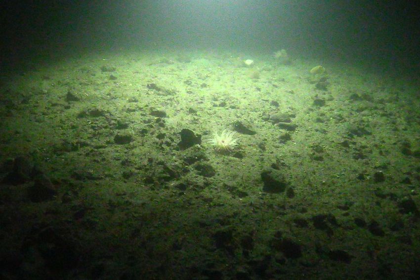
2       Y. Song et al.

decades. With the rapid development of underwater robotic techniques, UUVs
are able to autonomously reach and to measure even in several kilometer wa-
ter depth nowadays, providing platforms for carrying various sensors to explore,
measure and map the oceans.
    Optical sensors, e.g. cameras, are able to record the seafloor as high resolution
images which are advantageous for human interpretation. Consequently, many
UUV platforms are equipped with camera systems for visual mapping of the
seafloor due to the significant improvement of imaging capabilities during the
last decades. However, underwater computer vision remains less investigated
than on land because underwater images are suffering from several effects, such
as attenuation and scattering, which significantly decrease the visibility and the
image quality. In addition, since no natural light penetrates the deep ocean,
artificial light sources are also needed. This non-homogeneous illumination on
limited-size platforms causes anisotropic backscatter that can not be modeled by
atmospheric fog models, as often done for shallow water in sunlight, and further
degrades image quality. The above effects often make computer vision solutions
struggle or fail in (deep) ocean applications.
    The recent trend to employ machine learning methods for various vision tasks
even increases the performance gap between underwater vision and approaches
on land, since learning methods usually require a large amount of training data
to achieve good performance. However, the lack of appropriate underwater (es-
pecially deep sea) images with ground truth data is a bottleneck for developing
learning-based approaches in this field. Simulation of deep sea images, in par-
ticular with illumination, attenuation and scattering effects could be one way to
obtain development or training material for UUV perception.
    This paper therefore proposes a physical model-based deep sea underwater
image simulator which uses in-air texture images and corresponding depth maps
as inputs to simulate synthetic underwater images with both radiometric and
geometric effects. The simulator considers spotlights (with main direction and
angular fall-off) and with arbitrary poses in the model for the special conditions
in the deep sea. Several optimization strategies are introduced to improve the
computational performance of the simulator, which enables us to integrate the
deep sea camera simulation into the common underwater robotic simulation
platforms (e.g. the Gazebo based UUV simulator [10]).

2   Related Work and Main Contributions

Light rays are attenuated and scattered while traversing underwater volumes,
which can be formulated by corresponding radiometric physical models [14].
[7] and [13] decompose underwater image formation into three components: di-
rect signal, forward-scattering and backscatter, which is known as the Jaffe-
McGlamery model. [17] describes the underwater image formation for shallow
water cases. Underwater image formation has been intensively studied in under-
water image restoration that can be considered as the inverse problem of under-
water image formation. The most widely applied model has been presented by
Deep Sea Robotic Imaging Simulator 3
[6], which was initially used to recover the depth cues from atmospheric scatter-
ing images (e.g. in fog or haze in sunlight):
I = J · e−η·d + B · (1 − e−η·d ). (1)
In the above fog model, the image I is described as a weighted linear combination
of object color J and background color B. Here, d is the distance between the
camera and scene point, while η represents the attenuation coefficient.
Current underwater image simulators are mostly based on the fog model: [22]
adds a color transmission map and presents a method to generate synthesized
underwater images, given an ”in-air” image and a depth map that encodes, for
each pixel, the distance to the imaged 3D surface. In the literature, such pairs of
color images (RGB) and depth maps (D) are also called RGB-D images, and we
will use this notation also for the remainder of this paper. [11] proposes a gen-
erative adversarial network (GAN) - WaterGAN, which has been trained with
shallow water images. It also requires in-air RGB-D images as the input to gener-
ate synthetic underwater images. The target function of the GAN discriminator
is also based on the fog model.
However, the fog model is only valid in shallow water cases, where the scene
has global homogeneous illumination from the sunlight. [1] addresses many weak-
nesses of this model, which introduces significant errors in both direct signal and
backscatter components.
Obviously, the fog model does not apply to deep sea scenarios where arti-
ficial light sources are required to illuminate the scene and the resultant light
distribution is extremely inhomogeneous. The light originates from the artifi-
cial sources attached to the robot and interacts with the water body in front of
the camera, leading to very different visual effects in the images, especially in
the backscatter component (see Fig. 1). Hence, the underwater image formation
model in deep sea requires additional knowledge about the light sources like
corresponding poses and properties. [21] uses the recursive rendering equation
adapted onto underwater imagery considering point light sources in their model.
[18] proposes an underwater renderer based on physical models for refraction,
but not focusing on realistic light sources. Since backscatter is computed for
each pixel for each image, the simulation is quite demanding and does not allow
real-time performance. For image restoration rather than simulation, [5] consid-
ers a spotlight with Gaussian characteristics in the image formation model and
applies it to restore the true color of underwater scenes. Consequently, there is
no simulator available to the community that generates realistic deep sea image
sequences at interactive frame rates.
A key use case for deep sea image simulation is integrating it into a UUV
simulation platform, which enables developing, testing and coordinating per-
formance of underwater robotic systems before risking expensive hardware in
real applications. Current ray-tracing solutions are too heavy to integrate to
real-time robotic simulation platforms. For instance, general robotic simulators
provide the simulation of normal camera and depth sensor, which could be ex-
tended to undewater cases. [16] developed a software tool called UWSim, for4 Y. Song et al.
Fig. 1. Different artificial lighting configurations strongly affect the appearance of deep
sea images, especially the backscatter pattern (light cones), which can not be modeled
by the fog model.
visualization and simulation of underwater robotic missions. This simulator in-
cludes a camera system to render the images as seen by underwater vehicles
but without any water effect. [12] extended the open-source robotics simulator
Gazebo to underwater scenarios, called UUV Simulator. This simulator uses so-
called RGB-D sensor plugins to generate the depth and color images, and then
converts them to underwater scenes by using the fog model (Eq. 1).
Another RGB-D based underwater renderer [4] applies trained convolutional
neural networks to style transfer the image output from [12] and additionally add
forward scattering and haze effect. However, their improvements still rely on the
fog model and the haze addition just manually adds two bright spots, which lacks
physical interpretations. [3] integrated the ocean-atmosphere radiative transfer
(OSOA) model into their simulator SOFI and created look-up tables to compose
the back scatter component. However, the OSOA model only describes the sun-
light transformation at the ocean-atmosphere interface, which is only suitable
for shallow water scenarios.
The main contributions of this paper are: (1) A deep sea underwater im-
age solution based on the Jaffe-McGlamery model considering multiple spot-
lights (with angular characteristics) with corresponding poses and properties.
(2) Analysis of the components in the deep sea image formation model and sev-
eral optimizations to improve the simulator’s performance in particular for rigid
robotic configurations. (3) Integration of the deep sea imaging simulator into
the UUV robotic simulator, which can be applied for underwater robotic de-
velopment and rapid prototyping. (4) Open source renderer for facilitating the
development and testing in underwater vision and robotics communities.
3 Deep Sea Image Formation Model
In the deep sea scenario, there is no sun light to illuminate the scene. Only
artificial light sources, which are attached to the underwater vehicles, provide
the illumination. This moving light source configuration makes the appearance
of deep sea images strongly depend on the geometric relationships between the
camera, light source and the object (see Fig. 2).Deep Sea Robotic Imaging Simulator 5
Z
Light source
Camera
d!’ ψ d ’ θ’
φ
Optical axis θ Central axis
Voxel in
water body
d!
d
Y
Surface normal
α
Object
X
Fig. 2. Geometry components involved in the deep sea image formation model (modi-
fied from [18]).
3.1 Radiation of Light Source
This paper considers spotlights, which are commonly used on the UUV plat-
forms. This type of light source usually has the highest light emanation along its
central axis and an intensity drop-off with increasing angle to the central axis.
This angular characteristic can be formulated as radiation intensity distribution
(RID) curve. Often the RID is approximated using a Gaussian function (see e.g.
[5]).
In our simulator it is also possible to directly use the interpolated measure-
ments using a lookup-table and interpolation (see Fig. 3 for a near-Gaussian
curve). In the Gaussian model, the radiance along each light ray can be calcu-
lated as:
1 θ2
Iθ (λ) = I0 (λ)e− 2 σ2 . (2)
Where Iθ (λ), I0 (λ) are the relative light irradiance at angle θ and the maximum
light irradiance along the central axis respectively. The dependency on the wave-
length λ can be obtained from the color spectrum curve of the LED, which is
often provided by the manufacturer or can be measured by a spectrophotometer.
3.2 Attenuation and Reflection
Light is attenuated when it travels through the water, where the loss of irra-
diance depends on the traveling distance and the water properties. Different
wavelengths of light are absorbed with different strengths, which causes the
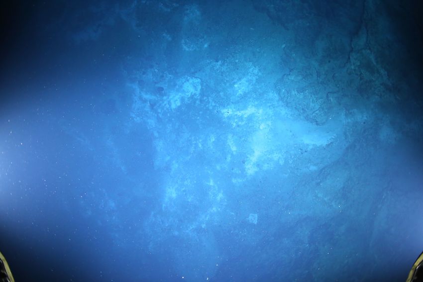
radiometric changes in underwater images. This is because different types of wa-
ter hold different water attenuation coefficients, resulting in variations of color
shifts in images (e.g. coastal water images often appear more greenish, while the
deep water images appear more blueish, see Fig. 4). [8] measured and classified
Earth’s waters into five typical oceanic spectra and nine typical coastal spectra.
[2] shows how the corresponding attenuation curves vary between the different6 Y. Song et al.
1
0.8
Radiant Intensity
0.6
0.4
0.2
0
-80 -60 -40 -20 0 20 40 60 80
Angle to the Centerline [°]
Fig. 3. Radiation characteristics of the light source used in this paper, blue dots: our
underwater lab measurement, red line: its approximation by using a scaled Gaussian
function (σ = 35◦ ).
types and can serve as a first approximation for typical coefficients (and their
expected variations). Due to the point source property of the spotlight , the
Inverse Square Law must be applied in order to simulate the quadratic decay of
the light irradiance along the distance from the point-source it originated from.
When we combine the attenuation effect with the object reflection model, which
assumes light is reflected equally in all directions on the object surface (Lam-
bertian surface), the entire attenuation and reflection model can be formulated
as:
e−η(λ)(d1 +d2 )
E(λ) = J(λ) · Iθ (λ) cos α. (3)
d21
Here, E(λ) is the irradiance which arrives at the pixel of the image and J(λ) is
the object color. The attenuation parameter η indicates the strength of irradi-
ance attenuation through the specific type of water on wavelength λ. d1 and d2
refer to the distance from light to object and from object to camera, respectively.
α indicates the incident angle between the light ray from the light source and
surface normal. In the multiple light sources case, the computation is a summa-
tion of camera viewing rays for all light sources. Note that the denominator only
contains d1 because with increasing d2 each pixel will simply integrate the light
from a larger surface area.
Fig. 4. Different types of water appear in different colors. Left: coastal water in Baltic
Sea. Right: deep sea water in SE Pacific.Deep Sea Robotic Imaging Simulator 7
3.3 Scattering
The rendering of scattering in this paper is based on the Jaffe-McGlamery model,
and is the most complex part of the involved physical models due to its accu-
mulative character. In the Jaffe-McGlamery model, the scattering is partitioned
into two parts: forward scattering and backscatter. Forward scattering usually
describes the light which is scattered by a very small angle, resulting in unsharp-
ness of the scene in the images. This paper approximates the forward scattering
effect with a Gaussian filter g(d) and the size of filter mask depends on the local
scene depth d. We neglect the forward scattering from light to the scene because
the RID curve of the light is usually very smooth (e.g. modeled as a Gaussian
function), where a small extra smoothing can be neglected. Backscatter refers
to light rays which are interacting with ocean water and scattered backwards
to the camera, this leads to a ”veiling light” effect in the medium. This effect
is happening along the whole light path. Following [13], the 3D field in front of
the camera can be discretized by slicing it into several slabs with certain thick-
nesses, the irradiance on each slab is then accumulated in order to form up the
backscatter component:
0 0
e−η(λ)(d1 +d2 )
0 0
E (λ) = Iθ (λ)
d02
1
Ef0 (λ) = E 0 (λ) ∗ g(d02 ) (4)
PN
Eb (λ) = i=1 β(π − ψ)[E 0 (λ) + Ef0 (λ)]∆zi cos(ϕ).
Eq. 4 gives the computation of the backscatter component from each light source.
Here i indicates the slab index and E 0 (λ) denotes the direct irradiance reaching
slab i. d01 and d02 represent the distances from slab voxel to light source and
camera respectively. Ef0 (λ) denotes the forward scattering component of the
slab which convolves E 0 (λ) by the Gaussian filter g(d02 ) and ∗ indicates the
convolution operator. β(π − ψ) refers to the Volume Scattering Function (VSF),
where ψ is the angle between the light ray that hits the voxel and the light ray
scattered from the voxel to the camera (see Fig. 2). The VSF model in this paper
applies the measurements from [15] but can be adapted easily to other VSFs.
∆zi is the thickness of the slab and ϕ is the angle between the camera viewing
ray and the central axis.
[7,18,5] also consider optics and electronics of the camera (e.g. vignetting, lens
transmittance and sensor response) in their models. They are needed to simulate
the image of a particular camera and could be added also to our simulator if
needed. This is however out of scope for this contribution, where we focus rather
on efficient rendering of realistic backscatter. As discussed in [19], underwater
dome ports can be adjusted in a way to avoid refraction, which is why we also
consider adding refraction as a non-mandatory step for underwater simulators
(if needed it can be added using the methods proposed in [18,20]).8 Y. Song et al.
Original Image Depth Map Lighting Setup
1
2 Backscatter
Lookup Table
Direct Signal
4
3
Backscatter
Forward Scattering
5
Underwater Color Image
6
Resulting Image
Fig. 5. Workflow.
4 Implementation
This section shows the implementation of our deep sea robotic imaging simulator.
The complete workflow is illustrated in Fig. 5.
1. Establish the 3D backscatter lookup table, each unit cell accumulates the
backscatter elements along the viewing ray from the camera which is calcu-
lated by Eq. 4.
2. Compute the forward scattering component by smoothing the direct signal
through a Gaussian filter.
3. Generate the direct signal component considering attenuation and object
surface reflection according to Eq. 4.
4. Interpolate the backscatter component from the backscatter lookup table
with respect to the depth value from the depth map.
5. Form up the underwater color image by combining the direct signal, forward
scattering and the backscatter component.
6. Optionally, add refraction effect to the image.
Several optimization procedures are employed in order to improve the perfor-
mance of the deep sea imaging simulator, as described in the following.
4.1 Optimizations for Rendering
In deep sea image simulation, one of the most computationally costly parts
is the simulation of the backscatter component. Backscatter happens through
the water body between the camera and the 3D scene, which is an accumulative
phenomenon in the image. However, when the relative geometry between camera
and light source is fixed, given the same water, backscatter remains constant in
the 3D volume in front of the camera. For example, if there are no objects but
only water in front of the camera, the image will be relatively constant and only
contains the backscatter component. Once the object appears in the scene, theDeep Sea Robotic Imaging Simulator 9
backscatter volume is cut depending on the depth between the object and the
camera, the remaining part is accumulated to form up the image backscatter
component.
...
.
.. {
Δz#
Slab 4
Slab 3
Δz"
{
Slab 2
Δz$
{
Slab 1 Δz% {
Camera Light
Fig. 6. Pre-rendered backscatter field, each unit cell in the slab (green) stores the
accumulated backscatter component (yellow) along the camera viewing ray.
To this end, we construct a 3D frustum of a pyramid for the camera’s field of
view and slice it into several volumetric slabs with certain thicknesses parallel to
the image plane (see Fig. 6). Each slab is rasterized into unit cells according to the
image size. We pre-compute the accumulative backscatter elements for each unit
cell and store them in a 3D lookup table. Since the backscatter component of each
pixel is an integration of all the illuminated slabs multiplied by the corresponding
slab thickness along the viewing ray, the calculation of the backscatter for a pixel
with depth D then is simplified by interpolating the value between the closest
two unit cells along the viewing ray.
During the rendering of the slabs, we noticed that in practically relevant UUV
camera-light configurations, the backscatter component appearance is dominated
by the irradiance from the water volume close to the camera and scattering be-
comes smoother and eventually disappears in the far field. This depends strongly
on the relative pose of the light source(s) and is different in each individual cam-
era system but this is a fundamental difference to the shallow water cases, where
also far away from the camera a lot of light from the sun is still available. Sample
”scatter irradiance” patterns on slabs can be seen in Fig. 9. In order to generate
an accurate backscatter component with less number of slabs, we propose an
adaptive slab thickness sampling function based on Taylor series expansion of
the exponential function:
N (i−1)
∆zi = s · (i = 1, 2, ..., N ) (5)
(i − 1)!
where ∆zi indicates the slab thickness of slab index i. The scale factor s =
2.2 · dmax /eN , where dmax refers to the maximum depth of the scene field which10 Y. Song et al.
is divided into number of slabs N . Here, eN normalizes the Taylor series and
2.2 · dmax ensures the slab thickness is monotonically increasing in (1 < i < N )
PN
and i=1 ∆zi ≈ dmax , (N > 3). This equation leads to denser slab samplings
closer to the camera. As it is shown in Fig. 7, under the light setup described
in its caption, the brightest spot should be at the bottom right corner of the
image. The sampling of slab thickness by Eq. 5 gives a more plausible backscatter
rendering result than the equal distance sampling approach.
Fig. 7. Rendering of backscatter component under the same setups (dmax = 10m,
N = 3, single light which is at (1m, 1m, 0m) in camera coordinate system and pointing
parallel to the camera optical axis.) with different slab thickness sampling approaches.
Left: by equal distance sampling, Right: by Eq. 5.
1
0.9
0.8
Relative backscatter irradiance
0.7
0.6
0.5
0.4
0.3
0.2
0.1
0
0 1 2 3 4 5 6 7 8 9 10
Distance to the camera [m]
Fig. 8. Normalized backscattered irradiance along camera optical axis at different
depth of slabs. Each curve describes the backscatter behavior of Jerlov water type
II with the same light settings as Fig. 7. It can be seen that in this configuration al-
most no scattered light reaches the sensor from more than 8m distance. This puts an
upper limit on the extent of the lookup table for backscatter.
The value of maximum depth of the scene dmax is also an important factor
which affects the backscatter rendering quality and performance. In Fig. 8 we
demonstrate the normalized backscattered irradiance of the voxels along the
optical center axis in deep ocean water. This figure can be a good reference forDeep Sea Robotic Imaging Simulator 11 Fig. 9. Backscatter components of different slabs from 0.5m to 7.5m depth (Second row images’ intensities are amplified 10 times). finding dmax to simulate the underwater images under different conditions or settings. 4.2 Rendering Results As it is shown in Fig. 10, (a) and (b) are the inputs from the RGB-D sensor plugin. The direct signal (c) and backscatter (d) components are computed re- spectively, then the simulated underwater color image (e) is constructed by the direct signal, the smoothed direct signal (forward scattering) and the backscat- ter. In the end, the refraction effect is added to the underwater color image in (f) by using the method from [20]. 4.3 Integration in Robotic UUV Simulation Platform Gazebo is an open-source robotics simulator. It utilizes one out of four different physics engines to simulate the mechanisms and dynamics of robots. Addition- ally, it provides the platform for hosting various sensor plugins. [12] proposes the UUV Simulator which is based on Gazebo and extends Gazebo to underwater scenarios. The UUV Simulator additionally takes into account the hydrodynamic and hydrostatic forces and moments for simulating vehicle dynamics in underwa- ter environments. Several sensor plugins which are commonly deployed on UUVs are also available, including: inertial measurement unit (IMU), magnetometer, sonar, multi-beam echo sounders and camera modules. We integrate our deep sea camera simulator into the UUV Simulator camera plugin which provides in-air and depth images as the input and it is able to reach interactive speeds for 800×800 size of images using OpenMP without any GPU acceleration on a 16-core CPU (Intel Xeon W-2145 CPU @3.70GHz) consumer hardware. The workspace interface and sample rendering results are shown in Fig. 11.
12     Y. Song et al.

      (a) in-air           (b) depth        (c) direct signal      (d) backscatter

               (e) underwater color                (f) add refraction

                     Fig. 10. Deep sea image simulation results.

5    Evaluation

We evaluate our deep sea image simulator by comparing with three state-of-
the-art methods, which use in-air and depth images as the input to synthesize
underwater images: UUV Simulator [12], WaterGAN [11] and UW IMG SIM
[4]. Due to the image size limitation from WaterGAN, all the evaluated images
are simulated in the size of 640×480, although our method does not have this
limitation.
    To render the realistic deep sea images close to the images shown in Fig.
1, we initialize the camera-light setups as: two artificial spotlights which are
1m away from the camera on the left and right sides, both tilt 45◦ towards
to the image center. The real image was taken in the Niua region (Tonga) in
south pacific ocean, according to the map of global distribution of Jerlov water
types from [9], water in this region belongs to type IB and the corresponding
attenuation parameters are (0.37, 0.044, 0.035)[m−1 ] for RGB channels. The
simulation comparisons are given in Fig. 12. We create an in-air virtual scene
with a sand texture, and simulate the corresponding underwater images by using
the different methods. Since only our method considers the impact of lighting
geometry configuration, the other methods are not able to add the shading effect
on the texture image. To fairly compare our approach to others, we first add
the in-air shading in the texture image and feed it to the other simulators,
even though this in-air shading with a specific light RID is not available in any
standard renderers.
Deep Sea Robotic Imaging Simulator 13
Fig. 11. Left: camera path overview in simulator. Right: Rendered image sequence.
Due to the physically correct model, already in the simulation we can see that some
images will be overexposed with the settings chosen. Consequently, the exposure control
algorithm of the robot can be adapted already after simulation without wasting precious
mission time at sea.
As it is shown in Fig. 12, the UUV Simulator is only able to render the
attenuation effect based on the fog model without considering the impact of the
light sources, the backscatter pattern caused by lighting is completely missing
in their image. Their attenuation effect only considers the path from the scene
points to the camera, which makes the rendered color also not conform to the
deep sea scenario. The same problem also occurs in the WaterGAN results,
due to the lack of deep sea images with depth maps and ground truth in-air
images, the GAN is trained using the parameters given in the official repository1
on the Port Royal, Jamaica underwater dataset2 . Therefore the color and the
backscatter pattern of the light source is highly correlated with the training data
which does not fulfill the setup in this evaluation case. UW IMG SIM presents
the backscatter pattern of the light source. However this effect is just adding
the bright spots into the image without any physical interpretation, their direct
signal component also has no dependence to the light source, which also is not
realistic. Our proposed approach captures all discussed effects present in real
images better than the other methods, it not only renders the color much closer
to the real image, but also simulates attenuated shading on the topography
and back scatter caused by the artificial light sources which is missing in other
approaches.
6 Conclusion
This paper presents a deep sea image simulation framework readily usable in
current robotic simulation frameworks. It considers the effects caused by arti-
ficial spotlights, and provides good rendering results in deep sea scenarios at
interactive framerates. Earlier underwater imaging simulation solutions are ei-
ther not physically accurate, or far from real-time to be integrated into a robotic
1
https://github.com/kskin/WaterGAN
2
https://github.com/kskin/data14 Y. Song et al.
(a) in-air (b) depth (c) our output
(d) in-air shading (e) UUV (f) WaterGAN (g) UW IMG SIM
Fig. 12. Outputs of different underwater image simulators for the same scene.
simulation platform. By detailed analysis of the deep sea image formation com-
ponents, based on the Jaffe-McGlamery model, we propose several optimization
strategies which enable us to achieve interactive performance and makes our
deep sea imaging simulator fit to be integrated into the robotic UUV simulator
for prototyping or task planning. We also apply this renderer for AUV lighting
optimization in our later work. We will release the source code of the deep sea
image converter to the public to facilitate generation of training datasets and
evaluating underwater computer vision algorithms.
References
1. Akkaynak, D., Treibitz, T.: A revised underwater image formation model. In: Pro-
ceedings of the IEEE Conference on Computer Vision and Pattern Recognition.
pp. 6723–6732 (2018)
2. Akkaynak, D., Treibitz, T., Shlesinger, T., Loya, Y., Tamir, R., Iluz, D.: What is
the space of attenuation coefficients in underwater computer vision? In: 2017 IEEE
Conference on Computer Vision and Pattern Recognition (CVPR). pp. 568–577.
IEEE (2017)
3. Allais, A., Bouhier, M., Edmond, T., Boffety, M., Galland, F., Maciol, N., Nicolas,
S., Chami, M., Ebert, K.: Sofi: A 3d simulator for the generation of underwater
optical images. In: OCEANS 2011 IEEE - Spain. pp. 1–6 (2011)
4. Álvarez-Tuñón, O., Jardón, A., Balaguer, C.: Generation and processing of sim-
ulated underwater images for infrastructure visual inspection with uuvs. Sensors
19(24), 5497 (2019)
5. Bryson, M., Johnson-Roberson, M., Pizarro, O., Williams, S.B.: True color correc-
tion of autonomous underwater vehicle imagery. Journal of Field Robotics 33(6),
853–874 (2016)Deep Sea Robotic Imaging Simulator 15
6. Cozman, F., Krotkov, E.: Depth from scattering. In: Proceedings of IEEE Com-
puter Society Conference on Computer Vision and Pattern Recognition. pp. 801–
806. IEEE (1997)
7. Jaffe, J.S.: Computer modeling and the design of optimal underwater imaging
systems. IEEE Journal of Oceanic Engineering 15(2), 101–111 (1990)
8. Jerlov, N.: Irradiance optical classification. Optical Oceanography pp. 118–120
(1968)
9. Johnson, L.J.: The underwater optical channel. Dept. Eng., Univ. Warwick, Coven-
try, UK, Tech. Rep (2012)
10. Koenig, N., Howard, A.: Design and use paradigms for gazebo, an open-source
multi-robot simulator. In: 2004 IEEE/RSJ International Conference on Intelligent
Robots and Systems (IROS)(IEEE Cat. No. 04CH37566). vol. 3, pp. 2149–2154.
IEEE (2004)
11. Li, J., Skinner, K.A., Eustice, R.M., Johnson-Roberson, M.: Watergan: Unsuper-
vised generative network to enable real-time color correction of monocular under-
water images. IEEE Robotics and Automation letters 3(1), 387–394 (2017)
12. Manhães, M.M.M., Scherer, S.A., Voss, M., Douat, L.R., Rauschenbach, T.:
UUV simulator: A gazebo-based package for underwater intervention and
multi-robot simulation. In: OCEANS 2016 MTS/IEEE Monterey. IEEE (sep
2016). https://doi.org/10.1109/oceans.2016.7761080, https://doi.org/10.1109%
2Foceans.2016.7761080
13. McGlamery, B.: A computer model for underwater camera systems. In: Ocean
Optics VI. vol. 208, pp. 221–231. International Society for Optics and Photonics
(1980)
14. Mobley, C.D.: Light and water: radiative transfer in natural waters. Academic press
(1994)
15. Petzold, T.J.: Volume scattering functions for selected ocean waters. Tech. rep.,
Scripps Institution of Oceanography La Jolla Ca Visibility Lab (1972)
16. Prats, M., Perez, J., Fernández, J.J., Sanz, P.J.: An open source tool for simu-
lation and supervision of underwater intervention missions. In: 2012 IEEE/RSJ
international conference on Intelligent Robots and Systems. pp. 2577–2582. IEEE
(2012)
17. Schechner, Y.Y., Karpel, N.: Clear underwater vision. In: Proceedings of the 2004
IEEE Computer Society Conference on Computer Vision and Pattern Recognition,
2004. CVPR 2004. vol. 1, pp. I–I. IEEE (2004)
18. Sedlazeck, A., Koch, R.: Simulating deep sea underwater images using physical
models for light attenuation, scattering, and refraction (2011)
19. She, M., Song, Y., Mohrmann, J., Köser, K.: Adjustment and calibration of dome
port camera systems for underwater vision. In: German Conference on Pattern
Recognition. pp. 79–92. Springer (2019)
20. Song, Y., Köser, K., Kwasnitschka, T., Koch, R.: Iterative refinement for underwa-
ter 3d reconstruction: Application to disposed underwater munitions in the baltic
sea. ISPRS - International Archives of the Photogrammetry, Remote Sensing and
Spatial Information Sciences XLII-2/W10, 181–187 (2019)
21. Stephan, T., Beyerer, J.: Computergraphical model for underwater image simula-
tion and restoration. In: 2014 ICPR Workshop on Computer Vision for Analysis
of Underwater Imagery. pp. 73–79. IEEE (2014)
22. Ueda, T., Yamada, K., Tanaka, Y.: Underwater image synthesis from rgb-d images
and its application to deep underwater image restoration. In: 2019 IEEE Interna-
tional Conference on Image Processing (ICIP). pp. 2115–2119. IEEE (2019)You can also read