The Comprehensive Optimal Business Location Model
←
→
Page content transcription
If your browser does not render page correctly, please read the page content below
The Comprehensive Optimal Business Location Model

                                                                                                                                                                                                                                    Mitchel Gorecki1
                                                                                                                                                                                                                         Professor Charles Becker, Faculty Advisor

                                                                                                                                                                                                                                      Duke University
                                                                                                                                                                                                                                   Durham, North Carolina
                                                                                                                                                                                                                                           2011


1 Mitchel Gorecki is currently completing a Bachelor of Science in Biomedical Engineering, a Bachelor of Science in
Mechanical Engineering, and a Bachelor of Science in Economics with a concentration in Finance. The author can be
reached at mitchel.gorecki@duke.edu. He would like to thank Professor Charles Becker for his great mentorship in the
completion of this project.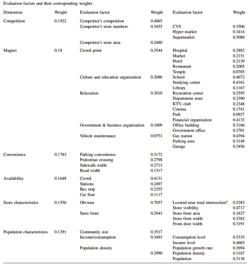
                                                                                                 1


                                             Abstract

       In order to ensure long run viability, a firm must understand the idea of optimal business
location. In the designing of a strategy, it is important to not only evaluate the present market
environment but to also account for possible future change. This paper will demonstrate the
core ideas behind a comprehensive location model that will predict the optimal location for a
business. The effectiveness of the model will be evaluated by using past data from Durham,
North Carolina to predict current retail development. The model is determined to be successful
by seeing if the trend recognized would be able to correctly identify the present location choices
of firms. The model will be further used to predict the future development plans for businesses
locating in the Durham area.
2
The Comprehensive Optimal Business Location Model
Introduction
The essential idea of the store location model is to identify and weight the key
characteristics of an area that contribute to a business’ success and combine them into a formula
that will indicate the optimal place of establishment. The first step in the process is to identify
what parameters determine a firm’s success. Chi, Kao and Kuo (2010) provide an excellent
breakdown of what aspects mattered most to business location in Figure 1. The parameters
identified were found by comparing a successful business to the factors of the location that
helped contribute to that success. A survey of 138 CVS stores in Taiwan was taken, where
variables like profits and patrons per day were used to identify success. These identical firms
were then compared and evaluated based on the characteristics of their location. Certain
characteristics of the locations were shown to contribute differently to success. These entities
were categorized by their type and relativistic impact on a business. The major groups identified
were competition, convenience, availability, store characteristics, and population characteristics.
Within each of these groups are subgroups that provide an even more precise analysis of a
possible location. For instance, convenience is broken down into parking convenience,
pedestrian crossing, sidewalk width and road width. The next step in the model requires that
each parameter be evaluated for its weighted impact on the location. This calls for assigning
each identified parameter a percentage value of importance with regard to the other variables.
The exact weighting is determined by comparing the past successes and failures other firms
given conditions to evaluate the extent to which each parameter impacted the fate of the firm.
So for instance, if 100% of stores sampled were determined to be on average successful, yet
50% of them were near a library, it can be determined that proximity to a library does not
significantly contribute to the success of a firm and should hence have a low contribution to the
success rate formula. So long as the sample of firms is large and representative of all the
variables accounted for, an accurate estimate of the relative success contribution is possible.
These values can be found next to the corresponding category in Figure 1. The next step in the
process is collecting quantifiable data that can be integrated into a final equation. 3
Data Collection
Data are collected via two methods: sampling and surveying. The first method relies on
observing patterns of already established firms and recording data. Figure 2 provided by Chi,
Kao and Kuo (2010) shows a list of the top observations recorded and the method by which the
area is evaluated. However, in many cases it is excessive and time consuming to evaluate an area
in its entirety, so sampling is used. This method relies on the idea of the law of large numbers
and central limit theorem. Rather than obtaining an entire data set, statistical principles allow for
values to be estimated with adequate precision given a smaller sample of that data set. This saves
the firm the cost of money and time when choosing the optimal location for its business. The
components encapsulated in the sample range from measuring road distances between stoplights
to the presence of other businesses like a gas station and even the width of the sidewalk. All of
these observations are evaluated and converted into a score ranging from 0 to 10. This allows
the firm to quantitatively analyze the data. For instance, storefront visibility is a huge factor in a
business’ success. As such, specific road configurations as well as traffic volumes are categorized
into quantitatively measurable scores. A chart showing the values for common configurations
and traffic flow can be found in Figure 3. By identifying which locations are optimal with
respect to roads and traffic, the firm can quantitatively analyze the probability of success from
locating at that specific point. By repeating this process with the other parameters, the firm will
have a way of mathematically determining the optimal location. Rather than incurring the cost of
taking new data, Google Maps, Bing Maps, GIS software were used in this analysis. The majority
of the physical measurements were taken by using tools provided by Google and GIS software
in combination with an array of maps over various periods of time. Although this is a
comprehensive analysis of the surrounding characteristics of a location, it does not evaluate the
attitudes of the consumer.
The second aspect of collecting data is to take surveys of individuals who would become
the primary customers if indeed the firm would locate in a particular location. This is essential
because location alone is not able to perfectly predict the success of a firm. The idea behind a
survey is to gauge the characteristics of the populous that would impact their consumerism. This 4
model uses data from the survey of 138 CVS stores in by Chi, Kao, and Kuo. We can assume
that the people of Durham exhibit consumeristic traits similar to those of the average person.
For that reason, surveys previously taken in these other cities, like Taiwan, can be applied to
Durham. Much like the parameters above, characteristics like population density and income
levels are assigned weighted values. Although the survey takes data across large areas where this
particular model will be focusing on a single selected area. This means the model must consider
a customer’s distance threshold when commuting to the business apart from the other variables.
For this particular variable, the survey showed that the maximum distance the consumer is
willing to travel was negatively proportional to the square of the distance. This is a very
important principle, especially in context of competition, where a similar service can often be
found at a closer location to the consumer. Much like the data taken by sampling, the remainder
of the survey data is converted into quantitative values that can be mathematically manipulated
to create a model.
The Model
With all of the information collected, a model can be made. Rather than attempting to
create a single function in terms of numerous variables, this paper takes the approach of using
meshplots, or three dimensional surface plots. This is done by assigning coordinates in a matrix
to longitude and latitude values that create a grid covering a targeted area. In our case the
selected region is the Brightleaf Square area in Durham, North Carolina. This location was
chosen because of the large amounts of maps and data available as well as the significant amount
of development that has occurred in the last 50 years. Each of the parameters and values above
is different for each point in this grid of locations. Much like the matrix of locations, a matrix is
constructed for each value that is superimposed onto the original matrix map. Some of these
layers will simply be observations taken from the sample, which then get converted into
numerical values. Other layers, like that for commuting distance, will call for calculations of
values given distances from every possible point of location. All of these layers will be properly
weighted and added together, incorporating all of their individual contributions to create a single
surface plot. As these layers of variables are added to the map, some areas of longitudes and 5
latitudes will begin to produce peaks and troughs. The peaks will represent the coordinates on a
map where businesses are most likely to succeed and the troughs where they are least likely.
Once this process is completed, the maximum values of each peak should identify the optimal
location for a given firm. An example of such a matrix would be
0 1 0
!! = 3 6 2 ∗ .1648
4 8 5
where M1 represents a matrix of data that might rank parking availability. Nine points in the
chosen area are evaluated, with each number representing a location on a map as well as the data
taken at that location. In this case the cell (3,2) has the maximum parking availability, with a
value of 8 out of 10. The entire matrix is multiplied by a scaling factor that alters the value to
match their proportional importance. These are the factors described above that are calculated
by comparing the success rates of various businesses with specific parameters to see if there is
any correlation. For parking, each additional point on the 0 to 10 scale contributed a
relative .1648 points when compared to other parameters. The cell (3,2) then translates on a map
the coordinates (longitude, latitude) of the optimal location. When applied on a greater scale, a
data set of matrices is represented by:
!! , !! , … !!
and the weighted parameters are the set such:
!! , !! , … !!
where final cumulative matrix, Z, used to make a surface plot would be:
!
! = !! !!
!!!
The final absolute optimal business location is determined by taking the maximum of the final
matrix Z. Other, local maxima, may exist, so the use of 3D surface plots allows the user to
represent the solution as a surface that can be directly super imposed onto the area in question.
The actual calculations and data are shown in the Matlab script, which is provided at the end of 6
this paper. Although, this identified location will only apply to a generic business. Additional
factors must be considered when dealing with particular businesses, which are addressed once
the model is fully established.
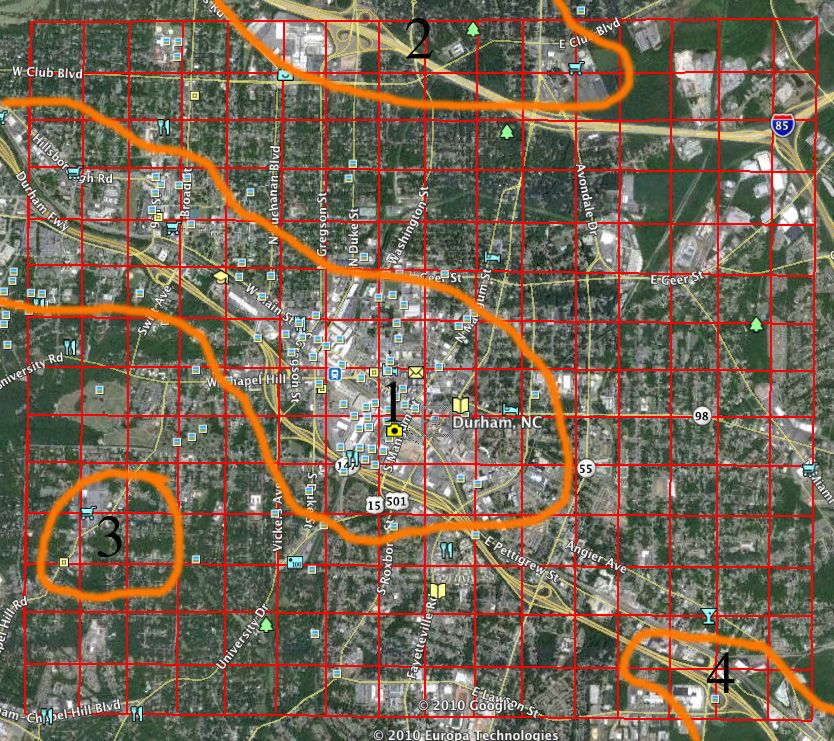
To ensure the functionality of the optimal location finder, the program was run from
data collected off a map of Durham in 1925 (Figure 4) to see which sites back then would have
been considered best. This result can be compared to the actual presence of established
businesses in these sites to determine the level of functionality of the optimal location finder.
The peaks in the meshplot in Figure 6 indicate that that optimal locations for businesses in 1925
were in the areas 1, 2, 3, and 4 as shown in Figure 5. The 2010 map of the same region shows
that the areas identified as high business survival rate areas then are already well populated by a
variety of firms. This indicates that the optimal locations identified from a map from 1925
successfully predicted the same places real firms chose to locate. Assuming these firms made
marginal decisions when choosing a location such that the best spot was chosen, the areas
identified must have indeed been the optimal locations. The key differences between area 1 and
areas 2-4 are the size of the captured area and the cumulative value assigned to that region. The
reason for this discrepancy can be explained by the cost incurred by the consumer when seeking
a firms’ business. This may be partially explainable by the demographic change that occurred
between 1925 and 2010. There was a large movement towards racial integration, particularly in
this area. The average consumer did not drive and as such the cost of business due to location
was much greater. This could possibly indicate why area 1, the point of minimum cost to the
consumer, became the largest center of business growth.
The cost to the consumer increases as the square of the distance traveled to do business.
This means it is in a firm’s best interest to locate at a point where it minimizes the cost to its
consumers, thus increasing the amount of business the firm sees. The optimal point can be
found by graphing the sum of the cost to all considered consumers at every point and finding
the minimum of the graph produced. This is possible even when residential areas have yet to
exist. The model regards undeveloped areas as residential space, although with low population
density. By identifying those areas as residential, the cost to consumer is minimized while
considering future consumer locations. This allows for the model to be applied to a wider range
of situations. Figure 8 shows the graph of consumer cost when considering locations at every 7
point possible. Figure 9 is a color surface of that graph rotated to look straight down on the
graph. The darkest blue areas are those in which the least cost is incurred on part of the
individual to do business with a firm at that point. Notice how the darkest of the blue
concentrates on the region bounded by area 1. This explains for the increased density of firms in
this area compared to others. The combination of these methods allows for the prediction of
both the optimal firm location and major center for commerce for almost 100 years in advance.
Now that the method has been proved accurate in this case, the next step is to use the data and
model to determine the future locations firms will chose.
Application and Analysis
Those places that are optimal for current development can be identified by those areas
on the graph in Figure 4 that produce peaks but are not necessarily maximums. The places of
interest are those locations where development is present but scarce. Such locations are areas 2,
3, and 4. This is because regions like area 1 are already well developed and are limited as to the
number of new opportunities that can be found in the same location. This poses the question as
to how to identify an area that is already experiencing diminishing returns with respect to future
development. The solution is found by comparing those areas that are experiencing diminishing
returns to the meshplot surface and identifying those characteristics that distinguish that area
from another.
The solution is to find peaks where the first partial derivatives with respect to x and y of
the surface found in Figure 6 are between 0 and -1. This means that the slope of the surface at
these points is relatively flat, but still decreasing. Such areas are represented by orange squares
near a peak, rather than sudden transitions from red to blue. Those areas where the first partial
derivatives are greater than 1 or less than -1 tend to quickly transition into residential areas,
halting further business expansion. Mathematically, the same criteria are such that the second
partial derivatives are less than -1. Where this occurs, it can be seen as a limit or boundary where
no new development will readily occur in the future. There is a greater possibility for
development when the area in question transitions from commercial to residential at a slower
rate. This indicates that the area has not reached a level of saturation where business 8
development is hindered. This concept can be graphically represented by using a vector field.
Figure 10 shows a plot of the partial derivatives of the meshplot. The arrows point away from
the peaks, with their lengths correlating to their respective values. The larger arrows indicate a
steeper slope of the surface. Those regions bounded by arrows with values between 1 and -1
mark the future places for business development. In terms of the analyzed area, it is reasonable
to hypothesize that areas 2, 3 and 4 will be key development areas in the next 50-75 years.
Notice how in Figure 6 these places correlate to peaks in the graph where the first partial
derivatives are between 1 and -1 and the second partial derivatives are between 0 and -1. This
theory is testable by comparing these areas identified by the 1925 map to a current map of the
same area.
As expected, those areas that met the correct criteria outlined above experienced the
greatest amount of retain growth. The lots in areas 2, 3, and 4 that were empty in 1925 are
currently filled or under development. As for area 1, Maps of Durham from 1925-2009 show
that the stretch of businesses along Main Street were established much sooner than the other
areas. As such, this sector was already saturated with respect to the number of firms that could
possibly locate in this zone without flooding over into residential areas. Rather than experiencing
new development, it was common to see the same stores change hands or get renovated.
Conclusion for the Generic Firm
All of these principles can be synthesized to create the final model that can predict where
future generic retail locations will develop. Instead of collecting new, more current data, the
same graphs can be used to further hypothesize the future locations of firms. For the reasons
outline above, the places in which development is be expected to occur is in areas 2, 3 and 4. Of
these places, that with greatest opportunity is area 4. This is determined simply by evaluating
which area best fit the previously established criteria.
Using Durham as an example, this comprehensive model has proved its robustness in
determining the location choices of future firms. In the generic situation, the three primary
indicators to a high rate of success for a firm’s given location were determined to be: 9
1. The given area must have a peak when looking at the meshplot of the sum of evaluative
matrixes.
2. Given a highly competitive situation, a firm must understand that primary places of
commerce will form where the cost to the consumer to business is at a minimum.
3. The first partial derivatives in the x and y direction must be between 1 and -1 and the
second partial derivatives between 0 and -1.
These three parameters are the key to ensuring long run viability of a firm. Using Durham,
North Carolina as the example, the model proved to effectively determine the “hotspots” for
businesses. Although, this solution only applies to the generic firm.
Firm-Specific Malleability
The optimal location is vastly different when firm-specific factors are taken into
consideration. No two firms are identical, and will hence give different weights to the most
important factors of the model. For instance, a gas station will chose a location that best reduces
consumer cost even if the area is already over-developed. A restaurant on the other hand will
most likely chose to locate in an area already populated with other businesses, and even other
restaurants alike, just because of the greater consumer exposure. These anomalies make creating
the perfect optimal business location model rather difficult. Although, trends in location choices
of specific types of firms can be used to help fine-tune the model. By altering the weights of the
parameters, the model can be accommodated to suit the needs of a particular firm. Specific types
of firms are grouped by the attributes to which they weight greater than the general firm:
1. Road configuration intensive: This type of firm gets great benefit from exposure to
traffic and storefront view to the road. Common examples are a gas station or fast-food
restaurant. These types of firms are better off locating where there is the greatest
storefront exposure, which is directly related to the road configuration. In this case, the
convenience, availability and store characteristics weights were adjusted to produce the
adjusted graph to the left. Particularly, the weights for these categories were increased to 10
reflect their greater importance. For instance, the
convenience weight was raised from .1783 to .5349,
making the impact of this attribute three times greater
than before. Compared to the generic situation, the
dark red peaks have become much more pronounced.
This is because these areas better suit the firm’s specific
criteria. Note how this area, which almost appears as a
straight line, follows directly along Main Street. What
this indicates is that the optimal location in this situation will be right at beginning of
Main Street as it enters Bright Leaf Square. Interestingly, the firms located in this area are
a gas station, two fast pizza vendors, two clubs and a bar. All of these firms are indicative
of road configuration intensive firms.
2. Consumer exposure intensive: This category of
firm gives greater importance to the
convenience matrix, with the addition of
augmenting the importance of minimizing the
cost to the consumer. Much like the situation
above, the convenience weighting is increased
from .1783 to .8915. An example of such firms
would be a club or restaurant. The adjusted graph can be seen to the right. The first
observation is that the rough peaks surrounding the main, center peak have all been
flattened. Other than the primary stretch along Main Street, no other locations indicate a
greater probability of success. The only peak is in the same location as identified by the
consumer cost minimization surface. This makes sense since as the location moves away
from this center area, the firm would be farther away from its average customer. This is
not optimal, since this type of firm relies on consumer exposure for the bulk of its
business. This is an excellent example showing how it is vital that a firm is able to
recognize which factors are most important to its success. This type of a firm is goes
directly against the general trend. Those areas that were previously identified as places for
future development exhibit no indications of growth for this type of firm. Had the firm 11
been unaware of this concept, it would not be able to correctly identify its optimal
location.
3. Competition proximity intensive: This type of firm actually benefits from the presence of
competing firms due to their joint ability to attract more customers as a whole. The
primary example of such a firm is a restaurant. When grouped together, the area is more
likely to draw customers. This is directly related to the
consuming characteristics of the individual. The model is
adjusted to this type of firm by changing the weighted
parameters for competition and convenience. Both
values were increased by a factor of three. Notice how
for this type of firm, the adjusted graph is heavily
centered on the Brightleaf Square area. The primary type
of businesses in this region are restaurants, just as the model predicted. The surprising
aspect of this success surface is how the competition of other firms actually attributed to
the success of neighboring business. The areas 2, 3 and 4 that were identified as future
places of growth for the generic firm are almost nonexistent. This can be explained by
the lack of presence of other restaurants in these areas. Rather than attempting to success
in isolation, it is best for a new restaurant to locate near other competitors. This can be
interpreted as increasing exposure to consumers who are already looking to purchase a
meal. This way the business is most likely to be closest to the largest group of people
looking to do business with that particular type of firm.
4. Appreciating isolation: This type of firm has minimal criteria for a location and only
makes its chose with the hope that at some point the land will appreciate. Its location
choice is solely based on cost minimization, rather
than focusing on optimizing consumer interaction.
Such a type of firm is a small factory, distribution
center, or even mechanic. These types of
businesses ultimately disregard factors like 12
convenience, store characteristics and availability. Rather, the main decision factor is
competition. As such, the weighting is altered to nearly only account for competition.
This parameter is increased in importance, while the others like convenience, availability
and store front are decreased in weight. Unlike the restaurant example where firms
prosper when congregated, this type of business is best of scattering across more rural
areas. The adjusted success surface depicts just this. The main stretch along Main Street
is nearly worthless to this particular firm. Rather, areas 3 and 4 as well as the entire
eastern edge produce peaks, indicating the greatest probability of success. This is because
these areas have developed roadways, but are scarce with respect to the number of
business. This is nearly the perfect situation for a firm that choses its location primarily
based on competition. These observations cannot be compared to the actual presence of
firms in these areas because they have yet to develop. Although, based on the cleared
areas and construction equipment present today, it is reasonable to assume that such
types of firms will be established in this area in the next ten years or so.
Conclusion
Optimal business location plays a crucial role in the establishment of a firm. A given
business is bound to fail without an understanding of how the characteristics of a particular
location impact a firms’ success. Although there is no perfect solution that can be applied in all
scenarios, there are a myriad of parameters that can be tailored to meet the needs of nearly any
firm. This model allows a business to not only evaluate the present market environment but to
also account for possible future change in an area. The city of Durham, North Carolina
provided the example that demonstrated the power of understanding the optimal location model.
This power extends beyond that of predicting sites for future successful business development,
providing insight to other areas of business.
In economics, it is nearly always true that in the presence of asymmetric information
there is an opportunity to profit. The asymmetry in this situation is that the model provides an
empirical method to evaluating a successful area for business growth. By knowing this before it
occurs, it allows the individual to capitalize through means of investment in land or 13
development of an area. Indeed this can be seen as a risk, since there is no guarantee that a given
area will appreciate. Although, compared to the average investor, the user of this model will
have a significant advantage when choosing the area in which to invest. This helps answer many
questions, such as to where the next big retail area will develop.
Further applications of this model call for collecting data over large-scale areas in an
attempt to predict the future development plans for businesses. For Durham, North Carolina,
this would mean examining areas such as the Fayetteville corridor from highway 147 to
Southpoint shopping center. The key to such an analysis would be to predict where exactly firms
will most likely locate as well as what types of firms will most likely chose this location. The
difficulty in this analysis is that each particular firm will chose its location with differently
weighted parameters. In order to identify what kinds of firms will locate in this area, the model
would have to be applied for every type of firm, similar to the outline above. Another important
area of interest is the stretch from NC Central to NC-54. A model of this area would provide
insight as to whether or not the dream of a continuous stream of commerce is reasonable. That
said, there is one remaining problem.
This model is a passive indicator of relative probabilities of success. It is not an active
predictor that can dictate a firm’s location choices. The model relies on using past data to
determine correlations between variables to then draw a conclusion regarding the statistically
optimal location. By no means does this guarantee that the location identified is the optimal
choice. Rather, it is the optimal location given the choices of other preceding firms. What this
means is that there will always be anomalies that will force the model to adjust. For instance, an
independent McDonald’s establishment will rarely choose to locate in an already developed area.
This is because a primary source of income to many of these fast-food chains is the lease of
surrounding land to other developers, rather than the sale of food. Other firms know that
McDonald’s greatly attracts consumers and will chose to locate near these establishments,
despite having to pay rent to the fast-food chain. This deviates from the major trends identified
in the model. This means it could not accurately predict the location choices of firms like
McDonald’s with as great of confidence as other firms. These anomalies are indicative of many
big-name businesses. Regardless, the model still proves a vital tool for smaller firms, developers
and those wishing to attain an accurate prediction of how future successful businesses will locate. 14
Figures
Figure 1: key parameters and weight values (Chi, Kao and Kuo) 15
Figure 2: aspects considered when sampling an area (Chi, Kao and Kuo) 16
Figure 3: assigning values to specific road configurations and traffic volumes (Chi, Kao and Kuo)
Figure 4: map of Durham from 1925
Provided by Digital Durham 17
Figure 5: a map of Durham in 2009 with key areas identified (Google Maps)
Figure 6: a 3D meshplot of cumulative data Figure 7: the colorized surface of the meshplot
Figure 8: a surface plot of cost to the individual Figure 9: the colorized consumer cost surface 18
Figure 10: a vector field of derivatives of the meshplot surface 19
Matlab Code
%% Urban Economics - Econ245 :: Optimal Business Location Finder
%% By Mitchel Gorecki
clear
clc
% make matrix values
[x y] = meshgrid(1:1:17, 1:1:15);
competition = [10 9 9 9 8 6 6 7 8 9 7 5 6 10 8 8 9;
10 10 9 6 7 6 6 8 8 8 5 4 8 8 6 8 8;
5 6 7 8 9 10 9 9 9 8 7 6 6 7 6 8 9;
4 5 6 6 4 5 7 8 5 5 6 7 8 9 9 5 5;
3 4 5 4 4 6 5 7 4 5 5 3 2 5 2 2 2;
5 4 4 5 5 6 4 5 4 5 5 4 1 2 2 4 2;
8 9 9 8 7 3 1 1 0 1 3 5 8 8 7 8 9;
10 9 8 6 5 3 1 0 0 2 4 4 4 6 8 8 9;
10 10 8 6 6 5 0 0 0 0 2 3 3 4 5 3 2;
10 9 9 9 8 8 8 5 0 1 2 3 4 5 6 7 3;
7 3 4 5 6 8 8 6 2 1 1 2 3 4 5 8 8;
8 7 8 9 6 5 4 2 2 2 2 3 4 4 5 8 7;
8 9 8 9 8 10 5 5 6 6 5 5 5 6 4 7 8;
8 7 8 8 8 9 9 6 4 4 5 6 5 5 5 5 6;
4 3 3 5 7 8 6 4 3 4 5 6 4 4 6 7 5].*.1922;
convenience = [0 1 2 3 4 5 8 8 4 2 3 3 2 1 0 0 2;
1 0 1 1 2 1 1 1 8 7 6 6 2 0 2 2 0;
8 5 4 3 2 1 1 2 1 2 0 0 0 2 2 2 2;
10 8 5 6 4 1 1 1 1 2 2 2 2 0 0 4 8;
8 9 10 8 6 5 6 5 4 3 2 2 7 2 5 6 9;
10 9 8 8 7 6 5 6 6 5 4 3 7 6 6 5 4;
1 1 2 3 10 10 8 6 8 8 7 5 3 2 2 1 1;
1 2 2 3 8 8 10 10 10 8 5 5 4 2 1 3 1;
0 2 3 2 1 5 8 10 10 8 7 5 4 2 2 5 4;
1 3 4 2 2 1 5 8 7 8 6 3 3 2 1 1 4;
2 7 6 3 1 2 3 2 7 7 3 2 1 1 1 1 1;
2 4 0 0 2 3 3 2 1 5 7 6 4 3 1 1 0;
2 1 2 0 0 0 3 4 4 2 2 6 6 8 3 2 1;
1 3 3 2 0 0 2 2 2 3 2 1 2 5 5 5 4;
8 9 8 6 2 0 2 4 4 5 4 3 5 5 4 5 6].*.1783;
availability =[0 1 1 4 5 8 10 10 3 1 1 1 1 0 0 0 2;
2 1 1 2 2 4 5 6 3 2 4 8 2 0 4 5 3;
8 6 4 2 1 1 1 0 0 1 3 2 2 2 4 4 4;
10 9 8 7 6 4 2 1 0 0 2 1 0 0 0 3 8;
10 10 10 10 9 7 5 5 2 1 0 2 5 0 4 6 6;
8 8 9 9 10 8 7 6 8 5 2 1 8 9 2 3 5;
1 2 0 0 9 10 10 10 8 6 2 2 3 2 0 1 2;
1 0 2 2 3 8 10 10 10 8 4 4 3 2 1 1 1; 20
0 0 1 2 3 8 10 10 10 8 5 4 5 3 2 8 5;
2 2 1 1 2 3 8 10 9 9 8 5 4 3 1 1 7;
2 7 6 5 4 1 1 3 5 4 3 2 1 1 1 1 0;
0 3 0 0 0 3 2 2 3 3 5 5 4 2 2 1 0;
2 1 0 0 0 0 2 5 4 4 3 7 8 8 8 3 2;
1 3 2 1 2 0 3 4 5 3 2 1 1 5 5 5 0;
8 7 8 5 3 2 2 3 5 2 1 1 2 1 0 5 8].*.1648;
character = [0 0 0 3 3 4 10 10 5 2 1 0 2 0 0 0 7;
0 0 0 2 0 4 8 9 9 8 8 8 4 0 0 4 1;
7 5 3 0 0 0 0 0 0 2 5 5 6 5 7 7 7;
10 9 8 7 5 2 2 1 0 0 2 3 3 2 3 4 5;
8 10 10 9 7 5 2 2 2 1 1 2 4 0 3 2 6;
8 9 10 10 8 4 3 8 7 3 1 2 5 6 3 2 3;
1 0 0 1 8 9 9 9 9 8 3 2 1 1 1 0 0;
3 2 2 1 2 8 10 9 9 6 4 2 1 1 1 0 0;
0 0 1 2 1 8 9 10 10 8 6 3 1 1 0 6 4;
2 8 7 2 1 1 5 9 9 9 8 6 4 2 1 3 7;
2 8 5 4 2 2 1 3 5 8 6 3 2 1 1 1 2;
0 5 1 2 0 4 3 4 4 5 8 3 2 2 1 1 0;
2 2 2 1 0 0 2 5 3 2 4 6 6 6 5 2 1;
1 6 4 3 1 0 2 7 4 3 2 1 1 8 8 7 0;
10 10 10 5 3 2 1 4 5 4 3 1 2 4 3 2 7].*.1556;
population = [5 5 5 3 2 1 1 2 2 0 2 4 1 0 0 0 2;
4 5 4 2 3 1 1 2 1 0 2 3 0 0 0 2 0;
3 4 5 3 2 2 2 3 3 4 2 2 1 0 0 1 1;
2 2 3 4 3 3 4 2 2 3 2 3 2 0 0 1 0;
2 1 5 5 5 4 3 2 2 3 2 1 2 0 0 0 2;
2 3 2 4 4 3 2 1 1 3 4 4 2 1 2 1 2;
0 2 0 0 3 7 6 8 5 5 5 6 3 2 2 1 2;
0 0 2 3 2 2 4 5 4 3 3 2 1 3 3 1 4;
0 0 1 5 4 3 4 8 5 3 4 4 3 3 3 2 2;
3 2 4 5 1 2 3 5 4 4 3 2 3 4 3 2 4;
5 9 8 6 5 3 2 1 1 1 2 3 2 4 4 3 0;
1 3 2 1 2 4 2 4 2 2 3 3 2 3 4 3 1;
2 1 5 3 1 0 4 2 2 2 2 1 1 2 3 4 2;
3 4 1 2 0 0 2 1 2 3 3 2 1 1 1 1 0;
4 4 6 3 2 0 1 4 4 5 3 3 1 1 1 0 2].*.1291;
CumMatrix = [competition+convenience+availability+character+popu
lation];
figure(1)
surfc(y, x, CumMatrix)
title('Success Rate Surface')
xlabel('north to south')
ylabel('west to east')
zlabel('cummulative value')
% remember to include tansit distances
% the only thing that really changed was the residential develop
ment... 21
% so we can take that into greater account
clc
clear; format short e
figure(2); clf
DataTable = [1 2.5 13.5 6;
2 2.5 9.5 3;
3 4 4 8;
4 6 12.5 4;
5 8.5 3 9;
6 10 13 4;
7 12 2 3;
8 12 9 6;
9 15 6 9];
xd=DataTable(1:end,2);
yd=DataTable(1:end,3);
vol=DataTable(1:end,4);
num = length(xd);
s = size(DataTable,1);
customers=sum(vol);
% plot of customers
figure(2)
text(xd,yd,num2str((1:s)'));
axis([-1 16 -1 16]);
title('Customer Distribution (mdg16)')
xlabel('meters')
ylabel('meters')
% Mesh plot
figure(3); clf
[x,y] = meshgrid(1:15);
Cost=0;
for m=1:s
dist=sqrt((x-xd(m)).^2+(y-yd(m)).^2);
cost=.5.*dist.*vol(m);
Cost=Cost+cost;
end
meshc(x,y,Cost')
xlabel('north to south (720 meter blocks)')
ylabel('west to east (720 meter blocks)')
zlabel('relative cost')
title('Cost Plot By Distance')
min = min(min(Cost));
[a,b] = find(Cost==min);
fprintf('The least cost of distribution occurs at %0.0f blocks o
f 720 meters to the',a)
fprintf(' right of and %0.0f blocks of 720 meters up from the or 22
igin \n',b)
figure(4); clf
total=zeros(30);
totaln=zeros(30);
Total=zeros(30);
surfc(x,y,Cost');
shading interp
view(2)
colorbar
axis([1 15 1 15])
title('Relative Distibution of Cost by Location')
xlabel('meters (720 blocks)')
ylabel('meters (720 blocks)')
%% vector field
figure(10)
[px, py] = gradient(CumMatrix', 1, 1);
contour(v2,v1,CumMatrix')
hold on
quiver(v2,v1,px,py)
hold off
title('Vector Field of Partial Derivatives')
xlabel('north to south')
ylabel('west to east')
zlabel('Vector Field of Partial Derivatives') 23
Bibliography
Chi S.C., Kao S.S., Kuo R.J., “A decision support system for selecting convenience store location
through integration of fuzzy AHP and artificial neural network.” Elsevier Science B.V., June 15, 2001.
Craig Samuel, Ghosh Avijit. “Formulating Retail Location Strategy in a Changing Environment.”
The Journal of Marketing, Vol. 47, No. 3, 1983. pp 56-68.
Glaeser, Edward L., Rosenthal, Stuart S., Strange, William C., “Urban Economics and
Entrepreneurship.” National Bureau of Economic Research. Working Paper 15536.
Huff, David L., “A Programmed Solution for Approximating an Optimum Retail Location.” Land
Economics Vol. 42 No. 3, Aug. 1966. pp 293-303.You can also read