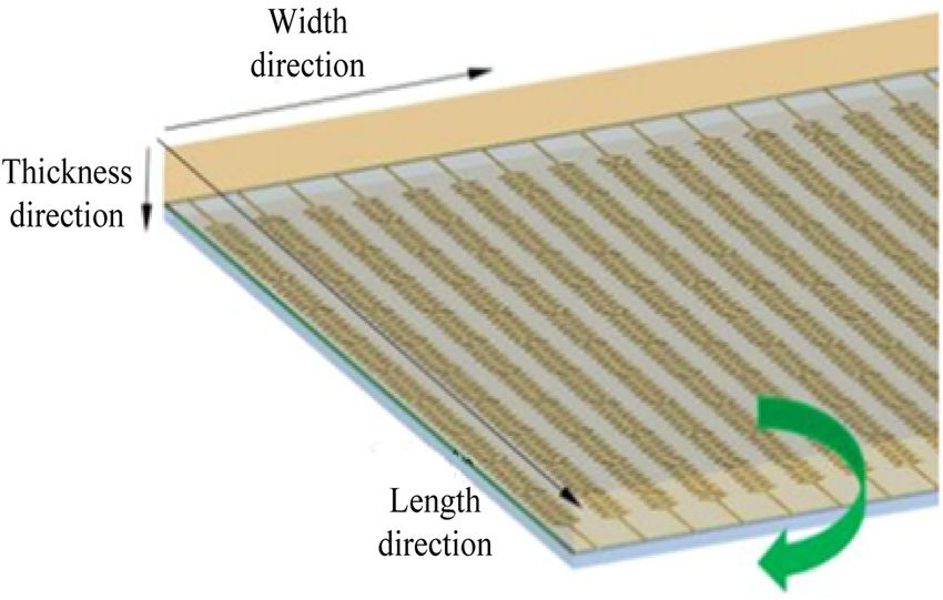
3D bending simulation and mechanical properties of the OLED bending area
←
→
Page content transcription
If your browser does not render page correctly, please read the page content below
Open Physics 2020; 18: 397–407
Research Article
Liang Ma* and Jinan Gu
3D bending simulation and mechanical
properties of the OLED bending area
https://doi.org/10.1515/phys-2020-0165 devices are attracting more and more attention [1]. People
received November 27, 2019; accepted May 30, 2020 have higher requirements with respect to power consump-
Abstract: Due to the poor mechanical properties of traditional tion, volume, softness, and other aspects of display devices.
simulation models of the organic light-emitting device (OLED) Display devices originated from cathode ray tubes (CRTs). In
bending area, this article puts forward a finite element model a CRT, electron flow bombards the screen, so that R, G, and
of 3D bending simulation of the OLED bending area. During B phosphors give out light in proportion, thus producing
the model construction, it is necessary to determine the different colors. Since the birth of the CRT technology in
viscoelastic and hyperelastic mechanical properties, respec- 1897, CRTs were applied in radar display and electronic
tively. In order to accurately obtain the stress changes of oscilloscopes at first, and then they were popularized in TVs
material deformation during the hyperelasticity determina- and computers, becoming the most mainstream display
tion, a uniaxial tensile test and a shear test were used to terminals in the twentieth century [2]. Although CRTs have
obtain data and thus to characterize the hyperelastic proper- strong advantages in terms of cost and image quality, their
ties. In order to measure the viscoelasticity, a stress relaxation weight, volume, radiation, and energy consumption limit
test was used to draw the stress relaxation curve, so as to their development. The dominant position of CRTs is
characterize the viscoelastic properties. Then, the plane or gradually replaced by flat panel displays (FPDs). Compared
axisymmetric stress–strain analysis was achieved, and the with the traditional CRTs, FPDs have many advantages,
material parameters of the 3D model of the OLED bending such as small size, light weight, and low energy consump-
area were obtained. Finally, the 3D model was applied to the tion. In recent years, FPDs have developed rapidly. Liquid
3D bending of the OLED bending area. Combined with the crystal displays (LCDs) and plasma display panels (PDPs)
axisymmetric finite element analysis method, the 3D bending are the most representative display devices. A pixel in an
simulation finite element model of the OLED bending area LCD panel is composed of three LCD units. Each LCD unit
was constructed by dividing the finite element mesh. contains a red filter, green filter, or blue filter. Different
Experimental results show that the mechanical properties of colors can be generated by controlling the light in different
the proposed model are better than those of traditional OLED units [3]. An LCD is thinner than a CRT, which greatly saves
bending simulation models. Meanwhile, the proposed model space and avoids the radiation problem. In the aspect of
has stronger application advantages. screen refresh rate, a CRT kinescope adopts light-emitting
materials. No matter how high the refresh frequency is, it
Keywords: OLED, bending area, 3D bending simulation, will lead to the flicker problem. Direct imaging technology
mechanical property for LCDs does not cause flicker, so it is more suitable for
human eyes. In addition, an LCD is a form of flat screen, and
the display effect is much better than that of a CRT.
1 Introduction However, LCDs also have some disadvantages in terms of
resolution, viewing angle, color saturation, brightness, and
With the rapid development of information age, the infor- reaction speed [4]. A pixel in a PDP is a plasma tube. The
mation display technology has become an important branch plasma gas discharges in the plasma tube, producing
of the information industry. As information carriers, display ultraviolet light and exciting the phosphor on the fluor-
escent screen. A PDP is a kind of self-luminous display
technology without backlight, which overcomes the pro-
* Corresponding author: Liang Ma, School of Mechanical
blems of visual angle and brightness of LCDs. It is easy to
Engineering, Jiangsu University, Zhenjiang 212000, China,
e-mail: maliang72@163.com
manufacture large-scale screens with excellent performance.
Jinan Gu: School of Mechanical Engineering, Jiangsu University, However, PDPs have some problems in terms of service life,
Zhenjiang 212000, China power consumption, and cost.
Open Access. © 2020 Liang Ma and Jinan Gu, published by De Gruyter. This work is licensed under the Creative Commons Attribution 4.0
Public License.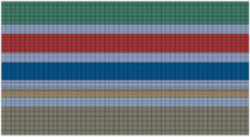
398 Liang Ma and Jinan Gu
Although LCDs, PDPs, and other displays solve the small, and the stress changes little with deformation.
problems of CRTs in terms of volume, weight, radiation, The measurement scheme is suitable for traditional
and screen refresh rate, they still need to be improved in hyperelastic materials, such as rubber, but it cannot be
the aspects of energy consumption, viewing angle, and completely suitable for the OCA material due to the
brightness. In recent years, LCDs and PDPs have been measurement accuracy. In order to accurately find the
unable to meet the growing demand for display stress changes during the material deformation, it is
functionality, especially flexible displays [5]. necessary to adopt appropriate instruments and mea-
The display of an organic light-emitting device surement schemes. For example, a uniaxial tensile test
(OLED) is thinner (its thickness is less than 500 nm), and a simple shear test are used to obtain data and thus
and it has the advantages of self-illumination, short to characterize the hyperelastic properties. When deter-
response time, large viewing angle, lifelike picture, high mining the viscoelasticity, we can use the stress
definition, and low energy consumption. It is a planar relaxation test to get the stress relaxation curve, so as
device and is highly compatible with plastic substrates. to characterize the viscoelastic properties. Thus, the
During its preparation, low-temperature technology is plane or axisymmetric stress–strain analysis is carried
adopted to achieve a flexible display. Compared with out [9].
other flexible displays, it has prominent advantages, as a
result of which it gradually became the first choice of
flexible displays. In addition, it is rated as the most 2.1.1 Determination and fitting of hyperelastic material
potential FPD lighting technology. However, an OLED parameters
display is a composite structure composed of thin-film
optical devices, and an optical clear adhesive (OCA) is The uniaxial tensile test and simple shear test were used
used to make the bonding of all film layers more firm to determine the hyperelasticity of materials. Dynamic
[6,7]. An OCA is a special adhesive used for cementing mechanical analysis (DMA) was applied to the uniaxial
transparent optical elements. It is required to have tensile test. A rotational rheometer was applied in the
colorless transparency, light transmittance above 90%, simple shear test.
good cementing strength, curing at room temperature or The thickness h of the specimens prepared by two
medium temperature, and curing shrinkage. In the tests is 1 mm. The measurement method is the same as
process of bending deformation, the bending radius of the viscoelastic measurement. The OCA samples are
flexible OLED modules is small. Meanwhile, various stacked and pasted, and then the specimens are cut as
thin-film devices cannot coordinate the deformation. The per the requirements of the chucking appliance [10].
OCA adhesive material has viscous flow, leading to Table 1 shows the size and instrument models of uniaxial
device stripping and permanent damage to the screen tensile specimens. Table 2 shows the specifications and
[8]. Therefore, a 3D bending simulation model of the instrument models of simple shear specimens. When
OLED bending area was built to research the mechanical DMA is adopted for the tensile test, the tensile rate refers
properties. to ASTM D412. When the rotary rheometer is adopted for
the simple shear test, the shear strain rate is 0.01 s−1.
The original data obtained from the experiment are
shown in Tables 1 and 2. After processing the data, we
2 Construction of a finite element can get the stress data and strain data. The specific
calculation is shown below.
model of 3D bending simulation In the uniaxial tensile test, the formula for proces-
of the OLED bending area sing stress σT and strain εT is as follows:
l − l0
εT = l
2.1 Parameter measurement and fitting of
0
, (1)
the OCA material σT = f
bh
An OCA is a kind of viscoelastic material. It is necessary where l0 is the original length of the specimen, l is the
to measure its viscoelastic and hyperelastic mechanical length of the specimen after stretching, f is the tensile
properties separately. In the determination of hypere- load, h is the thickness of the specimen, and b is the
lasticity, the elastic modulus of the OCA material is too tensile rate.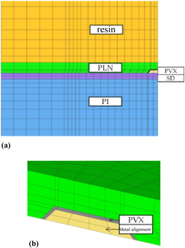
3D bending simulation and mechanical properties of OLED bending area 399
Table 1: Specimen size and instrument model of the uniaxial tension test
Serial number Instrument type DMA TA RSA-G2
1 Sample shape and size Long strip sample, l = 60 mm, B = 6 mm
2 Testing accuracy 0.02 mN
Table 2: Specimen size and instrument model of the simple shearing test
Serial number Instrument type Rotational rheometer TA DHR-2
1 Sample shape and size Disc specimen, radius r = 40 mm
2 Testing accuracy 0.01 mN
Simple tensile test
In the simple shearing test, the formula for proces-
Uniaxial fitting results
sing stress σS and strain γS is as follows: 0.04 Shear fit results
Simple shear experiment
rϕ 0.035
γS = h ,
(2)
σS = 2τ 0.03
πr 3
Nominal stress / MPa
0.025
where r is the torque of the parallel plate, φ is the
rotational displacement of the parallel plate, r is the 0.02
radius, and τ is the shear strain rate.
0.015
The stress and strain formulas of different strain
energy density function models under uniaxial tension 0.01
mode and simple shearing mode are obtained by
derivation. The derivation formulas are comparable 0.005
with experimental data, and the hyperelastic parameter
0
fitting can be achieved [1].
0 1 2 3 4
Through the mathematical software 1Stopt, the
Nominal strain / 100%
formula of stress–strain constitutive relation can be
derived. Combined with the experimental data, the Figure 1: Fitting results.
fitting results under different strain energy density
functions are obtained [11]. After the comparison of the an incompressible material, rather than a completely
fitting quality and the judgment of simulation conver- incompressible material in theoretical sense [13].
gence, the reduced polynomial model with N = 3 order is
adopted. The fitting results are shown in Figure 1.
We can see that the simple shear test data are 2.1.2 Determination and fitting of viscoelastic material
basically consistent with the simple shear fitting result. parameters
There is a slight difference between the data of the
uniaxial tensile test and the uniaxial tensile fitting results, DMA is applied to the viscoelastic stress relaxation test.
but they are consistent in the overall trend. On the whole, During the test, the specimens are prepared first. The
the fitting effect is very good. After the fitting, relevant thickness of specimens in the DMA test should not be less
parameters of the strain energy density function are than 1 mm, while the thickness of the OCA specimen should
obtained. The fitting parameters are shown in Table 3 [12]. be less than 0.05 mm. Therefore, it is necessary that the OCA
To be clear, the OCA material is an incompressible sample should be cemented, so that the thickness can reach
material. Poisson’s ratio v is 0.5. At this time, parameter D1 1 mm. Then, we cut the shape of specimens according to the
should be zero. In Abaqus, for materials whose Poisson’s requirements of fixtures and then we can obtain the
ratio v is greater than 0.475, Poisson’s ratio v is considered specimens for the experiments. The specification and
to be 0.475. That is to say, the material is approximated as instrument model are shown in Table 4.
400 Liang Ma and Jinan Gu
Table 3: Fitting parameters of the hyperelastic Yeoh model
Normalized
experimental data
0.8
Name Fitting parameters
Fitting result
C10 C20 C30 D1 D2 D3 0.7
Normalized relaxation modulus of elasticity
Numerical 0.01061 −0.00012 1.7318 4.79455 0 0 0.6
value × 10−6
0.5
Then, the simple shearing experiment is carried out. 0.4
A 5% instantaneous shear deformation is given to the
specimen. It is unchanged, and the change of stress is 0.3
recorded. The data are normalized using equation (3),
0.2
and then the data are input into Abaqus for fitting. The
result is shown in Figure 2 [14]. 0.1
N
g (t ) = 1 − ∑ gi(1 − e−t /τ ),
i (3) 0
0 50 100 150 200
i=1
Time /s
where g(t) is the relaxed modulus of elasticity after
Figure 2: Fitting results.
normalization, t is the relaxation time, N is the number
of terms of the Prony series, gi and τi are the parameters
in the model, e is the shear threshold, and i is a constant. Table 5: Prony parameters based on viscoelastic fitting
For the viscoelastic fitting process of the material, it is
only necessary to nondimensionalize the experimental data i 1 2 3 4 5
of stress relaxation in Abaqus, and thus to achieve the plane
gi 0.5902 0.1461 0.1115 0.0643 0.0352
or axisymmetric stress–strain analysis. After input, Prony τi 0.0188 0.2084 1.8675 19.167 233.07
parameters gi and τi can be obtained by fitting. Finally, the
viscoelastic properties are given to the materials.
It can be seen that the fitting curve basically wiring at the end of the bending area is used to transmit
coincides with the experimental data curve after the and control the electric signal of the light-emitting diodes
normalization. The fitting quality is very good. After in the OLED display area. There are huge amounts of metal
fitting, Prony parameters gi and τi are obtained (Table 5). wires deposited in the organic photoresist [15]. The
structure of the bending area is shown in Figure 3.
According to the structural characteristics of the
OLED bending area, OCA material parameters and
2.2 Construction of the 3D model of the membrane material parameters are obtained. The OCA
OLED bending area material parameters are shown in Figure 4.
The parameters of membrane materials are shown in
2.2.1 Material parameters Table 6.
The structure of the OLED bending area is mainly 2.2.2 Construction of the 3D model
composed of an organic photoresist, metal wiring, and a
polyimide (PI) substrate. The metal wiring at the end of the In order to simplify the OLED bending area, meso-
structure is deposited in the organic photoresist. The metal structure information is introduced to characterize the
Table 4: Specimen size and instrument model
Serial number Instrument type DMA TA RSA-G2
1 Sample shape and size Long strip sample, l = 50 mm, B = 5 mm
2 Testing accuracy 0.01 mN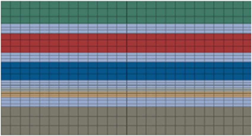
3D bending simulation and mechanical properties of OLED bending area 401
Table 6: Parameters of membrane materials
Back panel material Modulus of Poisson’s ratio
elasticity (GPa)
Protective cover 5.6 0.29
plate
Touch layer 4.076 0.31
Polarizer 3.769 0.33
Display layer 49 0.30
Substrate 9.1 0.33
Backplane 4.2 0.32
Figure 3: Structure of the OLED bending area.
Protective cover plate-60 µm
OCA-25 µm
Figure 5: 3D model of the bending area.
Touch layer-50 µm
OCA-25 µm Table 7: Geometric parameters
Polarizer-47 µm
Serial number Material layer Thickness (µm)
OCA-20 µm
1 Organic photoresist 4.5
Display layer-10 µm
2 Metal alignment 0.73
Substrate-15 µm
3 Substrate material 1.5
OCA-25 µm 4 PI substrate 15
Backplane-75 µm
For the 3D model of the bending area, the geometric
parameters of relevant metal lines and material layers
Figure 4: OCA rubber parameters. are shown in Table 7.
properties of the bending area. The micromechanics of
materials are based on the relationship between the
macromechanical properties of materials and the micro- 2.3 Construction of the finite element
structure. Therefore, the macroproperties can be model of 3D bending simulation of the
achieved by optimizing the design of the microstructure. OLED bending area
The structure region at the end of the OLED has obvious
periodic characteristics [16]. According to the character- 2.3.1 3D bending for the OLED bending area
ization of the microstructure, the microstructure of the
end structure of the OLED can be composed of an The 3D model of the OLED bending area is combined
organic photoresist, single metal wire, substrate mate- with the axisymmetric principle, and the OLED bending
rial, and PI substrate. Thus, the 3D model of the bending area is bent in the 3D mode, so that the lower part of the
area is built as shown in Figure 5. screen is able to fit with the middle frame. Thus, the
402 Liang Ma and Jinan Gu
150
screen
Reference Rigid
point body
Figure 6: Bending structure and size.
screen rotation is achieved. The middle frame can be
regarded as a rigid body. In order to form a circular arc at
the bending part and reduce the structure stress, the
distance between the reference point and the symmetry axis
π
is set as 4 R mm . When R is 5 mm, the distance is 7.85 mm.
The structure and size are shown in Figure 6 [17].
Figure 8: 3D bending simulation model of the OLED bending area.
In the first second, the rigid body rotates antic-
lockwise around the reference point, at a speed of
1.57 rad/s. At the same time, the rigid body moves to the After bending, the 3D bending simulation model of the
π OLED bending area is built as shown in Figure 8.
left at a speed of 4 − 1 R mm. The shape after bending
is shown in Figure 7. After that, it is placed for 300 s to
simulate the actual use. 2.3.2 Grid partition based on axisymmetric finite
When the bending radius R = 5 mm, the boundary element analysis
condition is that in the first second, the rigid body
rotates anticlockwise around the reference point at a According to the 3D bending simulation model of
speed of 1.57 rad/s, and then it moves to the left at a the OLED bending area, the finite element model of
speed of 2.85 mm/s. Finally, it is placed for 300 s. the three-dimensional bending process is built. First, the
axisymmetric finite element analysis method is used to
generate the finite element meshes. After bending, the
difference between the internal metal wiring width in the
OLED bending area and the overall size is large. It is
more difficult to generate finite element meshes [18]. It is
easy to ignore some characteristics of the metal wiring
screen Rigid
body structure by using the whole grid division method,
influencing the analysis of different metal wiring
structures negatively. It is not able to reflect the
structural differences of different metal wires. Combined
with the principle of axisymmetric finite element
R5 analysis, the implicit dynamic viscoelastic analysis
method was adopted for the grid division. In order to
be consistent with the actual stress situation, the plane
Reference
point strain grids are adopted. During the mesh generation,
the network is quadrilateral, which is convenient for
convergence and calculation. The grid size is 0.025 mm.
All the membrane materials and OCA materials are
divided into three layers. The grid type includes the
plane strain unit, hybrid unit, and CPE8RH reduced
integration unit.
A HyperMesh platform with powerful finite element
Figure 7: Shape after bending. preprocessing ability is used for the OLED bending area.3D bending simulation and mechanical properties of OLED bending area 403
A hexahedron mesh method is used to divide the metal
wires and other areas. This can effectively reduce the
number of meshes. On this basis, progressive grid
division is adopted to ensure the accuracy of the
calculated structure and thus to reduce the calculation
time. All units in the model are linear hexahedron
elements with complete integration [19].
Generally, the accuracy of grid division directly influ-
ences the accuracy of the result. The finer the mesh division
is, the more accurate the result is. When the grid is too dense,
the computer overhead will increase and the computing time
will also increase. For the explicit dynamics, the consumption Figure 10: Finite element meshes after the detailed division.
of computer memory and computing time are directly
proportional to the number of grid units. The computing The details of the division of finite element meshes after
cost increases with the improvement of grid subdivision, so the OLED bending are shown in Figure 11.
that we can directly predict the cost change caused by grid
subdivision. For the implicit dynamics, the computing cost is
roughly proportional to the square of the number of freedom 2.3.3 Finite element modeling
degrees. The consumption of memory and computing time
will have an exponential relationship with the number of grid Refined finite element meshes are used to build the
units. It is difficult to predict the cost. The change is obvious. three-dimensional bending simulation finite element
On the basis of accuracy, a reasonable grid density can model of the OLED bending area. During the finite
greatly optimize the computing cost. For the structure of
the OLED bending area, on the premise of reflecting the
structural features of the metal wire, we must refine the grid
as much as possible, so that the grid size can ensure the
computing accuracy without consuming too much com-
puting resource [20]. Due to the ratio of the length and
thickness of the OLED bending area after bending, the
number of metal wiring meshes is still huge on the basis of
accuracy, consuming too much computer resource. In order
to improve the accuracy of calculation and analysis, a sub-
model is used to divide the structure of the OLED bending
area after bending. There are 26 × 30 divided finite element
grids, as shown in Figure 9.
On this basis, the finite element meshes are divided
in detail. The specific results are shown in Figure 10.
Figure 11: Details of the finite element mesh after the detailed
Figure 9: Finite element mesh. division: (a) details of finite element mesh and (b) enlarged details.404 Liang Ma and Jinan Gu
element simulation, the setting of boundary condition load
directly influences the success of simulation. This is also
an extremely important part of finite element simulation.
In the finite element simulation, there are two ways to Global boundary
conditions
realize the periodic boundary: (1) coupling corre-
sponding surface nodes. This method has higher
requirements for serial number of nodes, but it can
reduce constraints and improve calculation accuracy. (2)
A penalty function is introduced. The implementation of
this method is simple, but it is easy to cause a numerical
difference. Therefore, the periodic boundary constraints
can be achieved by combining these two methods. The
special boundary constraint needs to divide the whole z
model into two independent models: a global model and
a sub-model. The global model includes a geometric x
constraint, displacement constraint, and boundary con-
y
straint. The sub-model is a part of the whole model, so
we cannot analyze the global features of the model, such
as cracks. In the global model, the displacement
corresponding to the sub-model is the boundary condi- load
tion of the sub-model. Therefore, the grid of the global
model is relatively coarse. If the global model corre- Figure 12: Global model.
sponds to the sub-model, the calculation results will be
more accurate [21].
bending speed is expanded n times, the calculation time will
The basic implementation steps of special boundary 1
be shortened to n of the original time. In order to ensure that
constraints in the finite element analysis include the
following: the energy distribution in the simulation process is
(1) global model analysis: the global model is divided consistent with the actual situation, the simulation speed
with coarse meshes without considering the local should be stable. Therefore, the bending speed is set as
structure details, and then the global structure is 3,000 mm/s, the optimal bending radius is 2 mm, and the
analyzed to calculate the displacement at a specific time to complete the simulation is 2.444 s. Then, the
location (near the boundary of the sub-model). amplitude curve of finite element analysis is obtained. The
(2) establishment of the sub-model: according to the specific process is shown in Figure 14.
analysis target and the actual structure, the sub-
model of a local fine mesh is built.
(3) boundary condition interpolation value: the displa- Sub boundary conditions / loads
cement boundary of the global model obtained in
the first step is taken as the boundary condition.
Then, it is automatically loaded to the corresponding
position in the sub-model by the linear interpolation
method (the displacement interpolation result de-
termines the computing accuracy of the sub-model).
(4) result analysis of the sub-model: the original
boundary and load in the region of sub-models are
unchanged, and then the finite element analysis is
performed on sub-models. The global model is shown z
in Figure 12, and the sub-model is shown in Figure 13.
x
In the setting of boundary conditions, the efficiency of y
calculation can be improved by increasing the bending
speed under the condition of a constant time step. If the Figure 13: Sub-model.3D bending simulation and mechanical properties of OLED bending area 405
Table 8: Parameters of each material layer in the finite element
model
Open. DXF format file
Material layer Young’s Poisson’s ratio
modulus (Mpa)
PI substrate 9,200 0.35
Organic photoresist 3,400 0.35
Read. DXF format file Metal alignment 80,000 0.35
Inorganic substrate 1,10,000 0.17
According to the amplitude curve of finite element
analysis, HyperMesh software is used to build the finite
Calculate interpolation
Enter sample interval element model of three-dimensional bending simulation
point value
of the OLED bending area. The specific model is shown
in Figure 15.
Enter bending speed
Calculating displacement 3 Research on mechanical properties
array
3.1 Experimental process
The mechanical properties in the bending process of the
Get the amplitude curve of OLED bending area were researched using the 3D
Input channel spacing
finite element analysis
compress stretching
Figure 14: Specific process of obtaining the amplitude curve of finite
element analysis.
Protective cover plate 60 µm
OCA1 25 µm
Touch layer 50 µm
OCA2 25 µm
Polarizer 47 µm
OCA3 20 µm
Display layer 10 µm
Substrate 15 µm
OCA4 25 µm
Backplane-75 µm
-0.02 -0.015 -0.01 -0.005 0 0.005 0.01 0.015 0.02
Nominal strain / 100%
Periodic boundary condition algorithm
Special boundary constraints
Bending mechanical response
Figure 15: Finite element model of 3D bending simulation of the Figure 16: Experimental results of mechanical properties of
OLED bending area. traditional models.406 Liang Ma and Jinan Gu
compress stretching
Protective cover plate 60 µm
OCA1 25 µm
Touch layer 50 µm
OCA2 25 µm
Polarizer 47 µm
OCA3 20 µm
Display layer 10 µm
Substrate 15 µm
OCA4 25 µm
Backplane-75 µm
-0.02 -0.015 -0.01 -0.005 0 0.005 0.01 0.015 0.02
Nominal strain / 100%
Periodic boundary condition algorithm
Special boundary constraints
Bending mechanical response
Figure 17: Experimental results of mechanical properties of the proposed model.
bending simulation finite element model of the OLED mechanical properties of three traditional OLED bending
bending area [22–25]. First, the material parameters of simulation models are shown in Figure 16.
each layer in the finite element model were calculated. The experimental results of the mechanical properties of
The specific results are shown in Table 8. the finite element model of three-dimensional bending
In order to ensure the fairness and effectiveness of simulation of the OLED bending area are shown in Figure 17.
the experimental results, three traditional bending According to the verification results of mechanical
simulation models such as the model based on a periodic properties, the performance of strain distribution of the
boundary condition algorithm, the model based on finite element model of three-dimensional bending
special boundary constraints, and the model based on simulation of the OLED bending area is better than
bending mechanical response were used to compare the that of the traditional model, so that the effectiveness of
finite element model designed in this article. The the proposed model can be proved.
mechanical properties of the proposed model were
judged using the strain distribution [26,27]. The more
tortuous the strain distribution curve is, the stronger the
strain distribution performance is. 4 Conclusions
Due to the poor mechanical properties obtained in the
traditional simulation models of the OLED bending area,
3.2 Research results a finite element model for three-dimensional bending
simulation of the OLED bending area is proposed. This
In this study, the mechanical properties of the bending model effectively improves the mechanical properties, so
region were analyzed by observing the motion states at it has great significance for the research on the bending
different positions. The experimental results of the properties of OLED screens.3D bending simulation and mechanical properties of OLED bending area 407
References the rotating motor protein F 1 F 0 -ATP synthase. Proc Natl
Acad Sci. 2017;114(43):11291–6.
[1] Siemowit M, Małgorzata K, Ewa T, Izabela Ś, Piotr D, Kornel K, et al. [14] Wang Z, Su F, Zhang X, Yan S, Zhang ZM. Effect of transverse
Effect of caponization on performance and quality characteristics of position and numbers on the stability of the spinal pedicle
long bones in Polbar chickens. Poult Sci. 2017;96(2):491–500. screw fixation during the pedicle cortex perforation. Chin Med
[2] Zhang W, Ma QS, Dai KW, Mao WG. Fabrication and properties Sci J. 2017;39(3):365–70.
of three-dimensional braided carbon fiber reinforced SiOa- [15] Chadefaux D, Rao G, Carrou JLL, Berton E, Vigouroux L. The
rich mullite composites. J Wuhan Univ Technol-Mater Sci Ed. effects of player grip on the dynamic behaviour of a tennis
2019;34(4):798–803. racket the effects of player grip on the dynamic behaviour of a
[3] Tang YD, Huang BX, Dong YQ, Wang WL, Zheng X, Zhou W, tennis racket. J Sports Sci. 2017;35(12):1155–64.
et al. Three-dimensional prostate tumor model based on a [16] Grubb MP, Coulter PM, Marroux HJB, Orr-Ewing AJ,
hyaluronic acid-alginate hydrogel for evaluation of anti-cancer Ashfold MNR. Unravelling the mechanisms of vibrational
drug efficacy. J Biomater Sci Polym Ed. 2017;28(14):1–23. relaxation in solution. Chem Sci. 2017;8(4):3062–9.
[4] Lin DC, Zhao J, Sun J, Yao HB, Liu YY, Yan K, et al. Three- [17] Sun Z, Zhao W, Kong DJ. Microstructure and mechanical
dimensional stable lithium metal anode with nanoscale property of magnetron sputtering deposited DLC film. J Wuhan
lithium islands embedded in ionically conductive solid matrix. Univ Technol (Mater Sci Ed). 2018;33(3):579–84.
Proc Natl Acad Sci USA. 2017;114(18):4613–8. [18] Meng XK, Zhao CW. Effect of Dy addition on the microstructure
[5] Li JZ, Xue F, Blu T. Fast and accurate three-dimensional point and mechanical property of Ti-Nb-Dy alloys. J Wuhan Univ
spread function computation for fluorescence microscopy. Technol-Mater Sci Ed. 2019;34(4):940–4.
J Opt Soc Am A Opt Image Sci Vis. 2017;34(6):1029–34. [19] Helma C, Cramer T, Kramer S, Raedt LD. Data mining and
[6] Fujita T. Hierarchical nanoporous metals as a path toward the machine learning techniques for the identification of muta-
ultimate three-dimensional functionality. Sci Technol Adv genicity inducing substructures and structure activity rela-
Mater. 2017;18(1):724–40. tionships of noncongeneric compounds. J Chem Inf Comput
[7] Saxena P, Gorji NE. COMSOL simulation of heat distribution in Sci. 2004;44(4):1402–11.
perovskite solar cells: coupled optical-electrical-thermal 3-D [20] Ge SB, Wang LS, Liu ZL, Jiang SC, Yang XX, Yang W, et al.
analysis. IEEE J Photovolt. 2019;9(6):1693–8. Properties of nonvolatile and antibacterial bioboard produced
[8] Han YC, Jeong EG, Kim H, Kwon S, Gyun H, Baeb BS, et al. from bamboo macromolecules by hot pressing. Saudi J Biol
Reliable thin-film encapsulation of flexible OLEDs and Sci. 2017;25(3):474–8.
enhancing their bending characteristics through mechanical [21] Yang M, Li J, Xie WF. Preparation, antibacterial and antistatic
analysis. RSC Adv. 2016;6(47):40835–43. properties of PP/Ag-Ms/CB composites. J Wuhan Univ Technol
[9] Chieko M, Toshio I, Toshitsugu K. Adhesion of human (Mater Sci Ed). 2018;33(3):749–57.
periodontal ligament cells by three-dimensional culture to the [22] Ahmad Y, Ali U, Bilal M, Zafar S, Zahid Z. Some new standard
sterilized root surface of extracted human teeth. J Oral Sci. graphs labeled by 3-total edge product cordial labeling. Appl
2017;59(3):365–71. Math Nonlinear Sci. 2017;2:61–72.
[10] Uchida Y, Motoyoshi M, Namura Y, Shimizu N. Three- [23] Attia GF, Abdelaziz AM, Hassan IN. Video observation of
dimensional evaluation of the location of the mandibular perseids meteor shower 2016 from Egypt. Appl Math
canal using cone-beam computed tomography for orthodontic Nonlinear Sci. 2017;2:151–6.
anchorage devices. J Oral Sci. 2017;59(2):257–62. [24] Bortolan MC, Rivero F. Non-autonomous perturbations of a
[11] Regmi P, Nelson N, Haut RC, Orth MW, Karcher DM. Influence non-classical non-autonomous parabolic equation with sub-
of age and housing systems on properties of tibia and critical nonlinearity. Appl Math Nonlinear Sci. 2017;2:31–60.
humerus of lohmann white hens: bone properties of laying [25] Dewasurendra M, Vajravelu K. On the method of inverse
hens in commercial housing systems. Poult Sci. mapping for solutions of coupled systems of nonlinear
2017;96(10):3755–62. differential equations arising in nanofluid flow, heat and mass
[12] Wu JF, Lu CL, Xu XH, Zhang YX, Wang DB, Zhang QK. Cordierite transfer. Appl Math Nonlinear Sci. 2018;3:1–14.
ceramics prepared from poor quality kaolin for electric heater [26] Gao W, Zhu L, Guo Y, Wang K. Ontology learning algorithm for
supports: sintering process, phase transformation, micro- similarity measuring and ontology mapping using linear
structure evolution and properties. J Wuhan Univ Technol- programming. J Intell Fuzzy Syst. 2017;33:3153–63.
Mater Sci Ed. 2018;33(3):598–607. [27] Gao W, Wang WF. The fifth geometric-arithmetic index of
[13] Almendrovedia V, Natale P, Mell M, Bonneau S, Monroy F, bridge graph and carbon nanocones. J Differ Equ Appl.
Joubert F. Nonequilibrium fluctuations of lipid membranes by 2017;23:100–9.You can also read