Numerical Investigation of Surge Waves Generated by Submarine Debris Flows
←
→
Page content transcription
If your browser does not render page correctly, please read the page content below
water
Article
Numerical Investigation of Surge Waves Generated by
Submarine Debris Flows
Zili Dai, Jinwei Xie, Shiwei Qin * and Shuyang Chen

                                          Department of Civil Engineering, Shanghai University, 99 Shangda Road, Shanghai 200444, China;
                                          zilidai@shu.edu.cn (Z.D.); xiejinwei0828@163.com (J.X.); chenshuyangsusie@163.com (S.C.)
                                          * Correspondence: 10002358qsw@shu.edu.cn; Tel.: +86-18817879593

                                          Abstract: Submarine debris flows and their generated waves are common disasters in Nature that
                                          may destroy offshore infrastructure and cause fatalities. As the propagation of submarine debris
                                          flows is complex, involving granular material sliding and wave generation, it is difficult to simulate
                                          the process using conventional numerical models. In this study, a numerical model based on the
                                          smoothed particle hydrodynamics (SPH) algorithm is proposed to simulate the propagation of
                                          submarine debris flow and predict its generated waves. This model contains the Bingham fluid
                                          model for granular material, the Newtonian fluid model for the ambient water, and a multiphase
                                          granular flow algorithm. Moreover, a boundary treatment technique is applied to consider the
                                          repulsive force from the solid boundary. Underwater rigid block slide and underwater sand flow
                                          were simulated as numerical examples to verify the proposed SPH model. The computed wave
                                          profiles were compared with the observed results recorded in references. The good agreement
                                          between the numerical results and experimental data indicates the stability and accuracy of the
                                          proposed SPH model.

                                   Keywords: submarine debris flow; surge wave; smoothed particle hydrodynamics; water–soil
Citation: Dai, Z.; Xie, J.; Qin, S.;      interface; multiphase flow
Chen, S. Numerical Investigation of
Surge Waves Generated by
Submarine Debris Flows. Water 2021,
13, 2276. https://doi.org/10.3390/        1. Introduction
w13162276
                                               Submarine debris flows are widely distributed on continental shelves, continental
                                          slopes and in deepwater areas, where they pose a serious threat to offshore infrastructure,
Academic Editor: Giuseppe Pezzinga
                                          such as submarine pipelines and cables, offshore oil and gas platforms, and offshore
                                          wind farms [1]. In addition, submarine debris flows can generate huge surge waves that
Received: 4 July 2021
Accepted: 18 August 2021
                                          can seriously threaten the safety of infrastructure and people living in coastal areas. For
Published: 20 August 2021
                                          example, the 1958 Lituya Bay debris flow-generated tsunami produced a run-up of over 400
                                          m [2]. Another significant tsunami was generated by a submarine debris flow at the Nice
Publisher’s Note: MDPI stays neutral
                                          airport in France on 16 October 1979, and swept away 11 people [3]. The 1994 Skagway
with regard to jurisdictional claims in
                                          debris flow-generated tsunami destroyed a railway dock, damaged the harbor, and killed a
published maps and institutional affil-   construction worker in Alaska, USA [4,5]. A submarine debris flow in Papua New Guinea
iations.                                  generated a wall of water measuring 15 m high that killed over 2100 people in July 1998 [6].
                                          Furthermore, the 2006 Java tsunami, generated by a submarine debris flow off of Nusa
                                          Kambangan Island, produced a run-up in excess of 20 m at Permisan [7]. In 2010, the slope
                                          failures of river deltas along the Haitian coastline triggered tsunamis with a height of 3 m,
Copyright: © 2021 by the authors.
                                          which caused at least three fatalities and some damage to infrastructure [8]. In 2018, the
Licensee MDPI, Basel, Switzerland.
                                          submarine debris flow induced by the Palu earthquake resulted in devastating tsunamis
This article is an open access article
                                          and caused more than 2000 fatalities in Sulawesi, Indonesia [9–11]. These debris flow-
distributed under the terms and           generated tsunami disasters have therefore attracted a lot of attention from researchers.
conditions of the Creative Commons             Catastrophic tsunami waves generated by submarine debris flows are difficult to
Attribution (CC BY) license (https://     observe and record because of their inaccessibility and unpredictability. Current approaches
creativecommons.org/licenses/by/          to investigating the surge waves generated by submarine debris flows mainly focus on
4.0/).                                    physical model tests and numerical simulations. For instance, physical model tests were

Water 2021, 13, 2276. https://doi.org/10.3390/w13162276                                                      https://www.mdpi.com/journal/water
Water 2021, 13, 2276                                                                                         2 of 13

                       conducted based on the generalized Froude similarity to study the complex wave patterns
                       generated by debris flows at Oregon State University [12]. Later, McFall and Fritz [13]
                       conducted physical modeling using gravel and cobble materials in different topographic
                       conditions, and analyzed offshore tsunami waves. Wang et al. [14] conducted physical
                       model tests to analyze the effect of volume ratio on the maximum tsunami amplitude,
                       and obtained an optimization model to predict the maximum tsunami amplitude. Miller
                       et al. [15] designed a large flume model test to measure the shape and amplitude of the
                       near-field waves and investigate the fraction of debris flow mass that activates the leading
                       wave. Meng [16] conducted a series of model tests to investigate the waves generated by
                       debris flow at laboratory scale, and the effect of the sliding mass on the wave features was
                       analyzed. Takabatake et al. [17] conducted subaerial, partially submerged, and submarine
                       debris flow-generated tsunamis to investigate the different characteristics of these three
                       types of tsunamis. Although some promising results have been obtained, the physical
                       model tests conducted in the abovementioned work require a great deal of manpower
                       and material resources. In addition, the size effect is an inevitable problem in physical
                       modeling.
                             With the rapid development of computer techniques and numerical algorithms, nu-
                       merical modeling of such events is critical to better understand the mechanism of surge
                       waves and predict their propagation behavior, and become more prevalent in recent
                       years. For example, Lynett and Liu [18] derived a numerical model to simulate the waves
                       generated by a submarine debris flow and to predict the run-up. Yavari–Ramshe and
                       Ataie–Ashtiani [19] presented a comprehensive review on past numerical investigations of
                       debris flow-generated tsunami waves. In this review study, numerical models based on
                       depth-averaged equations (DAEs) were tabulated according to their conceptual, mathemati-
                       cal, and numerical approaches. Recently, a novel multiphase numerical model based on the
                       moving particle semi-implicit method was proposed and applied to simulate submerged
                       debris flows and tsunami waves. The model was validated and evaluated through compar-
                       ison with the experimental data and other numerical models [20]. Sun et al. [21] solved the
                       Navier–Stokes equations and incompressible flow continuity equation and developed a
                       numerical model to investigate the propagation of a debris flow-generated tsunami under
                       different initial submergence conditions. Rupali et al. [22] developed a coupled model
                       based on the boundary element method and spectral element method to describe the char-
                       acteristics of debris flow-generated waves. Baba et al. [23] adopted a two-layer flow model
                       to simulate the submarine mass movement and surged wave propagation. In addition,
                       computational fluid dynamics (CFD) has been widely applied to analyze tsunami wave
                       propagation [24,25]. In the field of CFD, a mesh-free particle method named smoothed
                       particle hydrodynamics (SPH) was proposed as an astrophysics application and has been
                       widely used in various engineering fields [26]. For example, Iryanto [27] established an
                       SPH model to simulate the waves induced by aerial and submarine landslides. Wang
                       et al. [28] proposed a coupled DDA–SPH model to deal with the solid–fluid interaction
                       problem, and applied it to simulate a block sliding along an underwater slope. However,
                       the landslide mass was simulated as a rigid body, and its deformation was neglected in
                       these two models. This work aimed to establish an SPH model to simulate surge waves
                       generated by submarine debris flows, and to show the accuracy and stability of this model
                       in the simulation of multiphase flow problems.

                       2. Materials and Methods
                       2.1. SPH Algorithm
                            The SPH method was proposed in 1977 for astrophysical applications [29]. Recently,
                       this method has been widely applied to a large variety of engineering fields [30–33].
                       Compared to the mesh-based methods, the major advantage of this method is that it
                       bypasses the need for numerical meshes and avoids the mesh distortion issue and a great
                       deal of computation for mesh repartition [34].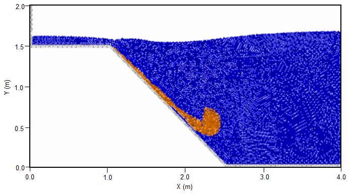
Water 2021, 13, 2276                                                                                             3 of 13

                            In the SPH method, the governing equations can be transformed from partial dif-
                       ferential equation form into SPH form by two approximation methods. The first one is
                       to produce the functions using integral representations, which is usually called kernel
                       approximation. The second one is to discretize the problem domain into a set of particles,
                       which is called particle approximation. Based on these two approximations, field variables
                       and their derivative in SPH form can be expressed by the following equations [35]:

                                                                  N   m j f xj
                                                      f ( xi ) ≈ ∑

                                                                                 W xi − x j , h                     (1)
                                                                 j =1
                                                                          ρj

                                                                  N m f x       ∂W xi − x j , h
                                                  ∂ f ( xi )         j    j
                                                             ≈ −∑             ·                                     (2)
                                                    ∂xi         j =1
                                                                       ρj           ∂xi

                       where f is an arbitrary field function, x is the coordinates of the SPH particles, m is the mass
                       of particles, ρ is the density, W is the smoothing function, h is the smoothing length, and N
                       is the total number of neighboring particles.

                       2.2. Governing Equations
                            In the presented model, soil and water in a large deformation situation are assumed
                       as two different fluids that occupy the space by a certain volume fraction. They satisfy the
                       conservation law of mass and momentum, respectively [36]:

                                                              1 D (ρes φs )
                                                                            + φs ∇ · ves = 0                        (3)
                                                             ρes   Dt

                                                           1 D (ρew φw )
                                                                         + φw ∇ · vew = 0                           (4)
                                                         ρew     Dt
                                                             De
                                                              vs   1               1
                                                        φs       = ∇σ e s + φs g + fs                               (5)
                                                             Dt   ρes             ρes
                                                           De
                                                            vw     1                 1
                                                      φw       =     ∇σ
                                                                      e w + φw g +     f                            (6)
                                                           Dt    ρew               ρew s
                       where t is the time, g is the gravitational acceleration. v denotes the velocity vector, and
                       σ denotes the stress tensor. The subscripts w and s represent water and soil, respectively.
                       Moreover, ϕs and ϕw are the volume fractions of soil and water, and fs is the force exerting
                       on the soil by the water, which can be determined by:

                                                                  fs = −φs ∇ p + fd                                 (7)

                       where f d is the Darcy penetrating force, and p is the pressure term of the fluid, which is
                       calculated by an equation of state [37]:

                                                                      ρ0 c2s
                                                                                       γ
                                                                                    ρ
                                                              p=                              −1                    (8)
                                                                       γ            ρ0

                       where ρ0 is the reference density, which can be measured through laboratory tests; ρ is the
                       density obtained through the mass conservation equation; cs is the sound speed, which can
                       be set equal to ten times the maximum velocity [38]; and γ is the exponent of the equation
                       of state, and is usually set to 7.0 [39].

                       2.3. Material Model
                            In the presented SPH model, the submarine debris flow is assumed to be a Bingham
                       viscous fluid, and the relationship between the shear stress and the shear strain rate is
                       defined as:
                                                                   .
                                                             τ = η γ + τy                                    (9)
2.3. Material Model
In the presented SPH model, the submarine debris flow is assumed to be a Bingham
viscous fluid, and the relationship between the shear stress and the shear strain rate is
defined as:
Water 2021, 13, 2276 4 of 13
τ = ηγ + τ y (9)
where τ denotes the shear stress, η represents the viscosity coefficient in fluid dynamics,
.
γ means
where the shear
τ denotes thestrain
shearrate, and
stress, τy is the Bingham
η represents yield stress.
the viscosity coefficient in fluid dynamics, γ
means the
The shear strain
ambient waterrate, and τ y isasthe
is assumed BinghamNewtonian
a classical yield stress.fluid, and the deformation
The can
behavior ambient water isas:
be described assumed as a classical Newtonian fluid, and the deformation
behavior can be described as:
τ =ηγ.
τ = ηγ (10)
(10)
The
The viscosity
viscosity of
of water
water ηη is
is 1.7
1.7 ××10
10−Pa·s.
−3 3
Pa·s.
2.4.
2.4. Approach
Approach for for Multiphase
Multiphase Granular
Granular Flow
Flow Modeling
Modeling
In
In this SPH model, the approach for multiphase granular
this SPH model, the approach for multiphase granular flow
flow proposed
proposed by by Tajnesaie
Tajnesaie
et
et al. [20] is
is adopted.
adopted.As Asshown
shownininFigure
Figure 1, 1,
thethe debris
debris flowflow is represented
is represented by granular-
by granular-type
type (in brown
(in brown color)color) particles,
particles, and the and the iswater
water is represented
represented by fluid-type
by fluid-type (in blue
(in blue color) color)
particles.
particles. As the flow
As the granular granular flow
is quite is quite
fast, and thefast, and the permeability
permeability is low, it isisassumed
low, it isinassumed
this modelin
thatmodel
this the massthatexchange
the mass between
exchangethe ambient
between theand pore and
ambient water is negligible.
pore Each particle
water is negligible. Each
has its own
particle has physical and mechanical
its own physical properties.
and mechanical The fluid-type
properties. particles particles
The fluid-type are regarded as
are re-
Newtonian fluid, and the viscosity is constant. In contrast, the granular-type
garded as Newtonian fluid, and the viscosity is constant. In contrast, the granular-type particles are
regardedare
particles as Bingham
regarded viscous
as Binghamfluid,viscous
and thefluid,
viscosity is variable
and the viscosityand determined
is variable and by the
deter-
rheological
mined by the model, as described
rheological model,in asSection
described2.3.in Section 2.3.
Figure
Figure 1.
1. Particle
Particle representation
representation of
of multiphase
multiphase granular
granular continuum.
continuum.
2.5. Treatment
2.5. Treatment on
on Water–Soil
Water–Soil Interface
Interface
As shown
As shownin inFigure
Figure2a,
2a,density
densityand
and mass
mass areare discontinuous
discontinuous nearnear
thethe water–soil
water–soil in-
interface, reducing the computational accuracy and stability when solving the governing
Water 2021, 13, x FOR PEER REVIEW terface, reducing the computational accuracy and stability when solving the governing 5 of 15
equations. Therefore,
equations. Therefore, boundary
boundary treatments
treatments on
on the
the water–soil
water–soil interface
interface should
should be
be made
made
when solving the governing equations.
when solving the governing equations.
As shown in Figure 2a, a is the central particle (in red) and b represents the neighbor-
ing particles of the other phase (in yellow). In this model, particle b is converted into par-
ticle b' (in blue) of the same phase with particle a, as shown in Figure 2b, which occupies
the same position, velocity, and volume as the original particle b. Only the position, vol-
ume, velocity, and pressure of these neighboring particles are taken into account in parti-
cle approximation.
(a) (b)
Figure
Figure2.2.Treatment
Treatmenton
onthe
theinterface
interfaceof
ofdifferent
differentfluids:
fluids:(a)
(a)original
originalparticles;
particles;(b)
(b)converted
convertedparticles.
particles.
As shown
2.6. Boundary in Figure 2a, a is the central particle (in red) and b represents the neighboring
Condition
particles of the other phase (in yellow). In this model, particle b is converted into particle
During the submarine debris flow propagation, the fluid particles face resistance
b’ (in blue) of the same phase with particle a, as shown in Figure 2b, which occupies the
from the local seabed. Therefore, to truly simulate the debris flow motion, it is important
same position, velocity, and volume as the original particle b. Only the position, volume,
to accurately calculate the repulsive force from the solid boundary. In the SPH method,
velocity, and pressure of these neighboring particles are taken into account in particle
repulsive particles are widely used on the boundary contours to exert a force on the fluid
approximation.
particle in the direction of the line connecting both particles, as shown in Figure 3.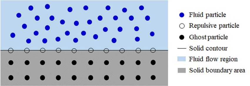
Water 2021, 13, 2276 5 of 13
(a) (b)
Figure 2. Treatment on the interface of different fluids: (a) original particles; (b) converted particles.
2.6.
2.6. Boundary
Boundary Condition
Condition
During
During thethe submarine
submarine debris
debris flow
flow propagation,
propagation, thethe fluid
fluid particles
particles face
face resistance
resistance
from
from the
the local
local seabed.
seabed. Therefore,
Therefore, toto truly
truly simulate
simulate the
thedebris
debrisflow
flowmotion,
motion,ititisisimportant
important
to
to accurately
accurately calculate
calculate the
the repulsive
repulsive force
force from
from the
the solid
solid boundary.
boundary. In In the
the SPH
SPH method,
method,
repulsive
repulsive particles are widely used on the boundary contours to exert a forceon
particles are widely used on the boundary contours to exert a force onthe
thefluid
fluid
particle
particleininthe
thedirection
directionofofthe
theline
lineconnecting
connectingbothbothparticles,
particles,as
asshown
shownin inFigure
Figure3.3.
Figure 3.
Figure 3. Schematic
Schematic illustration
illustration of
of the
the solid
solid boundary
boundary treatment.
treatment.
The
Therepulsive force,FFijij,, can
repulsiveforce, canbe
bedetermined
determinedby
byEquation
Equation(11)
(11)[40]:
[40]:
n1 n2
r0 r Xij r0
− n1 0 ≥1
ij2 ,
D
n2
if
Fij = r0 |−rij| r0 |rX
|rij| ij | , r0|rij | (11)
D if ≥ 1
rij r r0 2
r < 1 r
Fij = 0 i f |rijij|
ij ij
(11)
r0
0
where D is a parameter that depends if on the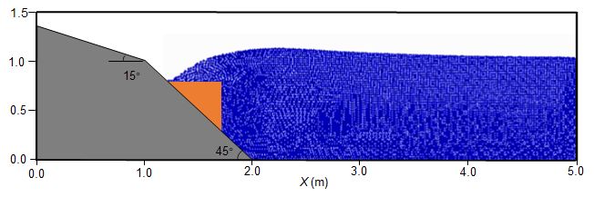
Water 2021, 13, 2276 6 of 13
Figure 4. Experimental setup of an underwater rigid block sliding along an inclined plane.
Table 1. Parameters used in the SPH simulation of the rigid block sliding experiment.
Table 1. Parameters used in the SPH simulation of the rigid block sliding experiment.
Rigid block density ρs (kg/m3) 2000
Rigid block density
Water density ρs (kg/m3 )ρw (kg/m3) 2000
1000
Water density
Water viscosity coefficient ρw (kg/m3 ) η (Pa·s) 1000
1.7 × 10⁻³
Water viscosity coefficient η (Pa·s) 1.7 × 10⁻³
Acceleration of gravity 2 g (m/s2) 9.8
Acceleration of gravity g (m/s ) 9.8
Figure 5 shows the SPH simulated results for the rigid block sliding experiment.
When theFigure 5 shows
block the SPH
slid down, simulated
surge results
waves were for the rigid
generated blockthe
because sliding experiment.
kinetic energy ofWhen
the
the block slid down, surge waves were generated because the kinetic
sliding block was transferred to the ambient water body. The surge waves propagated energy of the sliding
out
block
from thewas
neartransferred
field to thetofar
thefield
ambient water
because body.
of the The surge
height wavesofpropagated
differences out from
the water surface.
the near
Energy field to the
conversion far field
finished because
after of theblock
the rigid height differences
stopped, and of theboth
then waterthe
surface.
kineticEnergy
and
conversion
potential finished
energy of theafter
waterthewaves
rigid block
startedstopped,
to decay.and then
The both theofkinetic
positions andand
the block potential
the
energy of the water waves started to
wave profiles at different times were observed.decay. The positions of the block and the wave profiles
at different times were observed.
(a) t = 0.0 s
Water 2021, 13, x FOR PEER REVIEW 7 of 15
(b) t = 0.5 s
(c) t = 1.0 s
(d) t = 1.5 s
Figure
Figure SPH
5. 5. SPHsimulated
simulatedresults
resultsfor
forthe
therigid
rigidblock
blocksliding experiment: (a) t == 0.0 s; (b) t = 0.5 s; (c) t =
sliding experiment:
= 1.0 s; (d) t == 1.5
1.5 s.
s.
To verify the simulation accuracy of the SPH model, the numerical results were com-
pared with the experimental data from Heinrich [41]. Figure 6 compares the numerical
and experimental vertical displacement time history of the rigid block. The numerical re-
sults coincided with the experiment data well. After an acceleration phase at the begin-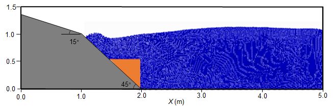
(d) t = 1.5 s
Water 2021, 13, 2276 Figure 5. SPH simulated results for the rigid block sliding experiment: (a) t = 0.0 s; (b) t = 0.5 s; (c)7 of
t 13
= 1.0 s; (d) t = 1.5 s.
To verify the simulation accuracy of the SPH model, the numerical results were com-
paredTo verify
with thethe simulationdata
experimental accuracy
from of the SPH[41].
Heinrich model, the6numerical
Figure compares results were com-
the numerical
pared
and with the experimental
experimental data from Heinrich
vertical displacement time history[41].ofFigure 6 compares
the rigid block. The the numerical
numerical re-and
experimental
sults coincidedvertical
with the displacement
experiment time history
data well. of the
After rigid block. phase
an acceleration The numerical results
at the begin-
coincided
ning, withblock
the rigid the experiment data well.velocity
reached a constant After an ofacceleration phase at the beginning,
0.6 m/s. At approximately 1.0 s, thethe
rigid block reached a constant velocity of 0.6 m/s. At approximately
block reached the flume bottom in the SPH model as well as in the experiment. Figure 1.0 s, the block reached
7
the flume
shows thebottom
comparisonin the between
SPH modeltheassimulated
well as in and
the experiment.
observed wave Figure 7 shows
profiles at the compari-
different
son between
times the
(t = 0.5 s, t =simulated
1.0 s and tand observed
= 1.5 wavesome
s). Although profiles at different
discrepancy cantimes t = 1.0 s
(t = 0.5 s,there
be observed,
and
is t = 1.5
close s). Although
overall agreement some discrepancy
between can be observed,
the experimental there is close
and numerical waveoverall agreement
profiles. The
between the
maximum experimental
run-up and numerical
of the wave during thewave profiles.
simulation wasThe maximum
about 0.10 m,run-up
which of the wave
matches
during
the the simulation
experimental was about 0.10 m, which matches the experimental data well.
data well.
Water 2021, 13, x FOR PEER REVIEW 8 of 15
Comparisonbetween
Figure6.6.Comparison
Figure betweenthe
thenumerical
numericaland
andexperimental
experimentalvertical
verticaldisplacement
displacementtime
timehistory
history of
thethe
of rigid block.
rigid block.
(a) t = 0.5 s
(b) t = 1.0 s
(c) t = 1.5 s
Figure
Figure7. Comparison
7. Comparison between the simulated
between and observed
the simulated wave profiles
and observed at different
wave profiles times: (a)times:
at different t= (a) t =
0.50.5
s; (b) t = t1.0
s; (b) s; (c)s;t(c)
= 1.0 = 1.5
t =s.1.5 s.
To evaluate the performance of the presented model furtherly, the numerical results
are compared with those calculated by Tajnesaie et al. [20] using a MPS model, and Wang
et al. [28] using a coupled DDA-SPH model. Figure 8 compares the water profiles calcu-
lated based on the above-mentioned numerical models at t = 0.5 s and t = 1.0 s. It shows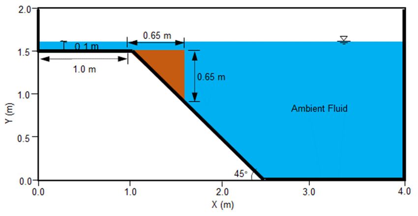
(c) t = 1.5 s
Water 2021, 13, 2276 Figure 7. Comparison between the simulated and observed wave profiles at different times: (a)8 of
t =13
0.5 s; (b) t = 1.0 s; (c) t = 1.5 s.
To evaluate the performance of the presented model furtherly, the numerical results
To evaluate the performance of the presented model furtherly, the numerical results
are compared with those calculated by Tajnesaie et al. [20] using a MPS model, and Wang
are compared with those calculated by Tajnesaie et al. [20] using a MPS model, and Wang
et al. [28] using a coupled DDA-SPH model. Figure 8 compares the water profiles calcu-
et al. [28] using a coupled DDA-SPH model. Figure 8 compares the water profiles calculated
lated based on the above-mentioned numerical models at t = 0.5 s and t = 1.0 s. It shows
based on the above-mentioned numerical models at t = 0.5 s and t = 1.0 s. It shows that
that all the numerical models produce similar water profiles which are consistent with
all the numerical models produce similar water profiles which are consistent with that
that observed in the experiments.
observed in the experiments.
Water 2021, 13, x FOR PEER REVIEW 9 of 15
(a) t = 0.5 s
(b) t = 1.0 s
Figure
Figure8.8.Comparison
Comparisonofof
the
theexperimental
experimental and
andnumerical
numerical (from
(fromthe themodels
modelsofofcurrent
currentstudy
studyand
and
other numerical
other studies)
numerical water
studies) waterprofiles
profilesatatdifferent
differenttimes:
times:(a)(a)t =t =
0.50.5
s; s;
(b) t =t 1.0
(b) s. s.
= 1.0
ToToquantitatively
quantitativelycompare
comparethe theresults,
results,the thePearson
Pearsoncorrelation
correlationcoefficient
coefficient ofofthe
theex-
ex-
perimentaland
perimental andnumerical
numericalwater waterprofilesprofilesininFigure Figure8 8are arecalculated.
calculated.InInthis
thiscase,
case,4040points
points
withananequal
with equalhorizontal
horizontaldistance
distanceonon the
the water
water profile
profile are
are selected
selected asas
thethe analysis
analysis objects.
objects.
Assuming
Assuming that
that thethe vector
vector X (x X1,(x
x21, ,xx3,2……,
, x3 , . x. 40 . . , x40 ) represents
. ). represents the calculated
the calculated elevationselevations
of these
of these
points, points,
and y2, yY
Y (y1, and 3, (y
……,1 , y2y, 40y)3 ,represents
. . . . . . , y40the ) represents
measuredthe measured
ones, ones, correlation
the Pearson the Pearson
correlation coefficient of the two vectors
coefficient of the two vectors can be calculated as: can be calculated as:
nn
(( xii −−xx)()(yyi i−−y )y)
∑
Corr (X,(YX), Y
Corr =) =
s i =i =11
(12)
(12)
nn n n
((xxii − ∑( yi(y−i y−) y)
− xx)) ××
22 2 2
∑
i =i =11 i =1i =1
where xx and
where y the
andy are are average
the average
valuesvalues
of the of two
the two
datadata
sets,sets, respectively.
respectively.
According
AccordingtotoEquation
Equation(12),
(12),the correlation
the correlationcoefficients
coefficientsbetween
betweenthetheexperimental
experimentalandand
numerical
numericalresults
resultsare
arelisted
listed in
in Table
Table 2.2. ItItshows
showsthat
thatall
allthe
thecorrelation
correlation coefficients
coefficients calcu-
calculated
lated are close
are close to 1,towhich
1, which
meansmeansthatthat
thethe numerical
numerical results
results havehave a strong
a strong correlation
correlation with
with the
the experimental profiles. Therefore, the presented SPH model can successfully
experimental profiles. Therefore, the presented SPH model can successfully simulate such simulate
such complex
complex flows.
flows.
Table
Table2.2.
Correlation coefficients
Correlation between
coefficients the experimental
between and numerical
the experimental results
and numerical on theon
results water
the pro-
water
files.
profiles.
Case Case Current Study Tajnesaie
Current Study
et al. [20]
Tajnesaie et al. [20]
Wang et al. [28]
Wang et al. [28]
t = 0.5 0.9336 0.9389 0.9297
t = 0.5 0.9336 0.9389 0.9297
t = 1.0 t = 1.0 0.9132 0.9132 0.9206 0.9206 0.9040
0.9040
3.2. Waves Generated by the Underwater Sand Flow
In Section 3.1, the block was assumed to be rigid, which is not consistent with the
actual situation of submarine debris flow. The large deformation of the solid phase should
be taken into account in the simulation of the submarine debris flow propagation. There-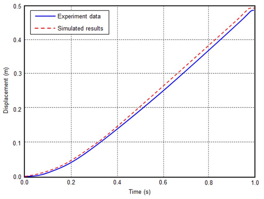
Water 2021, 13, 2276 9 of 13
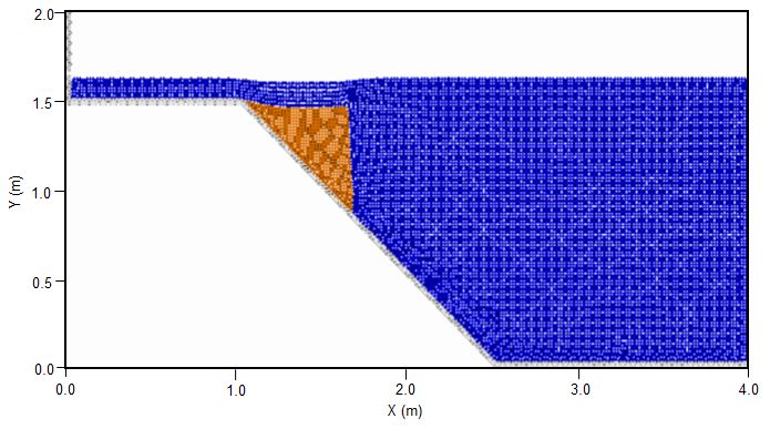
3.2. Waves Generated by the Underwater Sand Flow
In Section 3.1, the block was assumed to be rigid, which is not consistent with the actual
situation of submarine debris flow. The large deformation of the solid phase should be
taken into account in the simulation of the submarine debris flow propagation. Therefore,
an experiment of the surge waves generated by underwater sand flow, conducted by
Rzadkiewicz et al. [42], was simulated. Figure 9 shows the experimental setup. In this
experiment, the maximum water depth was 1.6 m. Under the influence of gravity, a mass
Water 2021, 13, x FOR PEER REVIEW 10 of 15
of sand (0.65 m × 0.65 m in cross section) slid down along a slope of 45◦ , and generated
waves propagated outward.
Figure 9.
Figure Experimentalsetup
9. Experimental setupof
ofthe
theunderwater
underwater sand
sand flow.
flow.
Inthe
theunderwater
underwatersand
sandflow
flowexperiment,
experiment, 3
In thethe density
density of the
of the sandsand
waswas19501950
kg/mkg/m
3, and,
andgrain
the the grain diameter
diameter rangedranged
from 2from 2 to In
to 7 mm. 7 mm. In the numerical
the numerical simulation,simulation, the sand
the sand flow was
flow was assumed to be a Bingham fluid. The parameters are listed in
assumed to be a Bingham fluid. The parameters are listed in Table 3. In the absence Table 3. In the
of
absence of measurements, the viscosity coefficient and yield stress of Bingham model can
measurements, the viscosity coefficient and yield stress of Bingham model can be deter-
be determined by trial and error. According to Ataie–Ashtiani and Shobeyri [43], under
mined by trial and error. According to Ataie–Ashtiani and Shobeyri [43], under the con-
the conditions of viscosity coefficient η = 0.15 Pa·s and Bingham yield stress τ y = 750 Pa,
ditions of viscosity coefficient ηg = 0.15 gPa·s and Bingham yield stress τy = 750 Pa, the nu-
the numerical results match the experimental data well. Therefore, the same parameter
merical results match the experimental data well. Therefore, the same parameter values
values were used in this study.
were used in this study.
Table 3. Parameters used in the SPH simulation of underwater sand flow.
Table 3. Parameters used in the SPH simulation of underwater sand flow.
Density of sandof sand
Density ρs (kg/m3 ) ρs (kg/m3) 1950 1950
Viscosity coefficient of sand flow η g (Pa·s) 0.15
Viscosity coefficient of sand flow ηg (Pa·s) 0.15
Bingham yield stress of sand flow τ y (Pa) 750
Bingham
Densityyield stress of sand flow
of water ρw (kg/m ) τy (Pa)
3 1000 750
Viscosity coefficient ofofwater
Density water η w (Pa·s) ρw (kg/m3) 1.7 × 10−1000
3
Acceleration of gravity
Viscosity coefficient of water g (m/s2 ) ηw (Pa·s) 9.81.7 × 10−3
Acceleration of gravity g (m/s2) 9.8
Figure 10 shows the SPH simulated results for the underwater sand flow. Unlike
Figure 10numerical
the previous shows theexample,
SPH simulated results
the solid phase forno
the underwater
longer behaved sand
as aflow.
rigidUnlike the
block but
previous
deformednumerical example,
significantly whenthe soliddown
sliding phasealong
no longer behaved
the slope. asprofiles
The a rigid block but and
of water de-
formed significantly
sand slope when
at different sliding
times down along
are presented. The the slope.
sand Thekeeps
slope profiles of water
its initial andat
shape sand
the
slope at different times are presented. The sand slope keeps its initial shape
beginning of slide motion, as shown in Figure 9a,b, while at t = 0.8 s, most of the sand at the begin-
ning of slide
particles are motion, as shown
concentrated at theinflow
Figure 9a,b,
front, as while
shownatint = 0.8 s, 9d.
Figure most of the sand particles
are concentrated at the flow front, as shown in Figure 9d.
Figure 11 compares the simulated slope configurations with experimental data [42]
and those calculated by the VOF model proposed in [42] and the ISPH model proposed in
[43]. It shows that the simulated slope configurations are coincident with experimental
results. Table 4 lists the Pearson correlation coefficients of the numerical and experimental
slope configurations shown in Figure 11. The comparison shows that the SPH model pro-
posed in this study has the equivalent simulation accuracy with the existing numerical
models.
Water  2021,13,
 Water2021,  13,2276
                 x FOR PEER REVIEW                                                                                                     11 of 15    10 of 13

                                                                   (a) t = 0.2 s

                                                                   (b) t = 0.4 s

 Water 2021, 13, x FOR PEER REVIEW                                                                                                     12 of 15

                                                                   (c) t = 0.6 s

                                                                   (d) t = 0.8 s
                                 Figure
                                   Figure 10.10.
                                              SPH  simulated
                                                 SPH         results
                                                      simulated      for the
                                                                 results  forunderwater sand flow:
                                                                              the underwater  sand(a) t = 0.2
                                                                                                   flow:   (a)s;t (b) t =s;0.4
                                                                                                                  = 0.2        s; t(c)
                                                                                                                             (b)     = t0.4
                                                                                                                                         = 0.6 s; t = 0.6 s;
                                                                                                                                            s; (c)
                                 (d) t = 0.8 s.
                                   (d) t = 0.8 s.

                                 Table 4. Correlation coefficients between the experimental and numerical results on the water pro-
                                 files.

                                      Case             Current Study                 VOF Results [42]                ISPH Results [43]
                                     t = 0.4              0.9092                         0.8641                           0.9197
(d) t = 0.8 s
Water 2021, 13, 2276 11 of 13
Figure 10. SPH simulated results for the underwater sand flow: (a) t = 0.2 s; (b) t = 0.4 s; (c) t = 0.6 s;
(d) t = 0.8 s.
Table 4.Figure
Correlation coefficients
11 compares thebetween theslope
simulated experimental and numerical
configurations results on the data
with experimental water[42]
pro-and
files.
those calculated by the VOF model proposed in [42] and the ISPH model proposed in [43].
It Case
shows that theCurrent
simulated slope configurations
Study VOF Resultsare coincident
[42] with
ISPHexperimental
Results [43] results.
Table 4
t = 0.4 lists the Pearson correlation
0.9092 coefficients of
0.8641the numerical and experimental
0.9197 slope
configurations shown in Figure 11. The comparison shows that the SPH model proposed in
t = 0.8 0.8761 0.8318 0.8804
this study has the equivalent simulation accuracy with the existing numerical models.
(a) t = 0.4 s
(b) t = 0.8 s
Figure
Figure11.11.Comparison
Comparisonof of
thethe
experimental and
experimental numerical
and numerical(from thethe
(from models
modelsof current study
of current andand
study
other numerical
other numerical studies) slope
studies) configurations
slope at different
configurations times:
at different (a) (a)
times: t = t0.4 s; (b)
= 0.4 t = 0.8
s; (b) t = s.
0.8 s.
Table 4. Correlation coefficients between the experimental and numerical results on the water profiles.
Case Current Study VOF Results [42] ISPH Results [43]
t = 0.4 0.9092 0.8641 0.9197
t = 0.8 0.8761 0.8318 0.8804
4. Conclusions
Submarine debris flow-generated water waves are natural phenomena that occur
under certain conditions and can result in damage of infrastructure and loss of life in
coastal areas. In this study, an SPH model with a multiphase granular flow algorithm
is presented for numerical simulation of surge waves generated by submarine debris
flows. The Bingham fluid model and Newton fluid model are used to describe the motion
behavior of submarine debris flow and ambient water, respectively. A simple treatment is
proposed to ensure the continuity of the density and pressure near the interface of these
two fluids and to avoid numerical instability.
This model was first used to simulate an experiment of underwater rigid block sliding.
The simulated wave profiles were compared with the observed results to verify the stability
and accuracy of the SPH model.Water 2021, 13, 2276 12 of 13
Then, this model was applied to simulate submarine debris flow. Surged waves
generated by the underwater sand flow were computed and compared with the tested
results. The good agreement between the numerical and tested results proves that the
proposed SPH model is suitable to simulate such complex flows.
In fact, submarine debris flows move across 3D submarine topography and may
change direction and split or join in response to the complex topography. Therefore, the 2D
model presented in this study cannot truly reproduce the complex dynamic process, and
a 3D model with parallel computing techniques is necessary to improve the calculation
accuracy and efficiency.
Author Contributions: Conceptualization, Z.D. and S.Q.; methodology, Z.D. and J.X.; writing—
original draft preparation, Z.D. and J.X.; writing—review and editing, S.Q. and S.C.; visualization,
J.X. and S.C.; supervision, S.Q.; funding acquisition, Z.D. All authors have read and agreed to the
published version of the manuscript.
Funding: This research was funded by the National Natural Science Foundation of China (grant
No. 42102318) and the Program for Professor of Special Appointment (Eastern Scholar) at Shanghai
Institutions of Higher Learning.
Institutional Review Board Statement: Not applicable.
Informed Consent Statement: Not applicable.
Data Availability Statement: The data presented in this study are available on request from the
corresponding author.
Acknowledgments: The authors are grateful for the support from the Department of Civil Engineer-
ing, Shanghai University.
Conflicts of Interest: The authors declare no conflict of interest.
References
1. Nian, T.K.; Guo, X.S.; Zheng, D.F.; Xiu, Z.X.; Jiang, Z.B. Susceptibility assessment of regional submarine landslides triggered by
seismic actions. Appl. Ocean Res. 2019, 93, 101964. [CrossRef]
2. Gonzalez-Vida, J.M.; Macias, J.; Castro, M.J.; Sanchez-Linares, C.; de la Asuncion, M.; Ortega-Acosta, S.; Arcas, D. The Lituya Bay
landslide-generated mega-tsunami—numerical simulation and sensitivity analysis. Nat. Hazards Earth Syst. Sci. 2019, 19, 369–388.
[CrossRef]
3. Dan, G.; Sultan, N.; Savoye, B. The 1979 Nice harbour catastrophe revisited: Trigger mechanism inferred from geotechnical
measurements and numerical modelling. Mar. Geol. 2007, 245, 40–64. [CrossRef]
4. Rabinovich, A.B.; Thomson, R.E.; Kulikov, E.A.; Bornhold, B.D.; Fine, I.V. The landslide-generated tsunami of November 3, 1994
in Skagway Harbor, Alaska: A case study. Geophys. Res. Lett. 1999, 26, 3009–3012. [CrossRef]
5. Sabeti, R.; Heidarzadeh, M. Semi-empirical predictive equations for the initial amplitude of submarine landslide-generated
waves: Applications to 1994 Skagway and 1998 Papua New Guinea tsunamis. Nat. Hazards 2020, 103, 1591–1611. [CrossRef]
6. Heidarzadeh, M.; Satake, K. Source properties of the 17 July 1998 Papua New Guinea tsunami based on tide gauge records.
Geophys. J. Int. 2015, 202, 361–369. [CrossRef]
7. Hébert, H.; Burg, P.E.; Binet, R.; Lavigne, F.; Allgeyer, S.; Schindelé, F. The 2006 July 17 Java (Indonesia) tsunami from satellite
imagery and numerical modelling: A single or complex source? Geophys. J. Int. 2012, 191, 1255–1271. [CrossRef]
8. Poupardin, A.; Calais, E.; Heinrich, P.; Hebert, H.; Rodriguez, M.; Leroy, S.; Aochi, H.; Douilly, R. Deep submarine landslide
contribution to the 2010 Haiti earthquake tsunami. Nat. Hazards Earth Syst. Sci. 2020, 20, 2055–2065. [CrossRef]
9. Muhari, A.; Imamura, F.; Arikawa, T.; Hakim, A.; Afriyanto, B. Solving the Puzzle of the September 2018 Palu, Indonesia, Tsunami
Mystery: Clues from the Tsunami Waveform and the Initial Field Survey Data. J. Disaster Res. 2018, 13, sc20181108. [CrossRef]
10. Arikawa, T.; Muhari, A.; Okumura, Y.; Dohi, Y.; Afriyanto, B.; Sujatmiko, K.A.; Imamura, F. Coastal subsidence induced several
tsunamis during the 2018 Sulawesi earthquake. J. Disaster Res. 2018, 13, sc20181204. [CrossRef]
11. Sassa, S.; Takagawa, T. Liquefied gravity flow-induced tsunami: First evidence and comparison from the 2018 Indonesia Sulawesi
earthquake and tsunami disasters. Landslides 2019, 16, 195–200. [CrossRef]
12. Mohammed, F.; Fritz, H.M. Physical modeling of tsunamis generated by three-dimensional deformable granular landslides. J.
Geophys. Res. Ocean 2012, 117, C11015. [CrossRef]
13. McFall, B.C.; Fritz, H.M. Physical modelling of tsunamis generated by three-dimensional deformable granular landslides on
planar and conical island slopes. Proc. R. Soci. A Math. Phys. Eng. Sci. 2016, 472, 20160052. [CrossRef] [PubMed]
14. Wang, Y.; Liu, J.Z.X.; Li, D.Y.; Yan, S.J. Optimization model for maximum tsunami amplitude generated by riverfront landslides
based on laboratory investigations. Ocean Eng. 2017, 142, 433–440. [CrossRef]Water 2021, 13, 2276 13 of 13
15. Miller, G.S.; Take, W.A.; Mulligan, R.P.; McDougall, S. Tsunamis generated by long and thin granular landslides in a large flume.
J. Geophys. Res. Ocean 2017, 122, 653–668. [CrossRef]
16. Meng, Z.Z. Experimental study on impulse waves generated by a viscoplastic material at laboratory scale. Landslides 2018, 15,
1173–1182. [CrossRef]
17. Takabatake, T.; Mall, M.; Han, D.C.; Inagaki, N.; Kisizaki, D.; Esteban, M.; Shibayama, T. Physical modeling of tsunamis generated
by subaerial, partially submerged, and submarine landslides. Coast. Eng. J. 2020, 4, 582–601. [CrossRef]
18. Lynett, P.; Liu, P.L.F. A numerical study of submarine-landslide-generated waves and run-up. Proc. R. Soc. A Math. Phys. Eng. Sci.
2002, 458, 2885–2910. [CrossRef]
19. Yavari-Ramshe, S.; Ataie-Ashtiani, B. Numerical modeling of subaerial and sub- marine landslide-generated tsunami waves-recent
advances and future challenges. Landslides 2016, 13, 1325–1368. [CrossRef]
20. Tajnesaie, M.; Shakibaeinia, A.; Hosseini, K. Meshfree particle numerical modelling of sub-aerial and submerged landslides.
Comput. Fluids 2018, 172, 109–121. [CrossRef]
21. Sun, J.K.; Wang, Y.; Huang, C.; Wang, W.H.; Wang, H.B.; Zhao, E.J. Numerical investigation on generation and propagation
characteristics of offshore tsunami wave under landslide. Appl. Sci. 2020, 10, 5579. [CrossRef]
22. Rupali; Kumar, P.; Rajni. Spectral wave modeling of tsunami waves in Pohang New Harbor (South Korea) and Paradip Port
(India). Ocean Dyn. 2020, 70, 1515–1530. [CrossRef]
23. Baba, T.; Gon, Y.; Imai, K.; Yamashita, K.; Matsuno, T.; Hayashi, M.; Ichihara, H. Modeling of a dispersive tsunami caused by a
submarine landslide based on detailed bathymetry of the continental slope in the Nankai trough, southwest Japan. Tectonophysics
2019, 768, 228182. [CrossRef]
24. Yao, Y.; He, T.; Deng, Z.; Chen, L.; Guo, H. Large eddy simulation modeling of tsunami-like solitary wave processes over fringing
reefs. Nat. Hazards Earth Syst. Sci. 2019, 19, 1281–1295. [CrossRef]
25. Zhao, E.; Sun, J.; Tang, Y.; Mu, L.; Jiang, H. Numerical investigation of tsunami wave impacts on different coastal bridge decks
using immersed boundary method. Ocean Eng. 2020, 201, 107132. [CrossRef]
26. Lucy, L.B. A numerical approach to the testing of the fission hypothesis. Astrophys. J. 1977, 82, 1013–1024. [CrossRef]
27. Iryanto, I. SPH simulation of surge waves generated by aerial and submarine landslides. J. Phys. Conf. Ser. 2019, 1245, 012062. [CrossRef]
28. Wang, W.; Chen, G.Q.; Zhang, H.; Zhou, S.H.; Liu, S.G.; Wu, Y.Q.; Fan, F.S. Analysis of landslide-generated impulsive waves
using a coupled DDA-SPH method. Eng. Anal. Bound. Elem. 2016, 64, 267–277. [CrossRef]
29. Gingold, R.A.; Monaghan, J.J. Smoothed particle hydrodynamics: Theory and application to non-spherial stars. Mon. Not. R.
Astron. Soc. 1977, 181, 375–389. [CrossRef]
30. Dai, Z.L.; Huang, Y.; Cheng, H.L.; Xu, Q. SPH model for fluid–structure interaction and its application to debris flow impact
estimation. Landslides 2017, 14, 917–928. [CrossRef]
31. Dai, Z.L.; Huang, Y.; Xu, Q. A hydraulic soil erosion model based on a weakly compressible smoothed particle hydrodynamics
method. Bull. Eng. Geol. Environ. 2019, 78, 5853–5864. [CrossRef]
32. Jamalabadi, M.Y.A. Frequency analysis and control of sloshing coupled by elastic walls and foundation with smoothed particle
hydrodynamics method. J. Sound Vib. 2020, 476, 115310. [CrossRef]
33. Price, D.J.; Laibe, G. A solution to the overdamping problem when simulating dust-gas mixtures with smoothed particle
hydrodynamics. Mon. Not. R. Astron. Soc. 2020, 495, 3929–3934. [CrossRef]
34. Ma, C.; Iijima, K.; Oka, M. Nonlinear waves in a floating thin elastic plate, predicted by a coupled SPH and FEM simulation and
by an analytical solution. Ocean Eng. 2020, 204, 107243. [CrossRef]
35. Liu, M.B.; Liu, G.R. Smoothed particle hydrodynamics (SPH): An overview and recent developments. Arch. Comput. Methods Eng.
2010, 17, 25–76. [CrossRef]
36. Shakibaeinia, A.; Jin, Y.C. MPS mesh-free particle method for multiphase flows. Comput. Methods Appl. Mech. Eng. 2012, 229,
13–26. [CrossRef]
37. Monaghan, J.J.; Cas, R.F.; Kos, A.; Hallworth, M. Gravity currents descending a ramp in a stratified tank. J. Fluid Mech. 1999, 379,
39–70. [CrossRef]
38. Zheng, B.; Chen, Z. A multiphase smoothed particle hydrodynamics model with lower numerical diffusion. J. Comput. Phys.
2019, 382, 177–201. [CrossRef]
39. Zhang, W.J.; Ji, J.; Gao, Y.F. SPH-based analysis of the post-failure flow behavior for soft and hard interbedded earth slope. Eng.
Geol. 2020, 267, 105446. [CrossRef]
40. Monaghan, J.J. Simulating free surface flows with SPH. J. Comput. Phys. 1994, 110, 399–406. [CrossRef]
41. Heinrich, P. Nonlinear water waves generated by submarine and aerial landslides. J. Waterw. Port Coast. Ocean Eng. 1992, 118,
249–266. [CrossRef]
42. Rzadkiewicz, S.A.; Mariotti, C.; Heinrich, P. Numerical simulation of submarine landslides and their hydraulic effects. J. Waterw.
Port Coast. Ocean Eng. 1997, 123, 149–157. [CrossRef]
43. Ataie-Ashtiani, B.; Shobeyri, G. Numerical simulation of landslide impulsive waves by incompressible smoothed particle
hydrodynamics. Int. J. Numer. Methods Fluids 2008, 56, 209–232. [CrossRef]You can also read