Reconstruction of Solid Models from Oriented Point Sets
←
→
Page content transcription
If your browser does not render page correctly, please read the page content below
Eurographics Symposium on Geometry Processing (2005)
M. Desbrun, H. Pottmann (Editors)

      Reconstruction of Solid Models from Oriented Point Sets

                                                        Michael Kazhdan†

        Abstract
        In this paper we present a novel approach to the surface reconstruction problem that takes as its input an oriented
        point set and returns a solid, water-tight model. The idea of our approach is to use Stokes’ Theorem to compute
        the characteristic function of the solid model (the function that is equal to one inside the model and zero outside
        of it). Specifically, we provide an efficient method for computing the Fourier coefficients of the characteristic
        function using only the surface samples and normals, we compute the inverse Fourier transform to get back the
        characteristic function, and we use iso-surfacing techniques to extract the boundary of the solid model.
        The advantage of our approach is that it provides an automatic, simple, and efficient method for computing the
        solid model represented by a point set without requiring the establishment of adjacency relations between samples
        or iteratively solving large systems of linear equations. Furthermore, our approach can be directly applied to
        models with holes and cracks, providing a method for hole-filling and zippering of disconnected polygonal models.
        Categories and Subject Descriptors (according to ACM CCS): I.3.5 [Computer Graphics]: Computational Geometry
        and Object Modeling

1. Introduction                                                     gration filter. (3) The reconstructed surface is extracted as an
                                                                    iso-surface of the voxel grid.
Reconstructing 3D surfaces from point samples is a well
studied problem in computer graphics. The ability to recon-            The advantage of our approach is its simplicity: Splat-
struct such surfaces provides a method for zippering sam-           ting the oriented point samples into the voxel grid can be
ples obtained through scanning, filling in holes in models          done without necessitating the establishment of adjacency
with degeneracies, and re-meshing existing models. While            relations between the samples. Convolving with a filter
there has been much work in this area, we provide a novel           can be efficiently performed using the Fast Fourier Trans-
approach that is based on basic calculus, providing a simple        form [FFTW]. And finally, standard methods such as the
method for reconstructing solid models from oriented point          Marching Cubes algorithm [LC87] can be used to extract the
sets (point samples with associated normals).                       reconstructed surface, returning a triangulation that is guar-
                                                                    anteed to be water-tight.
   Our approach takes advantage of the fact that an oriented
point set sampled from the surface of a solid model provides           Figure 1 demonstrates our method for an oriented point
precisely enough information for computing surface inte-            set obtained by sampling the surface of a dinosaur head. The
grals. Thus, by formulating the solution of the surface recon-      original model is shown on the left, the samples are shown
struction problem in terms of volume integrals, we can apply        in the middle, and the reconstructed model is shown on the
Stokes’ Theorem to transform the volume integrals into sur-         right. Note that even though the points were sampled from
face integrals and compute a discrete approximation using           a model which was not water-tight, (there are holes in the
the oriented point samples.                                         eyes, the nostrils, and the mouth) our method succeeds in re-
   In practice, our approach provides a method for recon-           turning a seamless mesh that closely approximates the input
structing a water-tight model from an oriented point set in         data, accurately capturing the fine model details.
three easy steps: (1) The point-normal pairs are splatted into         Our method addresses the surface reconstruction problem
a voxel grid. (2) The voxel grid is convolved with an inte-         by approximating integration by a discrete summation and a
                                                                    direct implementation of our method assumes that the sam-
                                                                    ples are uniformly distributed over the surface of a model.
† Johns Hopkins University                                          However, in many situations, the input samples are not uni-

c The Eurographics Association 2005.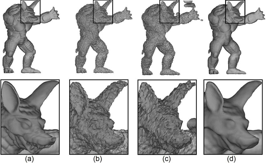
M. Kazhdan / Reconstruction of Solid Models

                                                                         inefficient for large point samples. Second, these methods
                                                                         tend to perform less effectively when the point samples are
                                                                         not uniformly distributed over the surface of the model.
                                                                            Surface fitting methods approach the reconstruction prob-
                                                                         lem by deforming a base model to optimally fit the input
Figure 1: The initial model (left), a non-uniform sampling of points     sample points [TV91, CM95]. These approaches represent
from the model (middle), and the reconstructed water-tight, surface      the base shape as a collection of points with springs between
obtained using our method (right).                                       them and adapt the shape by adjusting either the spring stiff-
                                                                         nesses or the point positions as a function of the surface in-
formly distributed. To this end, we also present a simple
                                                                         formation. As with the computational geometric approaches,
heuristic method that assigns a weight to each point-normal
                                                                         these methods have the advantage of generating a surface re-
pair corresponding to the sampling density about the sample.
                                                                         construction whose complexity is on the order of the size of
We show that this heuristic provides a robust method for as-
                                                                         the input samples. However, these methods tend to be re-
signing weights that approximate the regional sampling den-
                                                                         strictive as the topology of the reconstructed surface needs
sity allowing for the reconstruction of surfaces from samples
                                                                         to be the same as the topology of the base shape, limiting the
that are not uniformly distributed. Figure 1 shows an exam-
                                                                         class of models that can be reconstructed using this method.
ple of the use of this method: Though, the samples are not
uniformly distributed over the surface of the original triangu-             The third class of approaches taken in reconstruct-
lation, with denser sampling in regions of higher curvature,             ing surfaces uses the point samples to define an
our weighting method assigns the correct weights to the sam-             implicit function in 3D and then extracts the re-
ples and the reconstructed surface closely approximates the              constructed surface as an iso-surface of the function,
input sample in regions of both dense and sparse sampling.               [HD∗ 92, CL96, Wh98, CB∗ 01, DM∗ 02, OBS04, TO04].
   The remainder of this paper is structured as follows: In              The advantage of these types of approaches is two-fold:
Section 2 we review previous work in surface reconstruction.             First, the extracted surface is always guaranteed to be
We present our approach in Section 3 and provide results and             water-tight, returning a model with a well-defined interior
discussion in Section 4. Finally, we conclude in Section 5 by            and exterior, and second, the use of an implicit function does
summarizing our results and discussing possible directions               not place any restrictions on the topological complexity
for future research.                                                     of the extracted iso-surface, providing a reconstruction
                                                                         algorithm that can be applied to many different 3D models.
                                                                         In general, this type of approach has the limitation that
2. Related Work                                                          the complexity of the reconstruction process is a function
The importance of the surface reconstruction problem has                 of the resolution of the voxel grid, not the output surface,
motivated a large body of research in computer graphics                  and many of these approaches use hierarchical structures
and previous approaches can be broadly grouped into one of               to localize the definition of the implicit function to a thin
three categories: (1) Methods that address the surface recon-            region about the input samples, thereby reducing both the
struction problem through the use of computational geome-                storage and computational complexity of the reconstruction.
try techniques, (2) methods that address the surface recon-
struction problem by directly fitting a surface to the point             3. Approach
samples, and (3) methods that address the surface recon-
struction problem by fitting a 3D function to the point sam-             The goal of our work is to provide a method that takes as
ples and then extracting the reconstructed surface as an iso-            its input an oriented point set sampled from the surface of a
surface of the implicit function.                                        model and returns a water-tight reconstruction of the surface.
                                                                         Our approach is to construct the characteristic function of
   In general, the computational geometry based meth-
                                                                         the solid defined by the point samples – the function whose
ods proceed by computing either the Delaunay trian-
                                                                         value is one inside of the solid and zero outside of it – and
gulation of the point samples or the dual Voronoi di-
                                                                         then to extract the appropriate iso-surface.
agram and using the cells of these structures to de-
fine the topological connectivity between the point sam-                    To compute the characteristic function of the solid we
ples [Bo84, EM94, ABK98, AC∗ 00, ACK01, DG03]. The                       compute its Fourier coefficients. In practice, one would com-
advantage of these types of approaches is that the complexity            pute the Fourier coefficients by integrating the complex
of the reconstructed surface is on the order of the complex-             exponentials over the interior of the model. However, by
ity of the input samples. Moreover, for many of these recon-             Stokes’ Theorem, we can express this volume integral as a
struction methods, it is possible to bound the quality of the            surface integral, only using information about the positions
reconstruction if the sampling density is known. However,                and the normals of points on the boundary. Since this is pre-
these methods suffer from two limitations: First, they require           cisely the information provided as the input to our method
the computation of the Delaunay triangulation which can be               we have sufficient information to compute the Fourier coef-

                                                                                                            c The Eurographics Association 2005.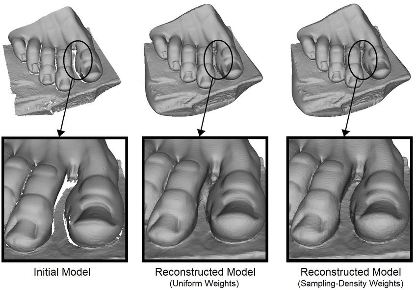
M. Kazhdan / Reconstruction of Solid Models
ficients of the characteristic function, allowing us to use the Our goal is to compute the characteristic function by com-
inverse Fourier transform to compute its values. puting its Fourier coefficients. Specifically, if M is a solid
model and χM is its characteristic function, we would like to
We begin our discussion by reviewing Stokes’ theorem.
compute the coefficients:
Next, we provide a method for expressing each of the Fourier
coefficients of the characteristic function in terms of a sur-
Z
χ̂M (l, m, n) = χM (x, y, z)e−i(lx+my+nz) dxdydz
face integral. Then, we provide an efficient method for com- ZR
3
puting the Fourier coefficients and describe a method for se- = e−i(l px +mpy +npz ) d p.
lecting the iso-value to be used for the iso-surface extrac- p∈M
tion. Finally, we provide a simple heuristic for addressing
(Note that since the function χM is equal to one inside
the problem of non-uniformly sampled input data.
the model and zero outside, integrating the complex ex-
ponentials against the characteristic function is equivalent
3.1. Stokes’ Theorem to computing the integral of these functions over the solid
model.) Using the Divergence Theorem, we know that if
Stokes’ Theorem is an extension of the Fundamental The- ~Fl,m,n : R3 → R3 is a function such that:
orem of Calculus which provides a method for expressing
the integral of a function over the interior of a region as an ∇ · ~Fl,m,n (x, y, z) = e−i(lx+my+nz)
integral over the region’s boundary. In our work, we will be
considering a specific instance of Stokes’ Theorem known as the volume integral can be expressed as the surface integral:
the Divergence Theorem or Gauss’s Theorem. Specifically, Z Z
if M ⊂ R3 is a three-dimensional solid and ~F = (Fx , Fy , Fz ) : χ̂M (l, m, n) = e−i(l px +mpy +npz ) d p = h~F(p),~n(p)id p
M ∂M
R3 → R3 is a vector-valued function, the Divergence Theo-
rem expresses the volume integral as a surface integral: where ~n(p) is the unit normal of the surface ∂ M at p.
Since the input to our algorithm is an oriented point set,
Z Z
∇ · ~F(p)d p = h~F(p),~n(p)id p we can compute the Fourier coefficients of the character-
M ∂M
istic function using a Monte-Carlo approximation. Specifi-
where ∇ · ~F = ∂ Fx /∂ x + ∂ Fy /∂ y + ∂ Fz /∂ z is the divergence cally, given the points {~p1 , . . . ,~pN } with associated normals
of ~F and ~n(p) is the surface normal at the point p. {~n1 , . . . ,~nN }, we set:
Our approach is motivated by the observation that if 1 N
{~pi ,~ni } ⊂ M is a uniformly sampled point set, the volume χ̂M (l, m, n) =
N ∑ h~Fl,m,n (~p j ),~n j i.
integral can be approximated using Monte-Carlo integration: j=1
|M| N ~ In order to be able to evaluate the above summation ex-
Z
M
∇ · ~F(p)d p ≈ ∑ hF(~pi ),~ni i.
N i=1 plicitly, we need to choose the functions ~Fl,m,n whose diver-
gences are equal to the complex exponentials. Perhaps the
In the next section, we show that the surface reconstruction
most direct way to do this is to set ~Fl,m,n to be the function:
problem can be reduced to the computation of volume inte-
grals. Using the above Monte-Carlo approximation, we can i
−i(lx+my+nz)
l+m+n e
compute these volume integrals as a summation over a set ~Fl,m,n (x, y, z) = i
e−i(lx+my+nz) .
l+m+n
of surface samples, providing a method for reconstructing i −i(lx+my+nz)
surfaces from oriented point sets. l+m+n e
The limitation of this type of function is that it is anisotropic,
treating different directions differently. Thus, the obtained
3.2. Defining the Fourier Coefficients characteristic function does not rotate with the model.
To reconstruct a surface from a set of samples, we will first To avoid this problem, we use functions ~Fl,m,n that do not
construct the characteristic function of the solid model. This depend on the alignment of the coordinate axis:
is a function defined in 3D whose value is equal to one inside
the solid and zero outside. Once the characteristic function il
e−i(lx+my+nz)
l 2 +m2 +n2
is obtained, we can obtain the surface by using iso-surface l 2 +mim2 +n2 e−i(lx+my+nz) .
~Fl,m,n (x, y, z) =
(1)
extraction. Instead of computing the characteristic function in
e −i(lx+my+nz)
directly, we first compute its Fourier coefficients and then l 2 +m2 +n2
compute the inverse Fourier Transform of these coefficients. Figure 2 demonstrates the differences in the characteristic
Though less direct, this approach is easy to implement be- function obtained using the different ~Fl,m,n for individual
cause the Fourier coefficients can be expressed as volume point samples with different normal orientations (left and
integrals and hence can be computed from an oriented point middle) and a point set consisting of 100 points randomly
set with a Monte-Carlo approximation of Stokes’ Theorem. distributed over the boundary of the square. The middle row
c The Eurographics Association 2005.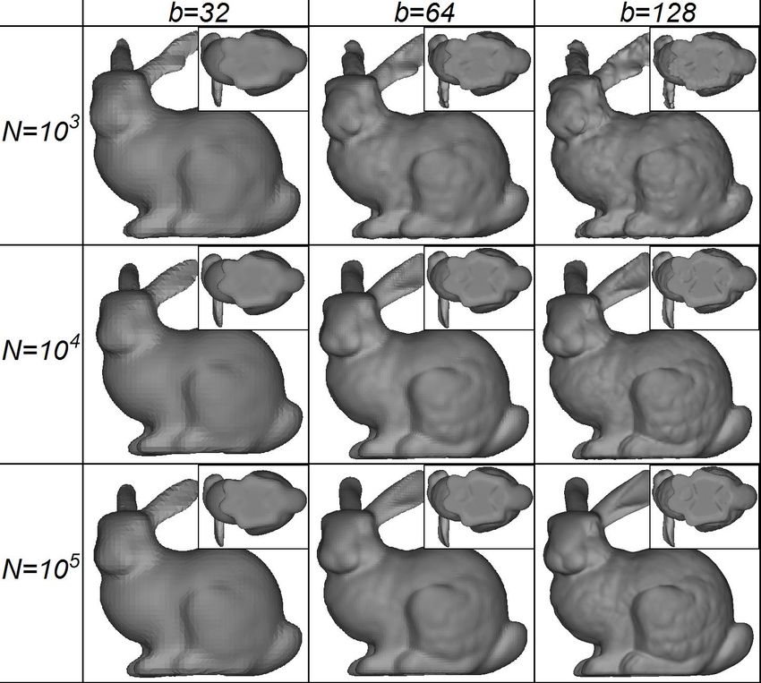
M. Kazhdan / Reconstruction of Solid Models

                                                                         struction we obtain a reconstruction algorithm with com-
                                                                         plexity O(b3 log b + N), (as compared to the O(b3 N) com-
                                                                         plexity of the explicit summation approach).
                                                                           Our approach is to represent the oriented point set by a
                                                                         gradient field which is almost everywhere zero except at the
                                                                         sample locations. At these locations the value of the gradi-
                                                                         ent field is equal to the normal of the corresponding point
                                                                         sample. Specifically, we set ~N : R3 → R3 to be the function:
                                                                                                                 N
                                                                                                ~N(~p) = 1       ∑ δ~p (~p)~n j
                                                                                                         N      j=1
                                                                                                                          j

                                                                         where δ~p is the Kronecker Delta function centered at ~p. The
                                                                         advantage of this representation is that its Fourier coeffi-
                                                                         cients are closely related to the Fourier coefficients of the
Figure 2: Characteristic functions obtained from a point with a          characteristic function. Specifically, if we set ~l = (l, m, n)
90◦ degree normal (left), a point with a 60◦ degree normal (middle),     then the ~l-th Fourier coefficients of the characteristic func-
and a point set sampled from the boundary of a square (right). Re-       tion and the ~l-th Fourier coefficients of the gradient field are:
constructions are shown using the functions ~Fl,m,n whose coordinate
                                                                                              N                                            N
functions are equal (middle) and functions defined by Equation 1                        i                                      ˆ ~l) = 1
                                                                                              ∑ e−ihl,~p i h~n j ,~li                      ∑ e−ihl,~p i~n j .
                                                                                                        ~                                          ~
                                                                         χ̂M (~l) =                         j                 ~N(                      j
(bottom). Points with positive value are drawn in white, points with                  Nklk2
                                                                                        ~                                              N
                                                                                              j=1                                          j=1
negative value in black, and points with zero-value in gray.
                                                                         Thus, the ~l-th Fourier coefficient of the characteristic func-
shows the characteristic function obtained using the func-               tion can be obtained by multiplying the ~l-th Fourier coeffi-
tions ~Fl,m,n whose coordinate functions are equal. In this              cient of the gradient field by i/k~lk2 and taking the dot prod-
case, the anisotropic nature of the function results in charac-          uct with the vector ~l:
teristic functions that do not rotate with the normals, result-
                                                                                                          i ~ˆ ~ ~
ing in a non-uniform distribution of noise in the reconstruc-                               χ̂M (~l) =       hN(l), li.
tion of the square. In contrast, the characteristic functions                                          k~lk2
obtained using Equation 1 (botom) rotate with the normals                                                   ˆ ~l) is a 3D complex vec-
                                                                         (Note that, by abuse of notation, ~N(
and give rise to a smoother reconstruction. (The uniqueness
                                                                         tor, obtained by computing the Fourier coefficients of each
of the functions ~Fl,m,n is discussed in the Appendix.)
                                                                         of the coordinate functions of ~N independently.)
   One should note that computing the Fourier Coefficient of
                                                                            In practice, we implement this reconstruction of the char-
the characteristic function using a Monte-Carlo approxima-
                                                                         acteristic function by “splatting” the sample normals into a
tion of Stokes’ Theorem defines all the Fourier coefficients
                                                                         voxel grid, (where each voxel stores a 3-vector) and then
of the characteristic function except the constant order term.
                                                                         convolving the “splatting” function with a filter ~F whose
Thus, the obtained function is well defined up to an additive
                                                                         (l, m, n)-th Fourier coefficient is:
constant. Furthermore, in the case that we do not know the
sampling density (i.e. the surface area associated with each                                   ˆ m, n) =
                                                                                              ~F(l,                 i(l, m, n)
                                                                                                                                 .
sample point), the resultant characteristic function is only                                                    (l 2 + m2 + n2 )
well defined up to a multiplicative constant.
                                                                         This is an extended notion of the standard convolution. In
                                                                         general, convolving the point samples with a filter results in
3.3. Computing the Fourier Coefficients                                  a function that is the sum of the filters centered at each of
                                                                         the sample points. The result of our extended convolution is
While the method described in the previous section provides              a summation of filters that are not only centered at the sam-
a direct way for obtaining the Fourier coefficients of the               ple points but also aligned with the normals. Intuitively, this
characteristic function, it requires a summation over all of             means that the reconstruction of the characteristic function
the input samples to compute a single Fourier coefficient.               is performed by taking functions shown in the bottom row
Thus, in the case that both the number of input samples                  of Figure 2, translating them to align with the sample points
and the reconstruction band-width are large, explicitly com-             and rotating them to align with the normals.
puting the summation becomes prohibitively slow. In this
section, we show that this summation can be expressed as                   One can view this reconstruction of the characteristic
a convolution so that the Fast Fourier Transform can be                  function as an integration. Specifically, we know that inte-
used to compute the characteristic function efficiently. Con-            gration acts on the complex exponentials by:
sequently, if N is the number of input samples and b is the                                         Z
                                                                                                                      −i ikθ
reconstruction band-width, using the FFT for surface recon-                                             eikθ d θ =      e
                                                                                                                      k

                                                                                                                        c The Eurographics Association 2005.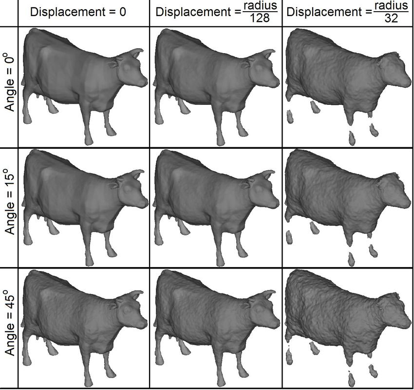
M. Kazhdan / Reconstruction of Solid Models

so that integration is equivalent to convolution with a filter             In the case that the sampling density about each point is
whose k-th Fourier coefficient is −ik/kkk2 . In this context,           given, we can address the problem of non-uniformity in the
multiplication of the ~l-th Fourier coefficient of ~N by i~l/k~lk2      standard manner – weighing the contribution of each sam-
can be viewed as an integration of the surface gradient field           ple point to the overall integral as a function of the sampling
– a vector field which points in the direction of the surface           density. Specifically, we assign a weight to each sample that
normals at the surface points and is zero everywhere else.              is the reciprocal of the regional sampling density and pro-
Integrating this gradient field, we obtain a function that is           ceed as before: (1) We scale each normal by the weight of
constant almost everywhere, with a sharp change in value at             its sample and splat the weighted normals into a voxel grid,
the sample points so that points interior to the model all have         (2) we convolve the voxel grid with the integration filter, and
the same constant value ci and points outside all have the              (3) we extract the iso-surface at the iso-value equal to the
same constant value co , with co 6= ci . (We make the normals           weighted average of the iso-function at the sample locations.
inward facing so that the value of the characteristic function
                                                                          For the case that we do not know the sampling density a
is larger inside the model and smaller outside. This gives rise
                                                                       priori, we propose a simple heuristic for assigning weights to
to the change in sign of the integration filter.)
                                                                       the samples. Our approach is based on the observation that
                                                                       the 3D function obtained by summing Gaussians centered
3.4. Extracting the Iso-Surface                                        at each of the sample points has the property that the value
                                                                       of the function is proportional to the local sampling density.
In order to extract an iso-surface from the characteristic             This motivates the following approach for assigning weights
function, we need to choose an appropriate iso-value. We               to the samples: We “splat” the samples into a voxel grid –
describe two ways in which this can be done.                           adding a value of one to each voxel whose position corre-
                                                                       sponds to the position of a sample – and convolve with a
   First, we can use the fact that the characteristic function
                                                                       Gaussian filter. We then assign a weight to each sample point
has a value of one inside the solid and a value of zero out-
                                                                       ~p which is the reciprocal of the value of the convolution at ~p.
side of it. This motivates choosing an iso-value equal to 0.5.
                                                                       Since the value of the convolution at a point is proportional
Since, as discussed in the previous section, the characteristic
                                                                       to the local sampling density, the reciprocal is proportional
function is only defined up to an additive constant, we would
                                                                       to the surface area associated to the point, providing the ap-
first need to compute the constant order coefficient, or solid
                                                                       propriate weighting for the Monte-Carlo integration.
volume. (This can be done, for example, by using a func-
                                (x,y,z)
tion such as ~F0,0,0 (x, y, z) = 3 .) However, this type of                While this method is easy to implement and we find that
approach has two limitations: First, it assumes that the sam-           it works well in practice, we stress that it is only a heuristic
pling density is given so that the ambiguity in the multiplica-         as it assigns a weight that is inversely proportional to the 3D
tive scale factor of the characteristic function has been re-           sampling density, not the sampling density over the surface.
solved. Second, and more important, this method fails to be
robust in the case when the input points are samples from a
                                                                        4. Results and Discussion
model that is not water-tight. In this case, the computed vol-
ume will vary with the translational alignment of the points            In order to determine how well our method works in practice,
and the shape of the reconstructed surface will depend on the           we ran our reconstruction approach on oriented point sets
coordinate frame of input samples.                                      obtained by sampling triangulated models and compared the
                                                                        obtained reconstruction with the initial model. Specifically,
   Instead, we can compute the average value of the obtained            we designed our experiments to evaluate the quality of the
characteristic function at the sample positions ~p j . Since we         reconstruction as a function of the number of samples, the
would like the input points to lie on the reconstructed sur-            band-width of the reconstruction, the presence of holes and
face, we simply set the iso-value equal to this average. The            missing data, non-uniform sampling, and the addition of po-
advantage of this approach is that it provides a robust iso-            sitional and normal noise.
surfacing value even in the case that input points are obtained
from a model that is not-water-tight.
                                                                        4.1. Experimental Results
                                                                        To evaluate the effect of sample size and band-width on the
3.5. Non-Uniform Sampling
                                                                        quality of the reconstruction, we obtained samples by ran-
In our approach, we compute the characteristic function by              domly choosing points on the surface of the Stanford Bunny,
using Stokes’ theorem to transform a volume integral into a             where the probability of choosing a position from within a
surface integral. We then approximate the surface integral by           specific triangle was proportional to the area of the triangle
a discrete summation over points distributed on the surface             (as in [OF∗ 01]) and the normal of the point was set to the
of the model. In order for the approximation to be robust, the          normal of the triangle from which the position was sampled.
distribution of sample points needs to be uniform. However,             The original model is shown in Figure 3, with an inset show-
in many applications, the samples may be non-uniform.                   ing that the original model has holes in its base and therefore

c The Eurographics Association 2005.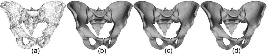
M. Kazhdan / Reconstruction of Solid Models

                                                                                               b = 32    b = 64      b = 128         Error
                                                                           N = 1000            0.43%     0.30%        0.29%          RMS
                                                                                               3.11%     2.35%        2.37%          Maximum

                                                                           N = 10, 000         0.32%     0.12%        0.06%          RMS
                                                                                               2.42%     1.17%        0.68%          Maximum

                                                                           N = 100, 000        0.31%     0.10%        0.04%          RMS
                                                                                               2.33%     0.70%        0.37%          Maximum

Figure 3: The original model from which the test samples were
obtained. The inset shows a view of the base of the model, indicating    Table 2: The distance, as a percentage of model size, of the initial
that the model is not water-tight.                                       model from the reconstructed surface as a function of the number of
                                                                         samples (N) and band-width (b).
                                                                            The computational complexity and the complexity of the
                                                                         reconstructed surfaces are described in Table 1. Because our
                                                                         reconstruction algorithm runs in O(b3 log(b) + N) time and
                                                                         because the triangle count is quadratic in the sampling reso-
                                                                         lution, we find that doubling the band-width results in com-
                                                                         putation time that is roughly eight times larger and a recon-
                                                                         structed model with four times the number of triangles. Ad-
                                                                         ditionally, the table highlights the fact the limiting factor in
                                                                         the reconstruction is the computation of the forward and in-
                                                                         verse Fourier transforms, so that changing the number of in-
                                                                         put samples does not markedly affect computation time.
                                                                            To evaluate how well our method reconstructs the sur-
                                                                         face of the model, we randomly sampled the initial model
                                                                         at 100, 000 points and computed the distance from these test
                                                                         points to the reconstructed models. Table 2 gives the accu-
                                                                         racy of the reconstructed models shown in Figures 4 in terms
                                                                         of the root mean square (RMS) and maximum distance of
Figure 4: Reconstructed surfaces of the Stanford bunny with differ-      these models from the test points (with the distance given as
ent numbers of surface samples (N) and different band-widths (b).        a percentage of the voxel resolution). As expected, the ta-
                                                                         ble indicates that the quality of the reconstruction improves
does not define a solid volume. The results of reconstruction            when the sample size and reconstruction band-width are in-
experiments at different sample sizes (N) and different band-            creased. The table also shows that the RMS errors does not
widths (b) are presented in Figure 4 and Tables 1 and 2.                 exceed the size of a voxel and, when the surface is recon-
   As Figure 4 indicates, our method returns a model that                structed at sufficiently high resolution, the maximum error is
approximates the input and smoothly fills in the holes where             also smaller than a voxel. Thus, our method provides a fast,
data is missing. The image also shows that the accuracy of               water-tight reconstruction, with sub-voxel accuracy. (Note
reconstruction increases with sample size and band-width.                that since the bunny model has holes, water-tight reconstruc-
                                                                         tions must introduce surface patches that are not present in
                                                                         the initial model. As a result, symmetrizing the error metric
                       b = 32          b = 64           b = 128          by sampling points on the reconstruction and measuring the
                                                                         distance to the initial model would result in an inaccurate
                     T =12, 384      T =51, 112      T =206, 448         measure of reconstruction accuracy.)
 N = 1000
                      s=0.16          s=1.07          s=8.05
                                                                            To evaluate the robustness of our method in the presence
                     T =11, 952      T =49, 776      T =201, 804         of larger aberrations, we ran our algorithm on an oriented
 N = 10, 000
                      s=0.18          s=1.11          s=8.04             point set that was uniformly sampled from part of a model of
                                                                         human head. Figure 5 shows the surface from which the sam-
                     T =11, 880      T =49, 508      T =200, 668
 N = 100, 000                                                            ples were taken (top row) and the reconstruction returned by
                      s=0.52          s=1.44          s=8.60
                                                                         our method (bottom row). In this experiment, the sample
                                                                         size was set to N = 100, 000 and the reconstruction band-
Table 1: The size T , in triangles, and compute time s, in seconds,      width was set to b = 128. Although the input samples only
for reconstruction of the Stanford bunny as a function of the number     come from a fraction of the surface, the figure shows that our
of samples (N) and band-width (b).
                                                                                                               c The Eurographics Association 2005.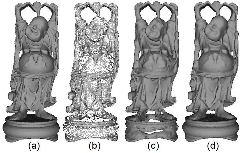
M. Kazhdan / Reconstruction of Solid Models

                                                                         Figure 6: The toes of Michelangelo’s David model (left) and the re-
                                                                         constructions obtained using uniform weights (middle) and weights
Figure 5: Reconstructed surfaces of a human face using samples           that are inversely proportional to the sampling density (right).
from a 3D model. Views of the original model are shown in the top
row. Views of the reconstructed, water-tight model are shown in the
bottom row.

method returns a solid model that accurately fits the input
samples while providing a reasonable reconstruction of the
surface in the regions where no samples could be provided.
   Figure 6 shows the reconstructions for a point set that was
uniformly sampled from the surface of the toes of Michelan-
gelo’s David model (N = 100, 000, b = 128). The initial
model is shown on the left, with a crack between the first two
toes resulting from the scanner’s inability to see the region.
Using our method to reconstruct the surface of the model by
assigning uniform weights to each sample point gives rise to
the surface shown in the middle column. While this surface               Figure 7: Reconstructions from a non-uniform point set. The ini-
accurately approximates the data and results in a water-tight            tial Buddha model (a), the point set sampled as a function of sur-
reconstruction, it introduces a topological handle connect-              face curvature (b), the reconstructed surface obtained using uniform
                                                                         point weighting (c), and the surface reconstructed using our weight
ing the first two toes. By assigning weights to the samples
                                                                         assignment method (d).
that are inversely proportional to the regional sampling den-
sity, as described in Section 3.5, we obtain a new reconstruc-           the reconstructions closely approximates the initial surface
tion (right column) that gives more weight to the points near            (Figure 7(a)), indicating that though our weight assignment
the boundary of the crack. This forces the reconstruction to             method is a heuristic, it gives a good approximation to the
maintain the surface orientation near the missing data and               true sampling density and results in robust reconstructions.
results in a reconstruction that does not have the topological
                                                                            Finally, to test how well our method performs in the pres-
artifact introduced when uniform weights are used.
                                                                         ence of noise, we sampled a cow model at 100,000 points
   To evaluate the performance of our method in the pres-                and added noise to both the position and normal of each
ence of non-uniform sampling, we generated an oriented                   sample. Noise was added to each sample by randomly dis-
point set by randomly sampling 100, 000 points from the sur-             placing the position by a fixed distance and randomly chang-
face of the “Happy Buddha” model, Figure 7(a), where the                 ing the direction of the normal by a fixed angle. The recon-
probability of choosing a point was a function of the sur-               structed cow models are shown in Figure 8. The rows show
face curvature. An image of the point set is shown in Fig-               the change in the reconstructed model as the positional noise
ure 7(b), with sparse sampling in low curvature regions (e.g.            is increased and the columns show the change as the angular
the stomach and the base of the pedestal) and dense sam-                 noise is increased. The results in the image indicate that our
pling in high curvature regions. Figure 7(c) shows the re-               reconstruction method is robust in the presence of both po-
construction obtained using uniform weighting which over-                sitional and angular error. In particular, the figure shows that
integrates the high curvature areas, resulting in a poor recon-          our method reconstructs all but the features of the model that
struction in planar regions. In contrast, Figure 7(d) shows the          are smaller than the displacement size. For example, when
reconstruction obtained when we use our weighting method                 a displacement value of 1/32-nd of the bounding radius is
to assign weights to the samples. As the figure indicates,               used (right column), the body of the cow is reconstructed,

c The Eurographics Association 2005.
M. Kazhdan / Reconstruction of Solid Models
convolution of the noise model with the implicit function ob-
tained from noise-free samples. For example, if the sampling
noise is Gaussian, the reconstructed characteristic function
of the noisy samples will approximate a smoothed version
of the characteristic function of the noise-free samples. As a
result, the surface reconstructed from samples with Gaussian
noise will resemble a smoothed version of the initial model.
4.3. Comparison to Related Methods
Our method differs from much of the previous work in sur-
face reconstruction in that the fitting of the reconstructed sur-
face to the samples requires a simple global optimization.
Specifically, due to the additive nature of the reconstruc-
tion process, we fit the characteristic function to the sam-
ple points on a point-by-point basis without considering the
proximity of adjacent points. Then, to extract the iso-surface,
we optimize by simply setting the iso-value equal to the av-
Figure 8: Reconstructions of a cow model where varying amounts
erage of the characteristic function at the sample points.
of noise were added to the position and the normals of the samples.
In order to evaluate the effects of our global optimization
but the legs and horns, whose widths are smaller the size of
on the accuracy of retrieval, we compared the reconstruc-
the displacement, can no longer be reconstructed. More im-
tions obtained using our method with the reconstructions
portantly, these results show that our method remains robust
obtained using Radial Basis Functions [CB∗ 01, RBF] and
in the presence of significant normal error. This is particu-
Multi-Level Partition of Unity Implicits [OB∗ 03, MPU].
larly important in practical settings, because though the po-
sitions of the sample points may be accurately obtained with To compare these methods we ran the reconstruction algo-
3D scanners, the normals, which are differential properties rithm on point sets obtained from water-tight models of a hu-
of the surface, are often more noisy. man pelvis and the Armadillo Man. In the first experiment,
the point sets were non-uniformly sampled from the surface
of the model and in the second experiment, the points were
4.2. Discussion
uniformly sampled from the surface of the model and then
4.2.1. Memory Requirements noise was added to the samples prior to the reconstruction.
The results of our experiments are shown in Figures 9 and 10
One limitation of our approach is its memory requirements.
and the complexity and accuracy of the reconstructions are
If we would like to obtain a high detail reconstruction of a
described in Table 3. In both experiments, the points sets
model, it is necessary to generate a large voxel grid. Specifi-
consisted of N = 100, 000 samples and the surfaces were re-
cally, if we would like to reconstruct a model at band-width
constructed at a band-width of b = 128. The accuracy of a re-
b it is necessary to perform forward and inverse FFTs on
construction was measured by uniformly sampling 100,000
a 2b × 2b × 2b voxel grid. Assuming that the values of the
points from both the initial model and the reconstructed sur-
voxels are stored at floating point precision this implies that,
face and computing the distances of the points sampled from
given the memory limitations of commodity computers, our
the initial surface to the reconstructed surface and the dis-
method cannot reconstruct a surfuce using a voxel grid with
tances of the points sampled from the reconstructed surface
resolution larger than 512 × 512 × 512.
to the initial surface.
4.2.2. Translation, Additivity, and Noise The results from the pelvis experiment demonstrate that
all three methods return accurate reconstructions of the
An important feature of our method is that it commutes with
model, despite the non-uniformity in the sampling and the
translation and is additive. That is, (1) the implicit function
large genus of the model. Furthermore, as the results in Ta-
obtained from a translated point set is equal to the transla-
ble 3 indicate, even though our optimization step is a simple
tion of the implicit function obtained from the initial point
averaging operation that results in faster reconstruction, the
set, and (2) the implicit function obtained from the union of
lack of explicit local optimizations does not give rise to a
two subsets is equal to the sum of the implicit functions ob-
less accurate reconstruction. Thus our method returns a re-
tained from each subset independently. A property that any
construction that has the same resolution and accuracy as
such method satisfies is that if we can model the noise acting
competing reconstructions but runs in less time.
on the samples by a probability distribution, then the implicit
function obtained from noisy samples will approximate the The difference in the approaches becomes amplified in the
c The Eurographics Association 2005.M. Kazhdan / Reconstruction of Solid Models
ficiently, making the Radial Basis Function reconstruction
run five times slower and the Partition of Unity reconstruc-
tion run three time slower. In contrast, the efficiency of our
method, which only performs a single averaging optimiza-
tion, is not affected by the noise in the data, returning an
Figure 9: A non-uniform sampling of points from the human pelvis accurate reconstruction in the same amount of time.
(a) and the reconstructions obtained using Radial Basis Functions
(b), Partition of Unity Implicits (c), and our method (d).
5. Conclusion and Future Work
In this paper we have presented a novel method for re-
constructing seamless meshes from oriented point samples.
Our method differs from past approaches in that it leverages
Stokes’ Theorem to provide a method for surface reconstruc-
tion that does not require the establishment of topological
relations between adjacent points and involves no implicit
parameter fitting. Consequently, we provide a surface recon-
struction method that is both simple and efficient. We have
shown that the method is robust and can be used to recon-
struct the surface of 3D solids in the presence of missing
data, non-uniform sampling, and noise.
Figure 10: The armadillo-man model (a) and reconstructions from In the future, we would like to consider using a method
a noisy point sample obtained using Radial Basis Functions (b), akin to PolyCube-Maps [TH∗ 04] to decompose the input
Partition of Unity Implicits (c), and our method (d). The inset shows samples into a collection of regionally localized subsets.
a magnification of the model’s face, showing that the local nature of This would enable us to run our method on each of the
previous reconstruction approaches results in noisy reconstructions. subsets independently, allowing us to overcome the mem-
ory bottleneck that restricts the resolution of reconstructable
Armadillo Man experiment when noise is added to the sam- detail. We expect that the additive nature of our reconstruc-
ples. In the results of this experiment, the local optimiza- tion process should facilitate this task by providing a method
tions of the Radial Basis Function and Partition of Unity ap- for stitching together adjacent reconstructions.
proaches give rise to surfaces that strive to interpolate the
samples and are themselves noisy. In contrast, the additive
nature of our method (as described in the previous section) References
gives rise to a surface reconstruction that averages out the [ABK98] A MENTA N., B ERN M., K AMVYSSELIS M.:
noise and returns a surface that resembles a smoothed ver- A new Voronoi-based surface reconstruction algorithm.
sion of the initial model and is, on average, about twice as Computer Graphics (Proceedings of SIGGRAPH 98)
accurate as the reconstruction of the competing methods. (1998), 415–21. 2
The local nature of the optimizations in the Radial Basis [AC∗ 00] A MENTA N., C HOI S., D EY T., L EEKHA N.: A
Function and Partition of Unity approaches is further high- simple algorithm for homeomorphic surface reconstruc-
lited by the timing results in Table 3. Since the input samples tion. ACM Symp. on Computational Geometry (2000),
are noisy, the iterative local optimizations converge less ef- 213–222. 2
[ACK01] A MENTA N., C HOI S., KOLLURI R.: Power
crust. 6th ACM Symp. on Solid Modeling and Applica-
tions (2001), 249–260. 2
Model Time Tris. RMS Max
[Bo84] B OISSONNAT J.: Geometric structures for three
RBF 5 : 23 302K 0.10% 2.19% dimensional shape representation. ACM TOG (1984),
Pelvis MPU 0 : 39 288K 0.12% 3.37% 266–286. 2
Ours 0 : 12 289K 0.11% 1.85%
[CB∗ 01] C ARR J., B EATSON R., C HERRIE H., MITCHEL
RBF 24 : 10 200K 0.13% 0.50% T., F RIGHT W., M C C ALLUM B., E VANS T.: Reconstruc-
Armadillo MPU 2 : 14 205K 1.16% 12.71% tion and representation of 3D objects with radial basis
Ours 0 : 11 176K 0.07% 0.67% functions. ACM SIGGRAPH (2001), 67–76. 2, 8
[CL96] C URLESS B., L EVOY M.: A volumetric method
Table 3: A comparison of the reconstruction time (min:sec), the for building complex models from range images. Com-
triangle count, and the accuracy of the reconstructions of the pelvis puter Graphics (Proceedings of SIGGRAPH 96) (1996),
and Armadillo Man models using Radial Basis Functions, Multi- 303–312. 2
Level Partition of Unity Implicits, and our method.
c The Eurographics Association 2005.M. Kazhdan / Reconstruction of Solid Models
[CM95] C HEN Y., M EDIONI G.: Description of complex In this appendix, we show that although there are many
objects from multiple range images using an inflating bal- complex vector functions whose divergences are equal to a
loon model. Computer Vision and Image Understanding given complex exponential, if we would like the reconstruc-
(1995), 325–334. 2 tion to satisfy two simple properties, these vector functions
[DG03] D EY T., G OSWAMI S.: Tight cocone: A water have to be unique. In particular, we show that if we would
tight surface reconstructor. In Proc. 8th ACM Symp. on like the reconstruction process to satisfy:
Solid Modeling Applications (2003), 127–134. 2 • The contribution of a point to the reconstructed implicit is
[DM∗ 02] DAVIS J., M ARSCHNER S., G ARR M., L EVOY independent of the contribution of any other point, and
M.: Filling holes in complex surfaces using volumetric • The reconstruction commutes with translation and rota-
diffusion. In Intl. Symp. on 3D Data Processing, Visual- tion (translations and rotations of the point set result in
ization and Transmission (2002), 428–438. 2 corresponding translations and rotations of the implicit)
[EM94] E DELSBRUNNER H., M ÜCKE E.: Three- then the vector function giving rise to the ~l-th Fourier coef-
dimensional alpha shapes. ACM TOG (1994), 43–72. 2 ficient can only be:
~F~ (~q) = i~l/k~lk2 e−ih~l,~qi .
[RBF] FAST RBF 1.4.1: http://www.farfield- l
technology.com/, 2004. 8 To prove this, we recall that given a point set {~pi ,~ni }, the
~l-th Fourier coefficient of the implicit function is defined by:
[FFTW] FFTW: http://www.fftw.org, 1998. 1
F̂(~l) = ∑i ~F~l (~pi ),~ni .
D E
[HD∗ 92] H OPPE H., D E ROSE T., D UCHAMP T., M C -
D ONALD J., S TUETZLE W.: Surface reconstruction from Since we assume that the contribution of any point is inde-
unorganized points. ACM SIGGRAPH (1992), 71–78. 2 pendent of any other point, it suffices to prove the uniqueness
property for the case when the point set consists of a single
[LC87] L ORENSEN W., C LINE H.: Marching cubes: A
oriented point {~p,~n}.
high resolution 3d surface reconstruction algorithm. SIG-
GRAPH Conference Proceedings (1987), 163–169. 1 The condition that the reconstructed function commutes
[MPU] MPU I MPLICITS: http:// www. mpi-sb. with translation implies that if F̂(~l) is the ~l-th Fourier co-
mpg.de/˜ohtake/mpu_implicits/. 8 efficient of the reconstruction obtained using the oriented
~
point {~p,~n}, then e−ihl,~p0 i F̂(~l) is the ~l-th Fourier coeffi-
[OB∗ 03] O HTAKE Y., B ELYAEV A., A LEXA M., T URK
cient of the reconstruction obtained using the oriented point
G., S EIDEL H.: Multi-level partition of unity implicits.
{~p + ~p0 ,~n}. Since this must be true for any normal vector
ACM TOG (2003), 463–470. 8
~n, it follows that the function ~F~l (~p) can be factored as the
[OBS04] O HTAKE Y., B ELYAEV A., S EIDEL H.: 3D scat- ~ ~l)e−ih~l,~pi with G(
~ ~l) ∈ C3 .
product ~F~ (~p) = G(
l
tered data approximation with adaptive compactly sup-
ported radial basis functions. SMI (2004), 31–39. 2 Moreover, since the divergence of ~F~l (~p) has to be equal to
[OF∗ 01] O SADA R., F UNKHOUSER T., C HAZELLE B., ~
e l,~pi , it follows that −ihG(
−ih ~ ~l),~li = 1. Thus, we know that:
D OBKIN D.: Matching 3d models with shape distribu- G(l) = i~l/k~lk2 +~l ⊥
~ ~ (2)
tions. SMI (2001) 154–166. 5 where l is a vector perpendicular to ~l.
~ ⊥
[TH∗ 04] TARINI M., H ORMANN K., C IGNONI P., M ON - Since we also want the reconstruction to commute with
TANI C.: Polycube-maps. TOG (SIGGRAPH 2004) rotation, this implies that if F̂(~l) is the ~l-th Fourier coeffi-
(2004), 853–860. 9 cient of the reconstruction obtained using the oriented point
[TO04] T URK G., O’B RIEN J.: Modelling with implicit {~p,~n}, then F̂(R(~l)) is the ~l-th Fourier coefficient of the re-
surfaces that interpolate. ACM TOG (2004), 855–873. 2 construction obtained using the oriented point {R(~p), R(~n)},
[TV91] T ERZOPOULOS D., VASILESCU M.: Sampling for any rotation R.
and reconstruction with adaptive meshes. In IEEE CVPR Thus, in order for the reconstruction process to commute
(1991), 70–75. 2 with rotation, the function G( ~ ~l) must satisfy the property:
[Wh98] W HITAKER R.: A level-set approach to 3d recon- ~ ~
R(G(l)) = G(R(~ ~l)).
struction from range data. IJCV (1998), 203–231. 2 Clearly, the function G(l) = il/k~lk2 satisfies this property.
~ ~ ~
On the other hand, if we take R to be a rotation about the
Apppendix vector ~l, we get R(G( ~ ~l)) = G(
~ ~l). Thus, it follows that ~l ⊥
(in Equation 2) must be zero, and hence the only function
To reconstruct a surface from an oriented point set, we com- satisfying translation and rotation commutativity is:
pute the Fourier coefficients of the characteristic function by
~F~ (q) = i~l/k~lk2 e−ih~l,~qi .
approximating surface integration by a Monte-Carlo summa- l
tion. To do this we need to define complex vector functions
whose divergences are equal to the complex exponentials.
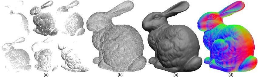
c The Eurographics Association 2005.M. Kazhdan / Reconstruction of Solid Models Figure 11: A reconstruction of the Stanford bunny model from range scans: Some of the initial scans of the model, obtained from different view points, are shown in (a). The complete point set, obtained by merging the scans, is shown in (b). The reconstructed surface is shown in (c). And a visualization of the surface, obtained by mapping the normal coordinates to RGB is shown in (d). Note that although the overlap of different scans results in a non-uniform distribution of points, our weighting scheme correctly assigns sampling densities to the input points, resulting in an accurate and smooth reconstruction of the surface (as demonstrated by the smooth variation of normals seen in (d)). (Model courtesy of Stanford University Computer Graphics Laboratory.) c The Eurographics Association 2005.
You can also read


