Novel Adaptive Binary Search Strategy-First Hybrid Pyramid- and Clustering-Based CNN Filter Pruning Method without Parameters Setting
←
→
Page content transcription
If your browser does not render page correctly, please read the page content below
Novel Adaptive Binary Search Strategy-First Hybrid Pyramid- and
                                             Clustering-Based CNN Filter Pruning Method without Parameters Setting

                                                                   Kuo-Liang Chung       Yu-Lun Chang        Bo-Wei Tsai
                                                                   National Taiwan University of Science and Technology
                                                                 Department of Computer Science & Information Engineering
                                                                             {klchung01, lance030201, haha4nima}@gmail.com
arXiv:2006.04451v1 [cs.CV] 8 Jun 2020

                                                                 Abstract                                    processor units (GPU) with efficient parallel, pipeline,
                                                                                                             and vectorization processing capabilities, several interest-
                                            Pruning redundant filters in CNN models has received             ing CNN models have been developed, such as VGG-16
                                        growing attention. In this paper, we propose an adaptive             [40], SegNet [2], AlexNet [27], GoogLeNet [41], GAN
                                        binary search-first hybrid pyramid- and clustering-based             (Generative Adversarial Network) [14], Mask-RCNN
                                        (ABSHPC-based) method for pruning filters automatically.             [17], U-Net [39], and so on. Among these developed
                                        In our method, for each convolutional layer, initially a             CNN models, some may need more than several giga
                                        hybrid pyramid data structure is constructed to store the            of parameters. However, some of these parameters are
                                        hierarchical information of each filter. Given a tolerant            redundant, which leads to the model compression study.
                                        accuracy loss, without parameters setting, we begin from             The compressed CNN models can thus be deployed into
                                        the last convolutional layer to the first layer; for each            resource constrained embedding systems, such as mobile
                                        considered layer with less or equal pruning rate relative to         phones and surveillance systems [6].
                                        its previous layer, our ABSHPC-based process is applied                 In the past years, many model compression methods
                                        to optimally partition all filters to clusters, where each           have been developed, including: (1) the weight prun-
                                        cluster is thus represented by the filter with the median root       ing approach, (2) the layer pruning approach, (3) the
                                        mean of the hybrid pyramid, leading to maximal removal               knowledge distillation approach, (4) the low-rank matrix
                                        of redundant filters. Based on the practical dataset and             factorization approach, and (5) the filter pruning approach.
                                        the CNN models, with higher accuracy, the thorough ex-               Two commonly used metrics to evaluate the model com-
                                        perimental results demonstrated the significant parameters           pression performance are the reduction rate of the number
                                        and floating-point operations reduction merits of the pro-           of parameters required in the compressed CNN model over
                                        posed filter pruning method relative to the state-of-the-art         the number of parameters required in the original CNN
                                        methods.                                                             model, simply called the parameters reduction rate, and the
                                                                                                             reduction rate of the number of floating-point operations
                                        1. INTRODUCTION                                                      (FLOPs) used over the number of FLOPs used in the
                                                                                                             original CNN model, simply called the FLOPs reduction
                                           Convolutional neural networks (CNN) have been widely              rate.
                                        used in developing deep learning models for many applica-               In the weight pruning approach [4], [15], [16], [20],
                                        tions in computer vision, image processing, compression,             [29], [40], [43], when one absolute weight value of the
                                        speech processing, medical diagnosis, and so on. LeCun               kernel in the filter is less than the specified threshold, it
                                        et al. [28] proposed the LeNet-5 model, which consists of            could be zeroized. However, due to the irregular weight
                                        three convolutional layers and two fully connected layers,           zeroization for each filter, it may need a sparse matrix
                                        for document recognition. Krizhevsky et al. [27] proposed            computation-supporting library to accelerate the related
                                        the AlexNet model consisting of five convolutional layers            convolutional operations. Alternatively, we can quantize
                                        and three fully-connected layers to solve the visual object          each weight value by limited precision, where a lookup
                                        recognition problem in the ImageNet challenge [11]. Their            table shared by all the filters is often used to map the
                                        AlexNet model needs a few million parameters (also called            quantized weight value to an optimized integer. In the
                                        weights).                                                            layer pruning approach [30], [6], [7], researchers suggested
                                           Due to the great technology achievement in graphics               pruning all the filters in the considered convolutional layer.

                                                                                                         1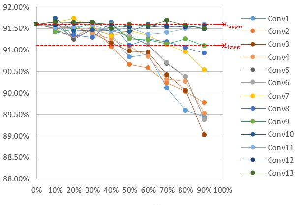
Chen and Zhao [7] analyzed the feature representations mental results demonstrated the accuracy merit of their
in different layers, and then a feature diagnosis approach method relative to other methods [26], [46]. Lin et al.
was proposed to prune unimportant layers. Finally, the [31] modeled the filter pruning problem as a minimization
compressed model was retrained by the knowledge distil- problem associated with an objective function problem to
lation technique [23] to compensate for the performance seek the best tradeoff between the filter selection and the
loss. Cheng et al. [8] pointed out that purely using the minimization of the cross-entropy loss for classification
knowledge distilling approach in model compression is not error between the labels of ground truth and the output of
suitable for solving the classification-oriented problems. the last layer in the considered CNN model. Luo et al. [37],
The low-rank factorization technique [12] was proposed [38] first calculated the sum of all entries of each channel
to decompose the weight matrix as a product of two smaller in the feature map produced by the ith convolutional
matrices by controlling the rank of the weight matrix such layer, and then they pruned the channel with the minimal
that many parameter values can be predicted, and then those sum. The pruning process is repeated until the specified
redundant parameter values can be pruned. Because more channel pruning rate is reached; the subsequent removal
and more 3x3 and 1x1 kernels have been used in the current of the corresponding filters in the ith and (i+1)th layers is
models [5], [45], it limits the parameters and FLOPs reduc- followed.
tion rates by the low-rank factorization technique. In He et al.s soft filter pruning (SFP) method [19],
Due to user accessibility and friendly tuning, the filter for the ith layer, they first sorted all filters in the layer
pruning approach provides the efficiency benefit on both according to their L2 -norm values. Next, according to a
CPU and GPU because no special hardware and/or library fixed pruning rate, namely 25% for the 1st-13th layers,
supports are required. In the next subsection, several i.e. Conv1-Conv13, they zeroized these filters with smaller
state-of-the-art filter pruning methods are introduced. L2 -norm values. In the next retraining step, all the deter-
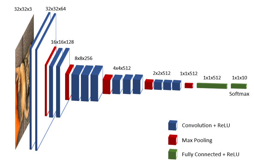
For easy exposition, we take VGG-16 (Visual Geometry mined filters including the zeroized filters are retrained.
Group-16) [42], as shown in Fig. 1, as the example in the Following the same pruning rate, the above step is repeated
introduction of the related work. In VGG-16, there are until the number of epochs has been reached. Finally, they
thirteen convolutional layers, namely Conv1-Conv13, and discarded those filters still with zero L2 -norm values. Their
one fully connected layer, namely Fc1. The configuration SFP method can not only be applied to maintain the model
of VGG-16 is shown in Table 1. capacity to achieve better model compression performance,
but it is also less dependent on the pre-trained model.
1.1. Related Work However, the same fixed pruning rate setting for each
In Li et al.’s method [30], for each convolution layer, convolutional layer limits the filter pruning performance.
they sorted all filters according to their absolute weight Due to the available code, the SFP method is included in
sums in increasing order. Next, based on a fixed filter the comparative methods.
pruning rate, namely 50%, for the 8th-13th layers, i.e. In [1], based on the cosine-based similarity metric to
Conv8-Conv13, and the first layer Conv1, they discarded measure the similarity level between two filter clusters
those filters with smaller absolute sums. However, due to in the ith layer, if the similarity value is larger than the
the fixed pruning rate setting, it limits the filter pruning specified distance threshold, namely 0.3 empirically, the
performance. Based on the filter sparsity concept in [34], two clusters are merged. Ayinde and Zurada [1] repeat
Liu et al. [33] defined a filter as being more redundant than their cosine-based merging method (CMM) until all similar
others when that filter has several coefficients which are clusters are merged. For each cluster, they randomly select
less than the mean value of all absolute filter weights in that one filter to represent that cluster and discard the remaining
layer. By using the rate-distortion optimization technique filters in that cluster. In addition, they remove the corre-
in image coding, they proposed a computation-performance sponding feature maps produced by those discarded filters
optimization approach to prune redundant filters. Due to in the ith layer; in the (i+1)th layer, they also discard the
the available code, Li et al.’s fixed pruning rate- and back- filters corresponding to the removed feature maps produced
ward pruning-based (FPBP-based) method [30], simply by the ith layer. However, the fixed distance threshold
called the FPBP method, is included in the comparative setting for determining the clusters for each convolutional
methods. layer limits the pruning performance. Due to the available
Given an allowable number of filters to be pruned code, the CMM method [1] is included in the comparative
for each layer, He et al. [22] considered the distortion methods.
between the original feature map and the resultant feature To improve the previous SFP method, He et al. [21]
map caused by the pruning filters, and then they derived a proposed a geometric median-based filter pruning (GMFP)
1-norm regularization formula to model the filter pruning method. For the considered layer with k filters, they first
problem as a constraint minimization problem. Experi- calculate the geometric center of all the filters in that layer,
2where the sum of all distances between each filter and In the third contribution, for the next convolutional
the geometric center is the smallest among that for the layer, namely Conv12, the initial pruning rate of Conv12,
other location. Then, according to a specified pruning namely α12 , is equal to α13 . Based on this initial pruning
rate, namely 30% for layers 1-13, they zeroize the k*30% rate α12 and the same allowable accuracy loss of 0.5%,
filters which are closest to the geometric center. In the the proposed ABSHPC-based filter pruning process is
subsequent retraining step, all the filters are retained. The applied to discard the redundant filters in Conv12 as much
above GMFP process and the retraining step are repeated as possible. Empirically, it yields α12 = 87.5%. We repeat
until the required number of epochs has been reached. The the above ABSHPC-based filter pruning processes for
experimental results justified better parameters and FLOPs Conv11, Conv10, Conv9, ..., Conv2, and Conv1, where
reduction merits by the GMFP method relative to the SFP the resultant eleven filter pruning rates are 87.5%, 87.5%,
method [19]. However, the fixed pruning rate setting for 62.5%, 62.5%, 50.5625%, 31.25%, 31.25%, 0%, 0%, 0%,
discarding redundant filters for each convolutional layer and 0%, respectively.
limits the pruning performance. Due to the available codes, In the fourth contribution, with the highest accuracy, the
the GMFP method is included in the comparative methods. parameters reduction rate gains of our filter pruning method
over the four state-of-the-art methods, namely the FPBP
1.2. Motivation method [30], the SFP method [19], the CMM method [1],
The above-mentioned limitation existing in the related and the GMFP method [21], are 24.35%, 44.55%, 24.67%,
filter pruning work prompted us to develop an automati- and 37.94%, respectively; the FLOPs reduction rate gains
cally adaptive filter pruning method to achieve significant of our method over the four methods are 17.78%, 8.33%,
reduction of parameters and FLOPs required in the CNN 7.93%, and 1.46%, respectively. In addition, based on the
models relative to the related state-of-the-art methods. same dataset on AlexNet [27], our method also achieves
substantial parameters and FLOPs reduction merits when
1.3. Contributions compared with the related methods.
In this paper, without parameters setting, we propose an The rest of this paper is organized as follows. In Section
automatically adaptive binary search-first hybrid pyramid- II, three observations on the accuracy-pruning rate curves
and clustering-based (ABSHPC-based) filter pruning method for all convolutional layers are delivered. In Section III,
to effectively remove redundant filters for CNNs, achieving the HP data structure is proposed to store the hierarchical
significant parameters reduction and FLOPs reduction information of each filter. Then, a fast HP-based closest
effects. The four contributions of this paper are clarified as filter finding operation is proposed. In Section IV, the
follows. proposed ABSHPC-based filter pruning process for each
In the first contribution, given an allowable accuracy convolutional layer is presented. Then, the whole proce-
loss, namely 0.5%, based on the CIFAR-10, we take dure of our filter pruning method is described. In Section V,
VGG-16 as the representative CNN model. From the the thorough experimental results are illustrated to justify
constructed accuracy-pruning rate curves shown in Fig. 2, the parameters and FLOPs reduction merits of our filter
three observations are delivered, and these observations pruning method. In Section VI, some concluding remarks
prompted us to prune filters following the order from the are addressed.
last convolutional layer to the first layer. According to this
backward pruning order, without parameters setting, we 2. THREE OBSERVATIONS ON THE CON-
propose an automatically adaptive filter pruning method STRUCTED ACCURACY-PRUNING RATE
such that the pruning rates comply with a decreasing CURVES
sequence.
In the second contribution, we propose a novel hybrid Based on the CIFAR-10 dataset, in which 50000 32x32
pyramid (HP) data structure to store the hierarchical infor- images are used as the training set and the disjoint 10000
mation of each filter in the considered convolutional layer, 32x32 images are used as the testing set, and VGG-16,
where the root mean of HP indicates the absolute sum of based on our experiments with 20 epochs, three observa-
the absolute weights of that filter, and then all HPs in the tions on the constructed accuracy-pruning rate curves are
considered layer are sorted in increasing order based on presented.
their root means. Futhormore, for the considered layer, un- According to the ten pruning rates [30], namely 0%,
der the same accuracy loss, we propose an ABSHPC-based 10%, 20%, 30%, ..., and 90%, for each convolutional layer
filter pruning process to remove the redundant filters to while retaining all the filters for the other twelve layers
achieve the maximal pruning rate. Empirically, our method each time. Based on the above pruning rates setting, the
begins with the 13th convolutional layer Conv13, and the filters with low absolute sums are pruned first. As a result,
maximal pruning rate of this layer is α13 = 87.5%. the thirteen accuracy-pruning rate curves are depicted
3Table 1.
THE CONFIGURATION OF THE THIRTEEN
CONVOLUTIONAL LAYERS IN VGG-16.
Layer Filter (#Filters) Feature Map
Conv1 3x3x3 (64) 32x32x64
Conv2 3x3x64 (64) 32x32x64
Maxpool - 16x16x64
Conv3 3x3x64 (128) 16x16x128
Conv4 3x3x128 (128) 16x16x128
Maxpool - 8x8x128
Conv5 3x3x128 (256) 8x8x256
Figure 1. The VGG-16 model. Conv6 3x3x256 (256) 8x8x256
Conv7 3x3x256 (256) 8x8x256
Maxpool - 4x4x256
Conv8 3x3x256 (512) 4x4x512
Conv9 3x3x512 (512) 4x4x512
Conv10 3x3x512 (512) 4x4x512
Maxpool - 2x2x512
Conv11 3x3x512 (512) 2x2x512
Conv12 3x3x512 (512) 2x2x512
Conv13 3x3x512 (512) 2x2x512
Maxpool - 1x1x512
Fc1 - 1x1x512
Fc2 - 1x1x10
3. HYBRID PYRAMID-BASED FILTER REP-
Figure 2. The accuracy-pruning rate curves of the thirteen convo- RESENTATION AND THE CLOSEST
lutional layers for VGG-16 and CIFAR-10.
FILTER FINDING OPERATION
In this section, we first propose a HP data structure
in Fig. 2 in which the X-axis denotes the pruning rate to store the hierarchical information of each filter in the
and the Y-axis denotes the accuracy value. Note that convolutional layer. Next, based on the proposed HP data
without pruning any filters for each convolutional layer, structure, some inequalities are derived to explain why
the classification accuracy of the trained VGG-16 model is given a filter as a key, its closest filter in a considered filter
91.60%, as depicted by the dashed line Lupper of Fig. 2, set can be found quickly. Note that the closest filter finding
indicating the accuracy upper bound. operation plays an important role in the proposed HP-based
Suppose the accuracy loss is 0.5%. As depicted in Fig. clustering process, which will be presented in Section IV.A.
2, the dashed line Llower denotes the accuracy lower bound
3.1. Hybrid Pyramid-Based Filter Representation
91.10% (= 91.60% - 0.5%). From Fig. 2 and the visual
help of Llower and Lupper , three new observations are 1) Constructing HP for each filter: We first take the 13th
given; they are: (1) the seven convolutional layers, Conv7, convolutional layer, namely Conv13, as the example to ex-
Conv8, Conv9, Conv10, Conv11, Conv12, and Conv13, plain how to construct the HP data structure to represent the
form a group and each of them can tolerate higher pruning hierarchical information of each filter in Conv13. Our pro-
rates rather than the other layers, even more than the filter posed HP is different from the Laplacian pyramid and the
pruning rate 50% used in [30], (2) instead of setting a zero quadtree pyramid [3], [29], [32] used in coding.
pruning rate for Conv6-Conv2 [30], nonzero pruning rates In Table 1, Conv13 consists of 512 3x3x512 filters,
can be considered for these layers, (3) for Conv13-Conv1, where each contains 512 channels in which each channel is
their filter pruning rates could form a decreasing sequence. exactly a 3x3 kernel. Initially, we take absolute operation
4on each weight in the filter to make the weight value non-
negative. For each filter, the 512 3x3 kernels are denoted
by K1 , K2 , ..., and K512 . Among the 512 kernels, the
former 256 kernels, K1 , K2 , ..., and K256 , form a square
48x48 matrix, denoted by Ml , in which the first kernel K1
is located at the top-left corner of Ml and the kernel K256
is located at the bottom-right corner. In the same way,
the latter 256 kernels, K257 , K258 , ..., and K512 , form a
square 48x48 matrix, where the kernels K257 and K512
are located at the top-left and bottom-right corners of Mr ,
respectively. The 48x48 matrix Ml constitutes the base of
the left sub-pyramid Pl , as shown in Fig. 3(a); Mr con-
stitutes the base of the right sub-pyramid Pr . Connecting
the two sub-pyramids, Pl and Pr , the constructed HP for
representing each 3x3x512 filter is depicted in Fig. 3(b).
As depicted in Fig. 3(a), the left sub-pyramid Pl consists
of six levels, Pl0 , Pl1 , ..., and Pl5 , where the fifth level Pl5
denotes the 48x48 matrix Ml , forming the base of Pl ; after
averaging each 3x3 sub-matrix of Pl5 to a mean value,
the 4th level Pl4 is constructed to store the condensed
16x16 matrix; the root level Pl0 saves the absolute mean
value of Pl5 . In the same way, the right sub-pyramid Pr
is constructed to store the hierarchical information of the
considered 3x3x256 filter. Finally, the roots of Pl and
Pr , i.e. Pl0 and Pr0 , are connected by a common root to
construct a hybrid pyramid. Fig. 3(b) depicts the resultant
HP for saving the hierarchical information of each 3x3x512 Figure 3. The constructed hybrid pyramid for each 3x3x512 filter.
(a) The constructed left sub-pyramid Pl for the 48x48 matrix con-
filter in Conv13.
verted from the former 256 3x3 kernels in the filter. (b) The con-
2) Computational complexity analysis and the sorted structed hybrid pyramid P by connecting the two sub-pyramids Pl
HPs for all filters in the layer: We first analyze the compu- and Pr .
tational complexity for constructing the hybrid pyramid of
each filter in Conv13, and then analyze the computational
complexity for constructing the sorted HPs. the HPs with the second smallest and the largest root means
For the fifth level of Pl , namely Pl5 , its size is N 2 = 482 . are 7 and 2 corresponding to P [7] and P [2], respectively.
In terms of the big-O complexity notation [10], it is not hard Considering the inverse of S[i] (= j), we build up the array
to verify that it takes O(N 2 ) (= 4/3*N 2 + constant) time to O[j] (= i) to access the sorted order of the hybrid pyramid
construct the sub-pyramid Pl . Similarly, it takes O(N 2 ) P [j], 1 ≤ j ≤ 512. Following the above three examples, we
time to construct Pr . Consequently, it takes O(N 2 ) time to have O[2] = 512, O[5] =1, and O[7] = 2.
construct the HP, as depicted in Fig. 3(b), for saving the According to Table 1 for VGG-16, the number of the
hierarchical information of each 3x3x512 filter in Conv13. constructed HPs for all the filters in each convolutional
According to the above HP construction method for each layer and the number of levels required for each HP are
filter, the constructed 512 HPs for the 512 filters in Conv13 tabulated in Table 2, in which “#(Hybrid Pyramids)”
are depicted in Fig. 4, where the 512 HPs are denoted by denotes the number of HPs required in each convolutional
P [1], P[2], ..., and P [512] corresponding to the filters F [1], layer and “#(Levels)” denotes the number of levels required
F [2], ..., and F [512], respectively. for each constructed HP.
According to the 512 root means of P [1], P [2], ..., and 3.2. Fast Hybrid Pyramid-Based Closest Filter
P [512], the 512 HPs are sorted in increasing order; S[i], 1 ≤ Finding
i ≤ 512, saves the original index of the sorted HP which is
in the ith place. This above sorting job can be done in O(|F| In this subsection, based on the sorted HPs for the
log |F|) time, where F ={F [1], F [2], ..., F [512]} and |F| (= considered convolutional layer, given a filter F [i] as a
512). As shown in Fig. 4, S[1] = 5 indicates that the index key, some inequalities are first derived to assist in quickly
of the HP with the smallest root mean is 5 corresponding to finding its closest filter in the considered filter set.
P [5]; S[2] = 7 and S[512] = 2” indicate that the indices of 1) Proof of inequalities and its application to prune
5calculate its true L2 -norm squared distance value.
We now extend Lemma 1 to derive the inequalities for
the same level between two hybrid pyramids to prune the
unnecessary L2 -norm squared distance calculation between
F [i] and F [j] in a top-down manner, achieving fast closest
filter finding of F [i] in the considered filter set.
From Table 2, each of the five convolutional layers,
Conv9-Conv13, has the same number of HPs, namely
512, and each HP has seven levels. Similar to the proving
technique for Lemma 1, we have a more general result.
Theorem 1. For the 9th-13th convolutional layers of VGG-
16, we have the following inequalities:
2 ∗ 44 ∗ 9 ∗ d2 (P 0 [i], P 0 [j]) ≤
Figure 4. The constructed hybrid pyramids for the 512 3x3x512
filters in the 13th convolutional layer of VGG-16. 44 ∗ 9 ∗ d2 ((Pl0 [i], Pr0 [i]), (Pl0 [j], Pr0 [j])) ≤
(1)
43 ∗ 9 ∗ d2 ((Pl1 [i], Pr1 [i]), (Pl1 [j], Pr1 [j])) ≤ ... ≤
Table 2.
THE NUMBER OF HYBRID PYRAMIDS AND LEVELS FOR d2 ((Pl5 [i], Pr5 [i]), (Pl5 [j], Pr5 [j]))
EACH CONVOLUTIONAL LAYER IN VGG-16.
Proof. See Appendix II.
Layer No. #(Hybrid Pyramids) #(Levels)
1 64 2
2 64 5 We also explain the physical meaning behind Theorem 1
3 128 5 by one example. Let the considered filter set be denoted
by F0 and let the temporary closest filter of F [i] be F [k]
4 128 6
∈ F0 . Let the L2 -norm squared distance between F [i]
5 256 6 and F [k] be 16384. We now examine whether the other
6-7 256 6 filter F [j] ∈ F0 can replace F [k] as a better closest filter
8 512 6 candidate of F [i]. Assume the L2 -norm square distance
between the root mean of P [i] and the root mean of P [j]
9-13 512 7
is 4, i.e. d2 (P 0 [i], P 0 [j]) = 4, and then we immediately
know 2 ∗ 44 ∗ 9 ∗ d2 (P 0 [i], P 0 [j]) = 2 ∗ 44 ∗ 9 ∗ 4 = 18432.
unnecessary L2 -norm distance calculations between two Because of d2 (F [i], F [k]) = 16384 ¡ 2 ∗ 44 ∗ 9 ∗ d2 (P 0 [i],
filters: Given a 3x3x512 filter F [i] as a key corresponding P 0 [j]) = 18432, by Theorem 1, we know that theoretically,
to the hybrid pyramid P [i], let the root mean of P [i] be the L2 -norm squared distance d2 ((Pl5 [i], Pr5 [i]), (Pl5 [j],
denoted by P 0 [i] which is equal to the mean of the two root Pr5 [j])) is always larger than or equal to 2 ∗ 44 ∗ 9 ∗ d2 (P 0 [i],
means Pl0 [i] and Pr0 [i]. Let the L2 -norm squared distance P 0 [j]) = 18432, so we ignore the true squared distance
between P 0 [i] and P 0 [j] be denoted by d2 (P 0 [i], P 0 [j]) calculation for d2 ((Pl5 [i], Pr5 [i]), (Pl5 [j], Pr5 [j])) because
where P 0 [j] denotes the root mean of a possible closest the filter F [j] has no chance of being a better closest
3x3x512 filter candidate F [j] in the considered filter set filter of F [i] relative to F [k], leading to the computation
with respect to F [i]. We have the following inequality. reduction effect.
After discussing how to apply Theorem 1 to reduce the
Lemma 1. 2*d2 (P 0 [i], P 0 [j]) ≤ d2 ((Pl0 [i], Pr0 [i]), (Pl0 [j], computational complexity of the L2 -norm squared distance
Pr0 [j]). calculation between two filters in the closest filter finding
for the kth, 9 ≤ k ≤ 13, convolutional layer, we now derive
Proof. See Appendix I. the inequalities for the kth, 6 ≤ k ≤ 8, convolutional layer;
as listed in Table 2, the constructed hybrid pyramid for each
The physical meaning behind Lemma 1 can be high- 3x3x256 filter is the same as in Fig. 3(a). In the same way,
lighted by an example. For example, suppose the L2 -norm for any two filters F [i] and F [j] in the kth layer, it yields
squared distance d2 (P 0 [i], P 0 [j]) is equal to 4, and then
the value of 2 ∗ d2 (P 0 [i], P 0 [j]) is equal to 8. By Lemma 1,
theoretically, the value of d2 ((Pl0 [i], Pr0 [i]), (Pl0 [j], Pr0 [j])) 44 ∗ 9 ∗ d2 (P 0 [i], P 0 [j]) ≤ 43 ∗ 9 ∗ d2 (P 1 [i], P 1 [j])
(2)
must be larger than or equal to 8, even though we do not ≤ ... ≤ d2 (P 5 [i], P 5 [j])
6Table 3. by computing the L2 -norm squared distance between the
THE DERIVED INEQUALITIES FOR EACH
base of the HP of F [i] and the base of the HP of F 0 [S[k]] as
CONVOLUTIONAL LAYER IN VGG-16.
the temporary minimum distance, denoted by d2min .
Layer No. Inequalities In the second step, for any other filter candidate F 0 [S[m]],
1 Eq. (5) m 6= k, in F0 , corresponding to the hybrid pyramid P 0 [S[m]],
2-3 Eq. (4) we further want to find the closest filter of F [i] in a smaller
4-5 Eq. (3) filter set instead of examining all filters in F0 - {F 0 [S[k]]}.
In what follows, we explain how to modify Theorem
6-8 Eq. (2) 1 to derive a smaller search range for further reducing
9-13 Eq. (1) the number of filter candidates to be examined. When
compared with the temporary minimum distance dmin ,
by Theorem 1, the closest filter candidate of F [i], namely
F 0 [S[m]], must satisfy the following inequality:
Similarly, in the kth, 4 ≤ k ≤ 5, convolutional layer, for
any two 3x3x128 filters, F [i] and F [j], we have d2min ≥ 2 ∗ 44 ∗ 9 ∗ d2 (P 0 [i], P 00 [S(m)])
(6)
= 2 ∗ 44 ∗ 9 ∗ (P 0 [i] − P 00 [S(m)])2
2 ∗ 43 ∗ 9 ∗ d2 (P 0 [i], P 0 [j]) ≤ 43 ∗ 9 ∗ d2 (P 1 [i], P 1 [j])
≤ ... ≤ d2 (P 4 [i], P 4 [j])
(3)
where P 00 [S(m)] denotes the root mean of the hybrid
pyramid of F 0 [S[m]]; P 0 [i] denotes the root mean of the
For any two 3x3x64 filters, F [i] and F [j], in the kth, 2 hybrid pyramid of F [i].
≤ k ≤ 3, convolutional layer, we have We first divide both sides of Eq. (6) by 2 ∗ 44 ∗ 9,
and then we take the square root operation on both sides.
Considering the two possible cases, (P 0 [i]- P 00 [S(m)] ≥ 0)
43 ∗ 9 ∗ d2 (P 0 [i], P 0 [j]) ≤ 42 ∗ 9 ∗ d2 (P 1 [i], P 1 [j])
(4) or (P 0 [i] - P 00 [S(m)] ≤ 0), the smaller search range of the
≤ ... ≤ d2 (P 4 [i], P 4 [j]) promising closest hybrid pyramids for F [i] corresponding
to the hybrid pyramid P [i] is thus bounded by
Finally, for any two 3x3x3 filters, F [i] and F [j], in the first
convolutional layer, we have
dmin
27 ∗ d2 (P 0 [i], P 0 [j]) ≤ d2 (P 1 [i], P 1 [j]) (5) (P 0 [i] − √ )≤
2 ∗ 42 ∗ 3
(7)
In terms of equation number, Table 3 tabulates the gen- dmin
P 00 [S(m)] ≤ (P 0 [i] + √ )
eral inequalities for each convolutional layer in VGG-16, 2 ∗ 42 ∗ 3
and these inequalities can be used to prune unnecessary
calculations in the proposed HP-based closest filter finding
operation.
2) The proposed hybrid pyramid-based closest filter The range in Eq. (7) is used to narrow the search range
finding operation: We still take Conv13 as the layer exam- for finding the closest filter of F [i]. On the other hand, if
ple. Given a filter F [i] in that layer as the key and under the root mean of one filter F 0 [S[m]] is out of the search
the considered filter set F0 , the proposed fast closest filter range in Eq. (7), F 0 [S[m]] will be viewed as a useless
finding operation wants to find the closest filter F [j] in F0 filter and will be kicked out immediately; otherwise, it
such that the L2 -norm squared distance between F [i] and goes downward to the next level of both hybrid pyramids
F [j] is the smallest. P [i] and P 0 [S[m]] and checks whether the filter F 0 [S[m]]
In the first step, all the HPs of the filters in F0 are sorted should be rejected or should go downward to the next
in increasing order based on their root means, and the sorted level. When it goes downward to the bottom level and the
HPs are corresponding to these filters F 0 [S[1]], F 0 [S[2]], ..., L2 -norm squared distance between the two related bases
and F 0 [S[|F’|]]. Given the root mean of the HP of F [i] as a is less than d2min , then the previous closest filter candidate
key, according to the binary search process, we can quickly F [S[k]] is replaced by the current filter F 0 [S[m]] as the
find the closest root mean of the HP of F 0 [S[k]] ∈ F0 . Next, new closest filter candidate to F [i]. We repeat the above
the squared distance between F [i] and F 0 [S[k]] is obtained step until the true closest filter of F [i] is found.
74. THE PROPOSED AUTOMATICALLY
Procedure: Automatical ABSHPC-Based Filter Pruning
ADAPTIVE BINARY SEARCH-FIRST
Input: Training set CIFAR-10, Trained VGG-16 with the
HYBRID PYRAMID- AND CLUSTERING-
accuracy 91.60%, and the allowable accuracy loss
BASED FILTER PRUNING METHOD 0.5%.
We first present the proposed HP-based clustering pro- Output: Compressed VGG-16.
cess, in which our HP-based closest filter finding operation
Step 1. (initialization for binary search) Perform k :=
is used as a subroutine. Secondly, without parameters set- (13) (13) (1)
ting, we present the whole procedure of the proposed auto- 13, Rupper := 1, Rlower := 0, R(13) := 0, Rupper
(1)
matical ABSHPC-based filter pruning method. := 1, Rlower := 0, and R(1) := 0.
4.1. The Proposed Hybrid Pyramid-Based Cluster- Step 2. (construct the sorted hybrid pyramids for the
ing Process kth layer) Construct the HP for each filter in the
kth convolutional layer. Next, sort all these HPs in
In the considered convolutional layer, let the currently increasing order based on their root means. Let the
considered filter set be denoted by F̄ . Suppose the filter initial set of all filters in the kth layer be denoted
pruning rate of this layer is |F̄c | . On the other hand, the goal by F (k) and let N (k) (= |F (k) |) denote the number
of the proposed HP-based clustering process is to partition of all filters in the kth layer.
all the filters in F̄ into c clusters such that one suitable
filter in each cluster is selected as the representative of that Step 3. (For 12 ≥ k ≥ 1, based on the pruning rate
cluster, achieving the filter pruning effect. passed by the last layer, perform the HP-based
First, we randomly select c filters from F̄ as the initial filter pruning process once) If k = 13, go to
c clusters, denoted by F̄ c , where each cluster contains only Step 4; otherwise, based on the pruning rate R(k)
(k+1)
one selected filter. We take each filter F [i] in F̄ - F̄ c as := |F |
obtained in the last convolutional
N (k+1)
a key, and then using the proposed HP-based closest filter layer, we apply the proposed HP-based clustering
finding operation, which has been described in Subsection process to partition the current filter set F (k) into
III.B.2, we can quickly find the closest filter of F [i], namely c (= R(k) |F (k) |) clusters. For each cluster, we
F [j] in F̄ c . select its representative filter with the median root
Next, we group those filters belonging to the same clus- mean and discard the other filters in that cluster.
ter as a new cluster, and then for each new cluster, the filter Let all the representatives of the c clusters be
with the median root mean of the hybrid pyramid is selected denoted by F (k) . After retraining VGG-16 based
as the representative filter of that cluster. Therefore, each on the current filter set F (k) in the kth layer and
cluster is represented by such a representative filter, and we the stationary filters in the other layers, if the
discard the other filters in that cluster. On the other hand, (k)
accuracy loss is larger than 0.5%, we set Rupper :=
each cluster now contains only one representative filter. In (k+1)
1 and Rlower := |F |
(k)
N (k+1)
, conceptually moving the
our experience, instead of taking the mean filter of all fil-
current binary search cursor to the right to increase
ters in that cluster as the representative, the above median
the number of representative filters, and go to Step
root mean-oriented selection strategy has better filter prun-
4; otherwise, go to Step 5.
ing performance due to the selection of the highly distinc-
tive representative. After reconstructing the c clusters via Step 4. (Adaptive binary search-first HP-based filter
these c representative filters, we repeat the above clustering (k) R(k) +R
(k)
pruning) Let Rold := R(k) and R(k) := upper 2 lower .
process to refine the c clusters until there is no change to the (k)
representative of each cluster. Finally, in these convergent c If |Rold - R(k) | is less than 0.0125, it means that
clusters, for each cluster, we take the filter with the median the binary search process has been done for six
root mean as the representative of that cluster, and prune the rounds, and then we go to Step. 5; otherwise, we
other filters in that cluster. apply the HP-based clustering process to partition
the current filter set F (k) into c (=R(k) |F (k) |) clus-
4.2. The Whole Procedure of the Proposed Au- ters. For each cluster, we select its representative
tomatical ABSHPC-Based Filter Pruning filter and discard the other filters in that cluster.
Method Let the set of these representatives of the c clusters
After presenting our HP-based clustering process, we still be denoted by F (k) . After retraining VGG-16
now present the proposed automatical ABSHPC-based based on F (k) and the stationary filters in the other
filter pruning method for the thirteen convolutional layers layers, if the accuracy loss is larger than 0.5%,
(k) (k)
(k) Rupper +Rlower
in VGG-16 and the whole procedure is shown below. we perform Rlower := 2 to move
8the current binary search cursor to the right to 5.2. The Parameters and FLOPs Reduction Merits
increase the number of representative filters in the for AlexNet
next round, and then we go to Step 4; otherwise,
R(k) +R
(k) We first outline the configuration of AlexNet. Next,
(k)
we perform Rupper := upper 2 lower to move the for each convolutional layer, the number of HPs and the
current binary search cursor to the left to decrease number of levels of each HP is analyzed. Furthermore,
the number of the representative filters in the next the inequalities for each convolutional layer are provided.
round and go to Step 4. Finally, the parameters and FLOPs reduction merits of our
ABSHPC-Based filter pruning method are demonstrated.
Step 5. (termination test) If k = 1, we report the com-
1) The configuration of AlexNet: AlexNet consists of five
pressed VGG-16 as the output and stop the proce-
convolutional layers and two fully connected layers. Table 6
dure; otherwise, we perform k := k − 1 and go to
tabulates the configuration of AlexNet in which there are 96
Step 2.
filters, each filter with size 11 × 11 × 3, in Conv1; there are
256 filters, each filter with size 5 × 5 × 96, in Conv2; there
are 384 filters, each filter with size 3 × 3 × 256, in Conv3;
5. EXPERIMENTAL RESULTS there are 384 filters, each filter with size 3 × 3 × 384, in
Conv4; there are 256 filters, each filter with size 3×3×384,
Based on the CIFAR-10 dataset and the two CNN in Conv5.
models, VGG-16 and AlexNet, the comprehensive experi- 2) The number of hybrid pyramids and the number of
ments are carried out to show the parameters and FLOPs levels of each HP in each convolutional layer: According
reduction merits of our automatical ABSHPC-based filter to the configuration of AlexNet, as shown in Table 6, the
pruning method relative to the state-of-the-art methods. number of the constructed HPs for all the filters in each
Under the Windows 10 platform, the source code of our convolutional layer and the number of levels required for
filter pruning method is implemented by Python language each HP are tabulated in Table 7.
and can be accessed from [13]. For the first layer, it is known that the number of HPs
All experiments are implemented using a desktop with required for the first layer is 96, and each filter is of size
an Intel Core i7-7700 CPU running at 3.6 GHz with 24 GB 11 × 11×3; the HP data structure of each filter connects
RAM and a Nvidia 1080Ti GPU. The operating system is three sub-HPs in which the base of each is a 11 × 11 matrix.
Microsoft Windows 10 64-bit. The program development Therefore, the level of each HP is three. For the second
environment is the Python programming language. layer, the number of HPs required for the second layer is
256, and each filter is of size 5×5×96; the HP data structure
of each filter connects six sub-HPs in which the base of each
5.1. The Parameters and FLOPs Reduction Merits
sub-HP is a (22 ×5)×(22 × 5) matrix. Therefore, the level
for VGG-16
of each HP is five. To reduce the paper length, we omit the
Table 4 tabulates the parameters and FLOPs reduction related discussion for Conv3-Conv5.
rates comparison among our ABSHPC-based filter pruning 3) The inequalities for each convolutional layer: In
method and the four state-of-the-art methods [1], [19], [21], terms of equation number, Table 8 tabulates the derived
[30]. In detail, Table 5 tabulates the filter pruning rate of inequalities for each convolutional layer in AlexNet, and
each convolutional layer by each considered method. these inequalities can be used to prune unnecessary cal-
Table 4 indicates that by the baseline method without culations in the proposed ABSHPC-based filter pruning
pruning any filters, the number of required parameters, method.
denoted by #(Parameters), the number of required FLOPs, Considering the first layer, from the constructed HP of
denoted by #(FLOPs), and the accuracy are 14.90M, each filter and the number of levels of each HP, as shown in
626.90M, and 91.60%, respectively. In Table 4, with the Table 7, according to the similar proving technique used in
highest accuracy and the lowest accuracy loss, our filter Theorem 1, we have the following inequalities:
pruning method has the highest parameters and FLOPs
reduction rates in boldface relative to the four state-of-the-
3 ∗ 112 ∗ d2 (P 0 [i], P 0 [j]) ≤
art methods. In detail, the parameters reduction rate gains
of our method over FPBP [30], SPF [19], CMM [1], and 112 ∗ d2 ((P10 [i], P20 [i], P30 [i]), (P10 [j], P20 [j], P30 [j])) ≤
GMFP [21] are 24.35%, 44.55%, 24.67%, and 37.94%, d2 ((P11 [i], P21 [i], P31 [i]), (P11 [j], P21 [j], P31 [j]))
respectively; the FLOPs reduction rate gains of our method (8)
over the four state-of-the-art methods are 17.78%, 8.33%, In the same way, for the second, third, fourth, and fifth
7.93%, and 1.46%, respectively. layers, the corresponding inequalities are given in Eq. (9),
Eq. (10), Eq. (11), and Eq. (11), respectively.
9Table 4. THE PARAMETERS AND FLOPS REDUCTION MERITS OF THE PROPOSED METHOD FOR VGG-16.
Parameters FLOPs
Method #(Parameters) #(FLOPs) Accuracy Accuracy loss
Reduction Rate Reduction Rate
Baseline 14.90M 0% 626.90M 0% 91.60% 0%
FPBP [30] 5.36M 64.00% 412.5M 34.20% 91.53% 0.07%
CMM [1] 5.41M 63.68% 350.8M 44.05% 91.56% 0.04%
SFP [19] 8.37M 43.80% 353.3M 43.65% 91.55% 0.05%
GMFP [21] 7.39M 50.41% 310.2M 50.52% 91.55% 0.05%
Ours 1.74M 88.35% 301M 51.98% 91.57% 0.03%
Table 5. THE FILTER PRUNING RATE OF EACH CONVOLUTIONAL LAYER FOR VGG-16.
Purning Rate (Layer) 13 12 11 10 9 8 7 6 5 4 3 2 1
FPBP [30] 50% 50% 50% 50% 50% 50% 0% 0% 0% 0% 0% 0% 50%
CMM [1] 60.55% 60.35% 67.18% 62.11% 27.73% 16.99% 4.69% 3.91% 13.67% 11.72% 43.75% 53.13% 0%
SFP [19] 25% 25% 25% 25% 25% 25% 25% 25% 25% 25% 25% 25% 25%
GMFP [21] 30% 30% 30% 30% 30% 30% 30% 30% 30% 30% 30% 30% 30%
Ours 87.5% 87.5% 87.5% 87.5% 62.5% 62.5% 50.5625% 31.25% 31.25% 0% 0% 0% 0%
Table 6. Table 8.
THE CONFIGURATION OF THE THIRTEEN THE DERIVED INEQUALITIES FOR EACH
CONVOLUTIONAL LAYERS IN ALEXNET. CONVOLUTIONAL LAYER IN ALEXNET.
Layer Filter (#Filters) Feature Map Layer No. Inequalities
Conv1 11x11x3 (96) 32x32x96 1 Eq. (8)
Conv2 5x5x96 (256) 8x8x256 2 Eq. (9)
Maxpool - 4x4x256 3 Eq. (10)
Conv3 3x3x256 (384) 4x4x384 4-5 Eq. (11)
Conv4 3x3x384 (384) 4x4x384
Conv5 3x3x384 (256) 4x4x256
Maxpool - 2x2x256
44 ∗ 9 ∗ d2 (P 0 [i], P 0 [j]) ≤ 43 ∗ 9 ∗ d2 (P 1 [i], P 1 [j])
Fc1 - 1x1x4096
≤ ... ≤ d2 (P 5 [i], P 5 [j])
Fc2 - 1x1x4096
(10)
Fc3 - 1x1x10
Table 7. 6 ∗ 23 ∗ 3 ∗ d2 (P 0 [i], P 0 [j]) ≤
THE NUMBER OF HYBRID PYRAMIDS AND LEVELS FOR
23 ∗ 3 ∗ d2 ((P10 [i], ..., P60 [i]), (P10 [j], ..., P60 [j])) ≤
EACH CONVOLUTIONAL LAYER IN ALEXNET.
22 ∗ 3 ∗ d2 ((P11 [i], ..., P61 [i]), (P11 [j], ..., P61 [j])) ≤ ... ≤
Layer No. #(Hybrid Pyramids) #(Levels)
d2 ((P15 [i], ..., P65 [i]), (P05 [j], ..., P65 [j]))
1 96 3
(11)
2 256 5
3-4 384 6 4) The parameters and FLOPs reduction merits: Table
5 256 6 9 tabulates the parameters and FLOPs reduction rates
comparison among our ABSHPC-based filter pruning
method and the two comparative methods [1], [19]. In
detail, Table 10 tabulates the filter pruning rate of each
6 ∗ 22 ∗ 5 ∗ d2 (P 0 [i], P 0 [j]) ≤ convolutional layer by each considered method.
22 ∗ 5 ∗ d2 ((P10 [i], ..., P60 [i]), (P10 [j], ..., P60 [j])) ≤ Table 9 indicates that by the baseline method without
pruning any filters, the values of #(Parameters), #(FLOPs),
2 ∗ 5 ∗ d2 ((P11 [i], ..., P61 [i]), (P11 [j], ..., P61 [j])) ≤ ... ≤
and the accuracy are 24.78M, 291.13M, and 78.64%,
d2 ((P14 [i], ..., P64 [i]), (P04 [j], ..., P64 [j]))
(9)
10Table 9. THE PARAMETERS AND FLOPS REDUCTION MERITS OF THE PROPOSED METHOD FOR ALEXNET.
Parameters FLOPs
Method #(Parameters) #(FLOPs) Accuracy Accuracy loss
Reduction Rate Reduction Rate
Baseline 24.78M 0% 291.13M 0% 78.64% 0%
CMM [1] 23.32M 5.89% 181.61M 37.62% 78.62% 0.02%
SFP [19] 21.92M 11.56% 188.04M 35.41% 78.62% 0.02%
Ours 19.21M 22.49% 165.59M 43.12% 78.64% 0%
Table 10. THE FILTER PRUNING RATE OF EACH CONVOLUTIONAL LAYER FOR ALEXNET.
Purning Rate (Layer) 5 4 3 2 1
CMM [1] 12.89% 7.55% 2.34% 19.92% 57.29%
SFP [19] 27% 27% 27% 27% 27%
Ours 78.13% 34.18% 34.18% 29.91% 24.3%
respectively. In Table 9, with the highest accuracy and the APPENDIX I: THE PROOF OF LEMMA 1.
lowest accuracy loss, our filter pruning method has the Assume the above lemma is true. Equivalently, the above
highest parameters and FLOPs reduction rates in boldface inequality can be written as
relative to the CMM [1] and SFP [19]. In detail, the
parameters reduction rate gains of our method over CMM Pl0 [i] + Pr0 [i] Pl0 [j] + Pr0 [j] 2
2∗( − ) ≤
and SFP are 16.6% (= 22.49% - 5.89%) and 10.93% (= 2 2 (12)
22.49% - 11.56%), respectively; the FLOPs reduction rate (Pl0 [i] − Pl0 [j])2 + (Pr0 [i] − Pr0 [j])2
gains of our method over the two comparative methods
are 5.5% (= 43.12% - 37.62%) and 7.71% (= 43.12% - Eq. (12) can be rewritten as
35.41%), respectively.
Pl0 [i] − Pl0 [j] Pr0 [i] − Pr0 [j] 2
2∗( + ) ≤
6. CONCLUSION 2 2 (13)
(Pl0 [i] − Pl0 [j])2 + (Pr0 [i] − Pr0 [j])2
Without parameters setting, we have presented the pro-
posed automatically adaptive binary search-first HP- and Eq. (13) is further expressed as
clustering-based (ABSHPC-based) filter pruning method.
In the presentation, we first provide some observations ((Pl0 [i] − Pl0 [j]) + (Pr0 [i] − Pr0 [j]))2 ≤
on the constructed accuracy-pruning rate curves for con- (14)
volutional layers, and then the observations prompt us 2 ∗ ((Pl0 [i] − Pl0 [j])2 + (Pr0 [i] − Pr0 [j]))2
to prune filters from the last convolutional layer with
Finally, Eq. (14) is simplified as
the highest pruning rate to the first layer with the lowest
pruning rate. For each convolutional layer, we remove
the redundant filters in each cluster by only retaining the 0 ≤ ((Pl0 [i] − Pl0 [j]) − (Pr0 [i] − Pr0 [j]))2 (15)
selected filter with the median root mean of the HP. Based
on the CIFAR-10 dataset and the VGG-16 and AlexNet
models, the comprehensive experimental data demonstrated Eq. (15) is always true. We thus confirm that our original
the substantial parameters and FLOPs reduction merits of assumption is true, and we complete the proof.
the proposed ABSHPC-based filter pruning method relative
to the state-of-the-art methods. APPENDIX II: THE PROOF OF THEOREM 1.
Our future work is to apply our automatic ABSHPC-
We proceed to the deeper level and want to derive the in-
based filter pruning method on other backbones like ResNet
equality for the relation between d2 ((Pl0 [i], Pr0 [i]), (Pl0 [j],
[18], DenseNet [25], MobileNet [24], and on larger datasets
Pr0 [j])) and d2 ((Pl1 [i], Pr1 [i]), (Pl1 [j], Pr1 [j])). By the simi-
like ImageNet [11]. In addition, we want to compare the
lar proving technique as in Lemma 1, it yields
related experimental results with the newly published filter
pruning methods, [44], [9]. 4 ∗ d2 ((Pl0 [i], Pr0 [i]), (Pl0 [j], Pr0 [j])) ≤
(16)
d2 ((Pl1 [i], Pr1 [i]), (Pl1 [j], Pr1 [j]))
11[14] I. Goodfellow, J. Pouget-Abadie, M. Mirza, B. Xu, D. Warde-Farley,
Combining Lemma 1 and Eq. (16), it yields S. Ozair, A. Courville, and Y. Bengio. Generative adversarial nets. In
Advances in Neural Information Processing Systems, pp. 26722680,
2014.
2 ∗ 4 ∗ d2 (P 0 [i], P 0 [j]) ≤ [15] S. Han, H. Mao, and W. J. Dally. Deep compression: Compressing
deep neural networks with pruning, trained quantization and huffman
4 ∗ d2 ((Pl0 [i], Pr0 [i]), (Pl0 [j], Pr0 [j])) ≤ (17) coding. Proceedings of the International Conference on Learning
2
d ((Pl1 [i], Pr1 [i]), (Pl1 [j], Pr1 [j])) Representations, no. 6, pp. 1-14,2016.
[16] S. Han, J. Pool, J. Tran, and W. J. Dally. Learning both weights
In Table 1, for the 9th-13th convolutional layers of and connections for efficient neural network. Advances in neural
information processing systems, pp. 1135-1143, 2015.
VGG16, the number of filters and each filter structure are [17] K. He, G. Gkioxari, P. Dollar, and R. Girshick. Mask r-cnn. IEEE
the same. Therefore, given two 3x3x512 filters, F [i] and International Conference on Computer Vision, pp. 29802988, 2017.
F [j], corresponding to the two hybrid pyramids, P [i] and [18] K. He, X. Zhang, S. Ren, and J. Sun. Deep residual learning for
P [j], respectively, Eq. (17) indicates that Theorem 1 holds. image recognition. arXiv preprint arXiv:1512.03385, pp. 2015.
[19] Y. He, G. Kang, X. Dong, Y. Fu, and Y. Yang. Soft filter pruning for
We complete the proof. accelerating deep convolutional neural networks. International Joint
Conferences on Artificial Intelligence, pp. 22342240, 2018.
7. ACKNOWLEDGEMENT [20] Y. He, J. Lin, Z. Liu, H. Wang, L. J. Li, and S. Han. Amc: Automl for
model compression and acceleration on mobile devices. European
The authors appreciate the proofreading help of Ms. C. Conference on Computer Vision, pp. 784-800, 2018.
[21] Y. He, P. Liu, Z. Wang, Z. Hu, and Y. Yang. Filter pruning via geo-
Harrington to improve the manuscript. metric median for deep convolutional neural networks acceleration.
IEEE Conference on Computer Vision and Pattern Recognition, pp.
References 4340-4349, 2019.
[22] Y. He, X. Zhang, and J. Sun. Channel pruning for accelerating very
[1] B. O. Ayinde and J. M. Zurada, Building efficient convnets using deep neural networks. IEEE International Conference on Computer
redundant feature pruning. arXiv preprint arXiv:1802.07653, 2018. Vision, pp. 1398-1402, 2017.
[2] V. Badrinarayanan, A. Kendall, and R. Cipolla. SegNet: A deep [23] G. E. Hinton, O. Vinyals, and J. Dean. Distilling the knowledge in a
convolutional encoder-decoder architecture for image segmentation. neural network. NIPS Deep Learning and Representation Learning
IEEE Transactions on Pattern Analysis and Machine Intelligence, Workshop, pp. 1-9, 2015.
vol. 39, no. 12, pp. 2481-2495, Dec. 2017. [24] A. G. Howard, M. zhu, B. Chen, and D. Kalenichenko. MobileNets:
Efficient Convolutional Neural Networks for Mobile Vision Applica-
[3] P. J. Burt and E. H. Adelson. The Laplacian pyramid as a compact
tions. arXiv preprint arXiv:1704.04861, 2018.
image code. IEEE Transactions on Communications, vol. 31, no. 4,
[25] G. Huang, Z. Liu, L. Maaten, and K. Q. Weinberger. Densely con-
pp. 532-540, Apr. 1983.
nected convolutional networks. arXiv preprint arXiv:1608.06993,
[4] H. Cai, L. Zhu, and S. Han. ProxylessNAS: Direct neural ar- 2017.
chitecture search on target task and hardware. arXiv preprint [26] M. Jaderberg, A. Vedaldi, and A. Zisserman. Speeding up convo-
arXiv:1812.00332, 2018. lutional neural networks with low rank expansions. arXiv preprint
[5] B. Chandra and R. K. Sharma. Fast learning in deep neural networks. arXiv:1405.3866, 2014.
Neurocomputing, vol. 171, pp. 12051215, Jan. 2016. [27] M. Jaderberg, A. Vedaldi, and A. Zisserman. ImageNet classifica-
[6] C. F. Chen, G. G. Lee, V. Sritapan, and C. Y. Lin. Deep convolutional tion with deep convolutional neural networks. Conference on Neural
neural network on iOS mobile devices. IEEE International Workshop Information Processing Systems, pp. 10971105, 2012.
on Signal Processing Systems, pp. 130135, Oct. 2016. [28] Y. Lecun, L. Bottou, Y. Bengio, P. Haffner. Optimal brain damage.
[7] S. Chen and Q. Zhao. Shallowing Deep Networks: Layer-wise Prun- Proceedings of the IEEE, pp. 2278-2324, Vol.86, No.11, Nov. 1998.
ing based on Feature Representations. IEEE Transactions on Pattern [29] C. H. Lee and L. H. Chen. A fast search algorithm for vector quan-
Analysis and Machine Intelligence, vol. 41, no. 12, pp. 3048-3056, tization using mean pyramid of codewords. IEEE Transactions on
Dec. 2019. Comminucations, vol. 43, no. 2/3/4, pp. 1697-1702, Feb. 1995.
[8] Y. Cheng, D. Wang, P. Zhou, and T. Zhang. A survey of model com- [30] H. Li, A. Kadav, I. Durdanovic, H. Samet, and H. P. Graf. Pruning
pression and acceleration for deep neural networks. arXiv preprint filters for efficient convnets. International Conference on Learning
arXiv:1710.09282, 2017. Representations, pp. 1-13, 2017.
[9] Z. Chen, T. B. Xu, C. Du, C. L. Liu, and H.He. Dynamical Chan- [31] S. Lin, R. Ji, Y. Li, C. Deng, and X. Li. Toward compact convnets
nel Pruning by Conditional Accuracy Change for Deep Neural Net- via structure-sparsity regularized filter prunin. IEEE Transactions on
works. IEEE Transactions on Neural Networks and Learning Sys- Neural Networks and Learning Systems, vol. 31, no. 2, pp. 574-588,
tems, pp. 1-15, April. 2020. Feb. 2020.
[32] S. J. Lin, K. L. Chung, and L. C. Chang. An improved search algo-
[10] T. H. Cormen, C. E. Leiserson, R. L. Rivest, and C. Stein. Intro-
rithm for vector quantization using mean pyramid structure. Pattern
duction to Algorithms (Asymptotic Notation), 3rd ed. London, U.K.:
Recognition Letters, vol. 22, no. 3-4, pp. 373-379, Mar. 2001.
MIT Press, sec. 3.1, 2009.
[33] C. T. Liu, T. W. Lin, Y. H. Wu, Y. S. Lin, H. Lee, Y. Tsao, and S.
[11] J. Deng, D. Wei, R. Socher, L. J. Li, K. Li, and F. F. Li. ImageNet: a Y. Chien. Computation-performance optimization of convolutional
large-scale hierarchical image database. IEEE Conference on Com- neural networks with redundant filter removal. IEEE Transactions
puter Vision and Pattern Recognition, pp. 248255, 2009. on Circuits and Systems I: Regular Papers, vol. 66, no. 5, pp. 1908-
[12] M. Denil, B. Shakibi, L. Dinh, M. Ranzato, and N. de Freitas. Pre- 1921, May 2019.
dicting parameters in deep learning. International Conference on [34] C. T. Liu, Y. H. Wu, Y. S. Lin, and S. Y. Chien. Computation-
Neural Information Processing Systems, pp. 21482156, 2013. performance optimization of convolutional neural networks with re-
[13] Execution code. Accessed: 26 Jan. 2019. [Online]. Available: dundant kernel removal. International Symposium on Circuits and
ftp://140.118.175.164/Model Compression/Codes. Systems, pp. 15, May 2018.
12[35] Z. Liu, J. Li, Z. Shen, G. Huang, S. Yan, and C. Zhang. Learning
efficient convolutional networks through network slimming. IEEE
International Conference on Computer Vision, pp. 27552763, 2017.
[36] Z. Liu, M. Sun, T. Zhou, G. Huang, and T. Darrell. Rethinking the
value of network pruning. arXiv preprint arXiv:1810.05270, 2018.
[37] J. H. Luo, J. Wu, and W. Lin. Thinet: A filter level prun-
ing method for deep neural network compression. arXiv preprint
arXiv:1707.06342, 2017.
[38] J. H. Luo, H. Zhang, H. Y. Zhou, C. W. Xie, J. Wu, and W. Lin.
ThiNet: pruning CNN filters for a thinner net. IEEE Transactions
on Pattern Analysis and Machine Intelligence, vol. 41, no. 10, pp.
2525-2538, Oct. 2019.
[39] O. Ronneberger, P. Fischer, and T. Brox. U-net: Convolutional net-
works for biomedical image segmentation. International Conference
On Medical Image Computing & Computer Assisted Intervention,
pp. 234241, 2015.
[40] K. Simonyan and A. Zisserman. Very deep convolutional networks
for large-scale image recognition. arXiv preprint arXiv:1409.1556,
2014.
[41] C. Szegedy, W. Liu, Y. Jia, P. Sermanet, S. Reed, D. Anguelov, D.
Erhan, V. Vanhoucke, and A. Rabinovich. Going deeper with convo-
lutions. arXiv preprint arXiv:1409.4842, 2014.
[42] VGG-16 Architecture https://www.cs.toronto.edu/
˜frossard/post/vgg16/
[43] K. Wang, Z. Liu, Y. Lin, J. Lin, and S. Han. Haq: Hardware-aware
automated quantization with mixed precision. IEEE Conference on
Computer Vision and Pattern Recognition, pp. 8612-8620, 2019.
[44] W. Wang, C. Fu, J. Guo, D. Cai, and X. He. COP: Customized Deep
Model Compression via Regularized Correlation-Based Filter-Level
Pruning. International Joint Conference on Artificial Intelligence,
2019.
[45] W. Yang, L. Jin, S. Wang, Z. Cu, X. Chen, and L. Chen. Thinning of
convolutional neural network with mixed pruning. IET Image Pro-
cessing, vol. 13, no. 5, pp. 779-784, May 2019.
[46] X. Zhang, J. Zou, K. He, and J. Sun. Accelerating very deep convolu-
tional networks for classification and detection. IEEE Transactions
on Pattern Analysis And Machine Intelligence, vol. 38, no. 10, pp.
19431955, 2016.
13You can also read