Benchmarking Perturbation-based Saliency Maps for Explaining Atari Agents
←
→
Page content transcription
If your browser does not render page correctly, please read the page content below
Benchmarking Perturbation-based Saliency Maps for
                                                     Explaining Atari Agents

                                                     Tobias Huber                               Benedikt Limmer
                                                 University of Augsburg                        University of Augsburg
                                                  Augsburg, Germany                             Augsburg, Germany
arXiv:2101.07312v2 [cs.LG] 19 Jun 2021

                                               tobias.huber@uni-a.de                benedikt.limmer@student.uni-augsburg.de

                                                                               Elisabeth André
                                                                             University of Augsburg
                                                                              Augsburg, Germany
                                                                      andre@informatik.uni-augsburg.de

                                                                                      Abstract

                                                  Recent years saw a plethora of work on explaining complex intelligent agents.
                                                  One example is the development of several algorithms that generate saliency maps
                                                  which show how much each pixel attributed to the agents’ decision. However,
                                                  most evaluations of such saliency maps focus on image classification tasks. As far
                                                  as we know, there is no work that thoroughly compares different saliency maps
                                                  for Deep Reinforcement Learning agents. This paper compares four perturbation-
                                                  based approaches to create saliency maps for Deep Reinforcement Learning agents
                                                  trained on four different Atari 2600 games. All four approaches work by perturbing
                                                  parts of the input and measuring how much this affects the agent’s output. The
                                                  approaches are compared using three computational metrics: dependence on the
                                                  learned parameters of the agent (sanity checks), faithfulness to the agent’s reasoning
                                                  (input degradation), and run-time. In particular, during the sanity checks we find
                                                  issues with two approaches and propose a solution to fix one of those issues.

                                         1   Introduction

                                         With the rapid development of machine learning methods, Intelligent Agents powered by Deep
                                         Reinforcement Learning (DRL), are making their way into increasingly high-risk applications, such
                                         as healthcare and robotics [Stone et al., 2016]. However, with the growing complexity of these
                                         algorithms, it is hardly if at all possible to comprehend the decisions of the resulting agents [Selbst
                                         and Barocas, 2018]. The research areas of Explainable Artificial Intelligence (XAI) and Interpretable
                                         Machine Learning aim to shed light on the decision-making process of existing black-box models.
                                         In the case of Neural Networks with visual inputs, the most common explanation approach is the
                                         generation of saliency maps that highlight the most relevant input pixels for a given decision. Recent
                                         years saw a plethora of methods to create such saliency maps [Arrieta et al., 2020]. However, a
                                         current challenge for XAI is finding suitable measures for evaluating these explanations. For black-
                                         box models like deep neural networks, it is especially crucial to evaluate the faithfulness of the
                                         explanations (i.e., is the reasoning given by the explanation the same reasoning which the agent
                                         actually used) [Mohseni et al., 2020]. This need for evaluating the faithfulness of explanations was
                                         further demonstrated by Adebayo et al. [2018], who proposed sanity checks which showed that for
                                         some saliency approaches, there is no strong dependence between the agents learned parameters and
                                         the resulting saliency maps.

                                         Preprint. Under review.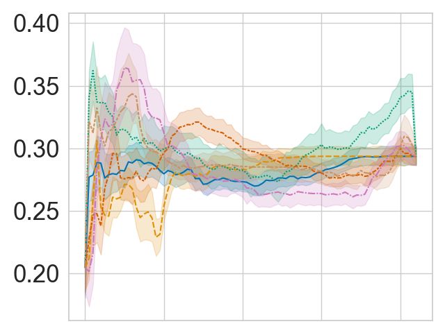
So far, most faithfulness comparisons of saliency maps focus on image classification tasks. There
is little work on computationally evaluating saliency maps in different tasks like Reinforcement
Learning. Furthermore, these evaluations often try to cover as many different saliency map approaches
as possible. This mostly leads to selections of algorithms with distinct motivations and requirements,
which is less helpful for people with specific requirements. Without full access to the agent’s inner
architecture, for example, one cannot use methods that rely on the inner workings of the agent but
must rely on model agnostic methods, which can be applied to any agent. Model agnostic saliency
maps mostly come in the form of perturbation-based approaches that perturb parts of the input and
observe how much this affects the agent’s decision.
This work presents a computational comparison of four perturbation-based saliency map approaches:
the original Occlusion Sensitivity approach [Zeiler and Fergus, 2014], Local Interpretable Model-
agnostic Explanations (LIME) [Ribeiro et al., 2016], a Noise Sensitivity approach proposed for DRL
[Greydanus et al., 2018], and Randomized Input Sampling for Explanation (RISE) [Petsiuk et al.,
2018]. As test-bed, we use four DRL agents trained on different Atari 2600 games. As metrics, we
use the sanity checks proposed by Adebayo et al. [2018], an insertion metric that slowly inserts the
most important pixels according to the saliency maps, and run-time analysis. As far as we know, this
is the first time that sanity checks were done for perturbation-based saliency maps and the first direct
comparison of how faithful different perturbation-based saliency maps are to DRL agents.

2   Related Work

The XAI literature is rapidly growing in recent years. In this work, we focus on saliency maps
that highlight the areas of the input which were important for the agents’ decision. There are three
main ideas on how to create saliency maps. The first idea is to use the gradient with respect to each
input to see how much small changes of this input influence the prediction [Simonyan et al., 2014,
Sundararajan et al., 2017, Selvaraju et al., 2020]. These approaches require the underlying agent to
be differentiable and need access to the gradients of the agent. The second group of methods uses
modified propagation rules to calculate how relevant each neuron of the network was, based on the
intermediate results of the prediction. Examples for this are Layer-wise Relevance Propagation (LRP)
[Bach et al., 2015] or PatternAttribution [Kindermans et al., 2018]. This idea requires access to the
inner workings of the agent. Finally, perturbation-based approaches perturb areas of the input and
measure how much this changes the output of the agent. The major advantage of perturbation-based
approaches over the aforementioned methods is their model agnosticism. Since they only use the in-
and outputs of the agent, they can be applied to any agent without adjustments.
The evaluation metrics for XAI approaches can be separated into two broad categories: human user
studies and computational measurements [Mohseni et al., 2020]. Examples of human user-studies
of saliency maps for DRL agents are Huber et al. [2020] and Anderson et al. [2019], who evaluate
LRP and Noise Sensitivity saliency maps respectively, with regards to mental models, trust, and
user satisfaction. To obtain more objective quantitative data it is important to additionally evaluate
explanations through computational measurements. Such measurements also provide an easy way to
collect preliminary data before recruiting users for a user study.
The most common computational measurement for saliency maps is input degradation. Here, the
input of the agent is gradually deleted, starting with the most relevant input features according to
the saliency map. In each step, the agent’s confidence is measured. If the saliency maps faithfully
describe the agent’s reasoning, then the agent’s confidence should fall quickly. For visual input, this
is either done by deleting individual pixels per step [Petsiuk et al., 2018, Ancona et al., 2018] or by
deleting patches of the image in each step [Samek et al., 2017, Kindermans et al., 2018, Schulz et al.,
2020]. In addition to deleting features, some newer approaches also propose an insertion metric where
they start with "empty" inputs and gradually insert input features [Ancona et al., 2018, Petsiuk et al.,
2018, Schulz et al., 2020]. The aforementioned image degradation tests mostly compared several
gradient-based methods and one or two perturbation-based and modified propagation approaches.
Furthermore, all previous tests use image classification tasks for their degradation measurements. As
far as we know, there are no input degradation benchmarks for Reinforcement Learning tasks.
Another computational measurement for saliency maps are the so-called sanity checks proposed
by Adebayo et al. [2018]. These tests measure whether the saliency map is dependent on what the
agent learned. One method for this is gradually randomizing the layers of the neural network and

                                                   2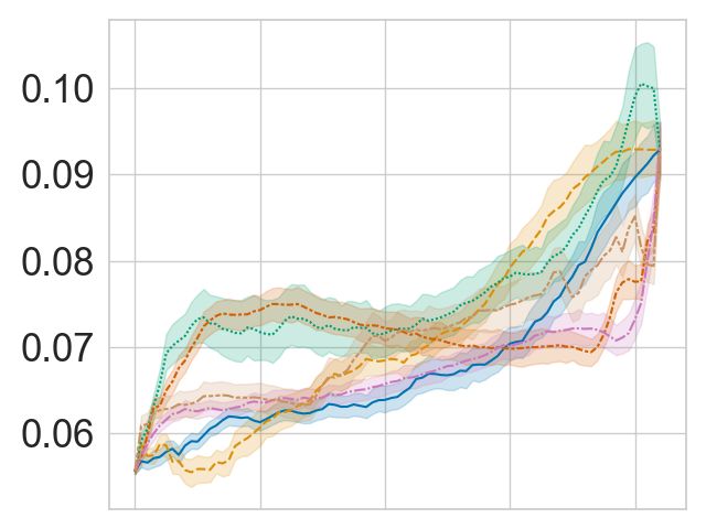
measuring how much this changes the saliency maps. Adebayo et al. did this for various gradient-
based approaches and Sixt et al. [2019] additionally tested LRP methods. As far as we know, there is
no work that computed sanity checks for perturbation-based saliency maps even though this is one of
the most popular saliency maps approaches.

3       Experiments
This section presents details about the implementation of our experiments. The code for all experi-
ments is available online.1
The test-bed in our paper is the Atari Learning Environment [Bellemare et al., 2013]. Four DRL
agents were trained on the games MsPacman (simplified to Pac-Man in this work), Space Invaders,
Frostbite, and Breakout using the Deep Q-Network (DQN) [Mnih et al., 2015] implementation of the
OpenAI Baselines Framework [Dhariwal et al., 2017] (available under the MIT License). We chose
the DQN because it is the most basic DRL architecture which most other DRL agents build upon.
The games were selected because the DQN performs very well on Breakout and Space Invaders but
performs badly on Frostbite and Pac-Man. The agents make predictions by observing the last 4 frames
of the game and then choose from a pool of possible actions. Hereby, each frame is down-sampled
and greyscaled resulting in 84 × 84 × 4 input images. The reward is given by the change in in-game
score since the last state, which we scaled such that the minimal possible reward is 1. To normalize
the output values between different inputs, we use a softmax activation function for the output layer.
Saliency Map Methods: The basic saliency map generation process is the same between all four
approaches compared in this work. Let f be the agent that takes a visual input I and maps it to a
confidence value for each possible action. Without loss of generality, f (I) describes the confidence in
the agent’s original prediction. That is the action which the agent chooses for the unperturbed image.
An input image I with height H and width W can be defined as a mapping I : ΛI → Rc of each pixel
λ ∈ ΛI = {1, ..., H} × {1, ..., W } to c channels (e.g. c = 4 for the Atari environment). To determine
the relevance of each pixel λ for the prediction of the agent, all four approaches feed perturbed
versions of I to the agent and then compare the resulting confidence values with the original results.
However, the approaches widely differ in the way the image is perturbed and how the relevance per
pixel is computed:
Occlusion Sensitivity [Zeiler and Fergus, 2014]: This approach creates perturbed images I 0 by
shifting a n × n patch across the original image I and occluding this patch by setting all the pixels
within to a certain color (e.g., black or gray). The importance S(λ) of each pixel λ inside the patch is
then computed based on the agents’ confidence after the perturbation
                                            S(λ) = 1 − f (I 0 ).                                    (1)
Since the original source does not go into details about the algorithm, we use the tf-explain implemen-
tation as reference [tf explain, 2019]. As long as the saliency maps are normalized this is equivalent
to f (I) − f (I 0 ), since all values in the saliency map are shifted by the same constant f (I) − 1.
Noise Sensitivity [Greydanus et al., 2018]: Instead of completely occluding patches of the image,
this approach adds noise to the image I by applying a Gaussian blur to a circle with radius r around a
pixel λ. The modified image I 0 (λ) is then used to compute the importance of the covered circle by
comparing the agent’s logit units π(x) (i.e., the outputs of all output neurons before softmax):
                                              1
                                    S(λ) =      ||π(I) − π(I 0 (λ))||2                              (2)
                                              2
This is done for every rth pixel, resulting in a temporary saliency map that is smaller than the input.
For the final saliency map, the result is up-sampled using bilinear interpolation.
RISE [Petsiuk et al., 2018]: This approach uses a set of N randomly generated masks {M1 , ..., MN }
for perturbation. To this end, temporary n × n masks are created by setting each element to 1 with a
probability p and 0 otherwise. These temporary masks are upsampled to the size of the input image
using bilinear interpolation. The images are perturbed by element-wise multiplication with those
masks I Mi . The relevance of each pixel λ is given by
                                                  N
                                             1 X
                                S(λI ) =             f (I   Mi ) · Mi (λ),                          (3)
                                           p · N i=1
    1
        https://github.com/belimmer/PerturbationSaliencyEvaluation

                                                     3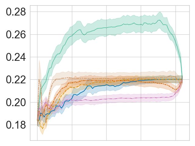
where Mi (λ) denotes the value of the pixel λ in the ith mask.
LIME [Ribeiro et al., 2016]: The original image is divided into superpixels using segmentation
algorithms. Perturbed variations of the image are generated by “deleting” different combinations of
superpixels (i.e., setting all pixels of the superpixels to 0). The combination of occluded images and
the corresponding predictions by the agent are then used to train a locally weighted interpretable
model for N steps. Analyzing the weights of this local model provides a relevance value for each
superpixel.
We evaluate the generated saliency maps using three different computational metrics:
Sanity Checks: The parameter randomization test proposed by Adebayo et al. [2018] measures the
dependence between the saliency maps and the parameters learned by the neural network of the agent.
To this end, the parameters of each layer in the network are randomized in a cascading manner, starting
with the output layer. Every time a new layer is randomized, a saliency map for this version of the
agent is created. The resulting saliency maps are then compared to the saliency map for the original
network, using three different similarity metrics (Spearman rank correlation, Structural Similarity
(SSIM), and Pearson correlation of the Histogram of Oriented Gradients (HOGs)). Following Sixt et al.
[2019], we account for saliency maps that differ only in sign by additionally computing similarity with
an inverse version of the saliency maps and using the maximum similarity. Analogous to Adebayo
et al. [2018] we tuned the similarity metrics such that two randomly sampled saliency maps with
uniform distribution have mean similarity values (0.0087, 0.0136, 0.0096) and two random saliency
maps with Gaussian distribution have mean similarity (0.0093, 0.0374, 0.0087). If the saliency maps
depend on the learned parameters of the agent then the saliency maps for the randomized model
should vastly differ from the ones of the original model.
Insertion Metric: To test the premise that the most relevant pixels, according to the saliency maps,
have the highest impact on the agent, we use the insertion metric proposed by Petsiuk et al. [2018].
We do not use a deletion metric, since we feel that it is too similar to the way that perturbation-based
saliency maps are created. The insertion metric starts with a fully occluded image (i.e. the values
of all pixels are set to 0). In each step, 84 occluded pixels (approx. 1.2% of the full image) are
uncovered, starting with the most relevant pixels according to the saliency map. For LIME, the
superpixels are sorted by their relevance but the order of pixels within superpixels is randomized. The
partly uncovered image is then fed to the agent and its confidence in the original prediction, which the
agent chooses for the full image, is stored. If the saliency map correctly highlights the most important
pixels, then the agent’s confidence should increase quickly for each partly uncovered image.
Run-time Analysis: The run-time of an algorithm can be an important aspect when choosing between
different approaches. Therefore, we computed the mean time it took each algorithm to create a single
saliency map using the timeit python library. To this end, we measured a total of 1000 saliency maps
for each game.
Hardware: All the insertion metric and run-time tests were done on the same machine with an
Nvidia GeForce GTX TITAN X GPU to ensure comparability of the run-time results. The sanity
checks and parameter tests were divided between the aforementioned machine and another one with
an Nvidia GeForce GTX 1080 Ti GPU.

4   Parameter Tuning

All the perturbation-based saliency map approaches tested in this work depend on a choice of
parameters. To get an estimate of which parameters work well with the Atari environment, we
tested a range of different parameters for each approach. Since LIME and RISE in particular have
long computation times and a large number of possible parameter combinations we only used 5
images to test the parameters. We chose the images among a stream of Pac-Man game-play with
the HIGHLIGHTS-DIV algorithm which selects a diverse set of states that give a good overview of
the agent’s policy [Amir and Amir, 2018]. These states were shown to produce more informative
saliency maps for human observers than randomly sampled states [Huber et al., 2020]. While the
sample size is too small to find optimal parameters, this does allow us to get a good estimate of the
approaches’ performance for a wide range of different parameters in a reasonable amount of time.
However, the process still took up to 10 hours for some of the segmentation algorithms we tested
with LIME. As Metric we used the Insertion Metric to estimate how well the generated saliency maps
capture the agent’s reasoning.

                                                   4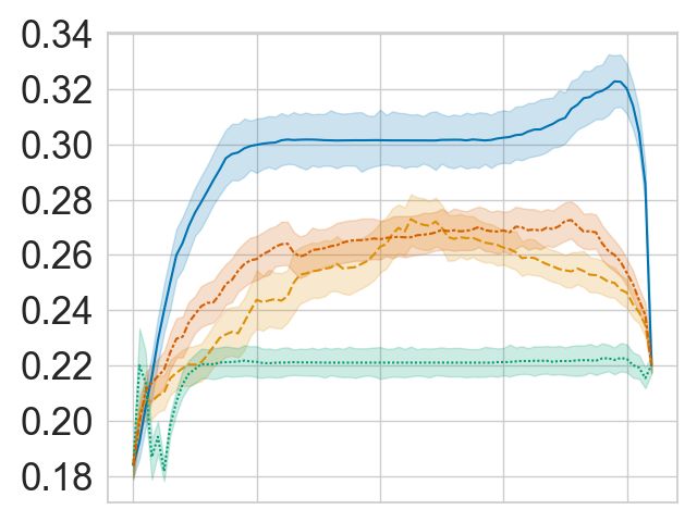
Input State Occlusion     RISE         NS           NS Black NS Chosen LIME              LIME
                Sensitivity              Original                 Action Quickshift          SLIC

Figure 1: Example saliency maps for three different Pac-Man game states generated by each of the
approaches investigated in this paper (NS is Noise Sensitivity). The circles mark Pac-Man’s position.
For the LIME variants we only show the top 5 superpixels as is custom with this approach.

For Occlusion Sensitivity, we tested patches of size 1 to 10 and two different occlusion colors: black
and gray. Independent of the size, black was better than gray. For Noise Sensitivity, we tested circles
with a radius of 1 to 10. In general, the smaller the patch size and radius, the better were the results,
while the run-time increased. Since LIME and RISE are not suited to create such fine-granular
saliency maps, we decided against using the sizes 1 or 2. Moreover, the results of sizes 3 and 4 were
very close and 4 even beat 3. Therefore, we decided to use patch size and radius 4 such that the
results are more comparable with the other approaches.
For RISE we tested 500, 1000,...,3000 masks of size 4 to 24. The probability p with which each pixel
is occluded varied between 0.1 and 0.9 in steps of 0.1. The best parameters were a probability of 0.8,
mask size 18, and 3000 masks.
For LIME we tested the three most common Segmentation techniques SLIC, Quickshift and Felzen-
szwalb and varied the number of samples on which the local interpretable model is trained. For the
number of learning steps we took the default number of samples (1000) and increased it in steps
of 500 up to 3000. This range produced good results (all top 5 results contain some parameter
combinations with less than 3000 samples) while the run-time per saliency map did not diverge too
much from the other approaches. To determine which parameter ranges we should use for each
segmentation algorithm, we performed preliminary tests where we visually checked which parameters
resulted in different segmentation. The exact parameters we used are listed in Appendix A.1. The best
parameters for Felzenszwalb were scale factor 1, Gaussian smoothing kernel width 0.25, minimum
component size 2 and 2500 training samples. The best parameters for SLIC were 80 segments,
compactness factor 10, Gaussian smoothing kernel width 0.5, and 1000 samples. Quickshift obtained
the best result with kernel size 1, max distance 4, color ratio 0 and 3000 samples.
The top five results of all approaches and segmentation algorithms can be seen in Appendix A.1 and
the full results can be seen in our GitHub Repository.2

5        Results
Visual Assessment: Fig. 1 shows example saliency maps for the Pac-Man agent (saliency maps
for the remaining agents are shown in Appendix A.2). We only show the two LIME segmentation
algorithms that performed better on Pac-Man. To prevent cherry-picking, the states were chosen by
the HIGHLIGHTS-DIV algorithm which selects diverse and informative states about the agent’s
strategy [Amir and Amir, 2018]. Except for the Noise Sensitivity approaches with blurring, the
saliency maps generally seem to highlight Pac-Man and its surroundings.
Sanity Checks: The results of the parameter randomization test are shown in Fig. 2. The lower the
scores the higher the dependence on the agents’ learned parameters. Fig. 3 shows an example for
the different saliency maps during a single run of the sanity check. Notably, LIME has a very high
     2
         https://github.com/belimmer/PerturbationSaliencyEvaluation

                                                    5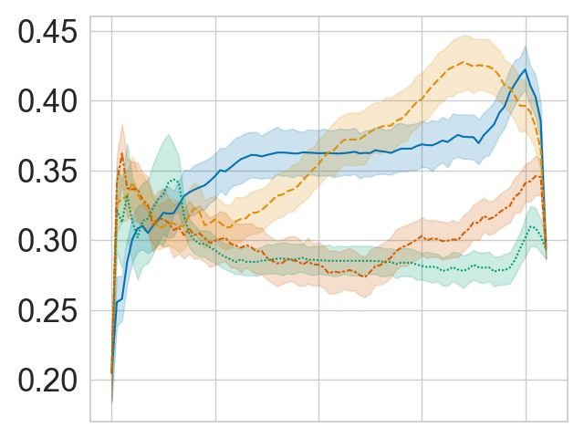
1.0
 0.8
 0.6
 0.4
 0.2
 0.0
                Spearman                          SSIM                            Pearson
Figure 2: Results of the parameter randomization sanity check for the different saliency map
approaches. Measured for 1000 states of each of the 4 tested games. Starting from the left, each mark
represents an additional randomized layer starting with the output layer. The y-axis shows the average
similarity values (Spearman rank correlation, SSIM, Pearson correlation of the HOGs). High values
indicate a low parameter dependence. Since all LIME variants were similar, we only show the one
with the highest parameter dependence (Quickshift). The translucent error bands show the 99% CI.

  Occlusion      RISE         NS       NS Black NS Chosen LIME                LIME        LIME
                            Original             Action Quickshift            SLIC     Felzenszwalb

Figure 3: Example saliency maps for the parameter randomization sanity check. All saliency maps
are generated for the first state in Fig. 1. From top to bottom each row after the first is generated for
agents with cascadingly randomized layers starting with the output layer. In contrast to Fig. 1, the
LIME saliency maps show all superpixels with their corresponding importance values.

Pearson correlation of HOGs, and RISE’s similarity values increase with the number of randomized
layers. Furthermore, the original Noise Sensitivity has very low dependence on the parameters of the
output layer when compared to Occlusion Sensitivity. Since those two approaches are very similar
in theory, we implemented two modifications of Noise Sensitivity to investigate the reason for this
difference in parameter dependence. First, Noise Sensitivity Black occludes the circles in the Noise
Sensitivity approach with black color instead of blurring them. Second, Noise Sensitivity Chosen
Action changes the way that the importance of each pixel is calculated from Eq. (2), which takes all
actions into account, to the one used by Occlusion Sensitivity (Eq. (1)), which focuses on the chosen
action. We did not test a combination of black circles and the Occlusion Sensitivity importance
calculation, since that would be pretty much equivalent to Occlusion Sensitivity with circles instead
of squares. While the black occlusion did not really change the sanity check results, the change of
the importance calculation immensely increased the dependence on the learned parameters of the
output layer. Noise Sensitivity Chosen Action and Occlusion Sensitivity both show high parameter
dependence across all three similarity metrics.

                                                   6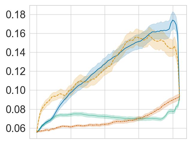
Figure 4: The insertion metric results for four different Atari games (from left to right: Pac-Man,
Space Invaders, Breakout, and Frostbite), averaged over 1000 steps. The x-axis shows the percentage
of inserted pixels and the y-axis shows the average confidence in the original prediction for those
modified states. For Noise Sensitivity and LIME we only plot the variant with the highest AUC. The
error bands show the 99% CI.

 AUC                      Pac-Man       Space Invaders Breakout          Frostbite
  Occlusion Sensitivity 0.351           0.293           0.354            0.123
  RISE                    0.351         0.248           0.359            0.123
 NS Original              0.130         0.211           0.281            0.068
 NS Black                 0.141         0.213           0.279            0.072
 NS Chosen Action         0.115         0.257           0.301            0.076
  LIME Quickshift         0.21          0.214           0.289            0.072
  LIME SLIC               0.197         0.202           0.285            0.067
  LIME Felzenszwalb 0.172               0.219           0.292            0.071
Table 1: The average Area Under the Curve (AUC) for the graphs obtained by the insertion metric
(Fig. 4). NS is Noise Sensitivity. The average was computed across 1000 states for each Atari model.

Insertion Metric: Fig. 4 shows the insertion metric results for the best parameters for each game
(the remaining LIME and Noise Sensitivity variants can be seen in Appendix A.2). Table 1 reports the
average Area Under the Curve (AUC) for all parameter combinations. Across all games, Occlusion
Sensitivity and RISE achieve the highest AUC values. LIME and Noise Sensitivity are less good.
Noticeably, the confidence often increases over the confidence for the full image. This is related to
the fact that the agents are not perfectly sure about their actions (average confidence around 0.3).
Furthermore, we use a softmax activation function which increases the confidence in the observed
action when the agents’ confidence in other actions decreases.
Run-time Analysis: The average run-times for each of the tested saliency map approaches with the
final parameters we used are shown in Table 2. Occlusion Sensitivity and Noise Sensitivity black,
which simply occlude image patches with black pixels, perform faster than the approaches with more
complex image perturbations. However, this strongly depends on the chosen parameters as can be
seen in the low run-time of LIME with SLIC segmentation. More time measurements from our
parameter tests can be seen in Appendix A.1.

6   Discussion
Occlusion Sensitivity performed the best across all tests we ran. It achieved the highest AUC values
in 3 out of 4 games and is only slightly behind the best approach in the remaining game (Fig. 4 and
Table 1). This result is in contrast to the evaluations by Schulz et al. [2020] and Petsiuk et al. [2018],
where Occlusion Sensitivity was among the worst of the tested approaches. We think that this is
mainly due to the differences in the domains. In most Atari games, a black square really means that

 Occlusion RISE NS             NS        NS Chosen LIME Quick- LIME               LIME Felzen-
 Sensitivity         Blur      Black Action            shift           Slic       szwalb
 0.722        4.914 1.614 0.712 1.632                  3.135           0.858      3.189
Table 2: The mean number of seconds it took an perturbation-based approach to generate one saliency
map. The average was computed across 1000 states for each game.

                                                    7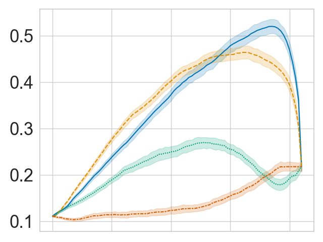
there is no relevant object at this position. This is not the case for the real-world images used by
Petsiuk et al. and Schulz et al.. Moreover, Schulz et al. use a different implementation of the insertion
metric, where n × n patches are inserted in each step instead of the top n pixels. Ancona et al.
[2018], who use individual pixels in each step, found that Occlusion Sensitivity performed similarly
to the compared gradient-based method. In the parameter randomization sanity checks, Occlusion
Sensitivity is very dependent on the learned parameters (Fig. 2). The parameter dependence is
among the highest of all the perturbation-based saliency maps we tested and it is on par with the best
gradient-based saliency maps tested by Adebayo et al. [2018]. However, their tests were done on
another domain so it should be taken with a grain of salt. Finally, Occlusion Sensitivity has one of
the lowest run-times (Table 2) and was the easiest for us to find suiting parameters.
Noise Sensitivity, in its original formulation, performed quite badly in our tests. It is especially
concerning, that the approach only showed very little dependence on the parameters of the output
layer (Fig. 2). Since the output layer has the highest impact on the actual decision of a network,
it is crucial that a faithful saliency map depends on the weights learned in this layer. Our results
empirically show that replacing the original equation to calculate the importance of each pixel S(I 0 )
(Eq. (2)) with the equation used by Occlusion Sensitivity (Eq. (1)) greatly increases the parameter
dependence. We think that this is due to the fact that Eq. (2) takes all actions into account and
therefore measures a general increase in entropy within the activations of the output layer. In contrast,
Eq. (1) only measures the action which is actually chosen and therefore captures a more specific
change in the output layer activation. Recently, Puri et al. [2020] also criticized that the saliency maps
by Greydanus et al. [2018] take all actions into account. The results of our sanity checks provide the
first computational evidence for this critique. Puri et al. propose a solution to this problem, which is
similar to our adjustment. In the future, we would like to include their approach in our evaluation.
Changing the perturbation within the circles from blurring to black occlusion did not have a big
impact on the parameter dependence. Interestingly, however, changing the perturbation in this way
increased the insertion metric score for the game Pac-Man (Table 1). For this game, Greydanus
et al. [2018] reported that their Noise Sensitivity approach produced unintuitive saliency maps. Our
results indicate that this is not due to a flaw in the agents but rather that blurred perturbation is not
suitable for this game. In the other games, the Noise Sensitivity Chosen Action variant achieves higher
insertion metric scores than the other Noise Sensitivity variants (Table 1). In Space Invaders, it even
obtained the second-highest AUC among all saliency approaches. Together with its good parameter
dependence and the fact that it was easy to find suiting parameters for this approach, we think that this
modified Noise Sensitivity is a good alternative to Occlusion Sensitivity for environments without a
single color that is suited to occlude the input.
RISE obtained comparable AUC values to Occlusion Sensitivity in the insertion metric (Fig. 4 and
Table 1). In Breakout it had the highest AUC but in Space Invaders it was below both Occlusion
and the Noise Sensitivity Chosen Action. These high scores are in line with the results by Petsiuk
et al. [2018] who found their RISE approach to perform better than Occlusion Sensitivity, LIME,
and a gradient-based method on an image classification task. Notably, RISE required a much higher
run-time to acquire those results (Table 2) and took more resources for fine-tuning than Occlusion and
Noise Sensitivity. Visually, the saliency maps produced by RISE and Occlusion Sensitivity mostly
agree on the most relevant region in the input states (see Fig. 1). However, RISE produces more noisy
saliency maps making it harder to quickly interpret the results. This noise might also be related to
the biggest disadvantage of RISE. During the parameter randomization sanity check, RISE saliency
maps got more similar to the original explanation after the first randomization of the output layer
(Fig. 2). Investigating further, we found that nearly all saliency maps, which are generated after more
than the output layer was randomized, look the same (Fig. 3). It seems like they reflect the structure
of the randomly generated masks. We made sure that the same masks are used for all saliency maps
during the sanity check. Since the background noise in the RISE saliency maps for the fully trained
agent also seems to reflect the structure of the masks, this noise might be the reason for the similarity.
Thus, the high similarity values might not stem from low parameter dependence. However, this needs
to be investigated further before the approach can be relied upon.
LIME was the hardest approach to fine-tune. General parameters, like the number of training samples
for the local model, combined with different segmentation algorithms that have their own parameters,
result in an exponentially growing amount of possible parameter combinations. Even when taking all
those parameters into account and trying to optimize for the insertion metric, we were not able to
achieve good results in this metric (Fig. 4 and Table 1). This contrasts the findings by Petsiuk et al.

                                                    8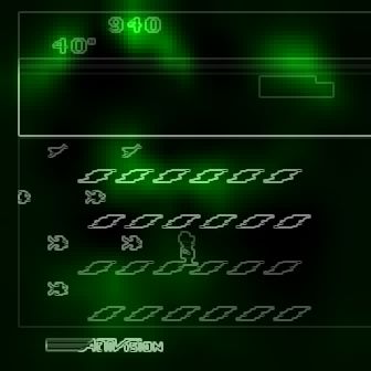
[2018] who found LIME to perform better than Occlusion Sensitivity in an image classification task.
Our results indicate that LIME is not suited to identify the most important pixels for Atari agents.
LIME’s run-time highly depends on the chosen parameters and we found that it could easily explode
during our parameter tests, making the parameter search even more resource-intensive (Appendix
A.1). However, the final parameters we used were faster than RISE. The SLIC segmentation variant
even was among the fastest saliency map approaches (Table 2). The main positive result for LIME is
its high dependence on the learned parameters of the agents. Here, the best LIME variant (Quickshift)
was on par with Occlusion Sensitivity and Noise Sensitivity Chosen Action. Only the Pearson
correlation of the HOGs was very high between LIME saliency maps for the trained and randomized
agents. However, the reason for this is not necessarily a low dependence on the agent’s learned
weights. More likely it is due to the fact that all LIME saliency maps for a given state work with
the same superpixels. Since every pixel inside a superpixel has the same value there are hard edges
between the superpixels. These edges are captured by the HOGs and result in high values of the
Pearson correlation of the HOGs.

Limitations As with every evaluation, our study has limitations. First, we did not fine-tune the
approaches for each game individually. To save time, we only used one game to find parameters
that work reasonably well with the general Atari environment. It is likely that there are differences
between the optimal parameters for each game. However, since the tuning process was the same for
all approaches, we think that the results are still representative. The results for a fully fine-tuned
game can be seen with Pac-Man. Second, the metrics in our evaluation only provide an estimate of
the faithfulness of saliency maps. Especially the insertion metric is only an approximation of how
well a saliency map captures the reasoning of an agent. So far, there is no way to obtain perfect
ground truth about which pixels were the most important for a DRL agent. In this context, we want
to emphasize that we do not claim that the best saliency maps according to our evaluation perfectly
capture the agents’ reasoning. Creating such perfect saliency maps is still an open challenge and this
work aims to guide the development in this direction. Solely relying on saliency maps to be 100%
accurate in high-risk domains like healthcare could lead to a negative social impact. For now, saliency
maps should not be used in isolation but as part of an interpretability toolbox. Finally, we chose one
of the most basic DRL architectures without any sophisticated adjustments for our experiments to
ensure that the results generalize as much as possible. Since all the saliency map approaches we
tested are model-agnostic the results should not change drastically with different agent architectures.
In particular, we expect the sanity check results to be very independent of the underlying agents.
However, to be absolutely sure, we plan to include other architectures in future experiments.

7   Conclusion

This paper compared four different perturbation-based saliency map approaches measuring their
dependence on the agent’s parameters, their faithfulness to the agent’s reasoning, and their run-time.
The three most interesting findings from our experiments are:

       • The simplest approach produces the best-suited saliency map for our agents. Occlusion
         Sensitivity with black occlusion color performs the best across all our metrics.
       • Noise Sensitivity, which was proposed for the Atari environment and is one of the most
         prominent saliency map methods for DRL agents, did not perform well in our tests and
         should be adjusted in the future. Especially concerning is the fact that the original Noise
         sensitivity approach shows little dependence on the learned parameters of the output layer.
         We empirically show that replacing the original importance calculation with the one used by
         Occlusion Sensitivity, which only takes the chosen action into account, drastically increases
         parameter dependence. Moreover, it also improves the insertion metric results in most games
         we tested. Thus, we propose that this variant should be used in the future.
       • Both LIME and RISE showed more severe issues in our tests. Even with extensive parameter
         tuning to optimize the insertion metric we did not manage to achieve good insertion metric
         results with LIME. In contrast, RISE failed the parameter randomization sanity check by
         showing high similarities between saliency maps for trained and randomized agents. While
         we think that this might not completely stem from low parameter dependence, it should be
         investigated further before the approach can be relied upon.

                                                  9
The computational measurements in this work present a first step to fully evaluate perturbation-based
saliency maps for DRL. In the future, we want to build upon the insights from this paper and conduct
a human user-study , similar to the one we did in Huber et al. [2020], to evaluate how useful the
saliency map approaches with good computational results are for actual end-users.
References
J. Adebayo, J. Gilmer, M. Muelly, I. Goodfellow, M. Hardt, and B. Kim. Sanity checks for saliency
maps. In Advances in Neural Information Processing Systems, pages 9505–9515, 2018.
D. Amir and O. Amir. HIGHLIGHTS: summarizing agent behavior to people. In Proceedings of the
17th International Conference on Autonomous Agents and MultiAgent Systems, pages 1168–1176,
2018. URL http://dl.acm.org/citation.cfm?id=3237869.
M. Ancona, E. Ceolini, C. Öztireli, and M. Gross. Towards better understanding of gradient-based
attribution methods for deep neural networks. In 6th International Conference on Learning
Representations, 2018. URL https://openreview.net/forum?id=Sy21R9JAW.
A. Anderson, J. Dodge, A. Sadarangani, Z. Juozapaitis, E. Newman, J. Irvine, S. Chattopadhyay,
A. Fern, and M. Burnett. Explaining reinforcement learning to mere mortals: An empirical study. In
Proceedings of the Twenty-Eighth International Joint Conference on Artificial Intelligence, IJCAI-
19, pages 1328–1334. International Joint Conferences on Artificial Intelligence Organization, 7
2019. URL https://doi.org/10.24963/ijcai.2019/184.
A. B. Arrieta, N. D. Rodríguez, J. D. Ser, A. Bennetot, S. Tabik, A. Barbado, S. García, S. Gil-Lopez,
D. Molina, R. Benjamins, R. Chatila, and F. Herrera. Explainable artificial intelligence (XAI):
concepts, taxonomies, opportunities and challenges toward responsible AI. Inf. Fusion, 58:82–115,
2020. doi: 10.1016/j.inffus.2019.12.012.
S. Bach, A. Binder, G. Montavon, F. Klauschen, K.-R. Müller, and W. Samek. On pixel-wise
explanations for non-linear classifier decisions by layer-wise relevance propagation. PloS one, 10
(7), 2015.
M. G. Bellemare, Y. Naddaf, J. Veness, and M. Bowling. The arcade learning environment: An
evaluation platform for general agents. J. Artif. Intell. Res., 47:253–279, 2013. doi: 10.1613/jair.
3912. URL https://doi.org/10.1613/jair.3912.
P. Dhariwal, C. Hesse, O. Klimov, A. Nichol, M. Plappert, A. Radford, J. Schulman, S. Sidor, Y. Wu,
and P. Zhokhov. Openai baselines. https://github.com/openai/baselines, 2017.
S. Greydanus, A. Koul, J. Dodge, and A. Fern. Visualizing and understanding atari agents. In
Proceedings of the 35th International Conference on Machine Learning, pages 1787–1796, 2018.
URL http://proceedings.mlr.press/v80/greydanus18a.html.
T. Huber, K. Weitz, E. André, and O. Amir. Local and global explanations of agent behavior:
Integrating strategy summaries with saliency maps. CoRR, abs/2005.08874, 2020. URL https:
//arxiv.org/abs/2005.08874.
P. Kindermans, K. T. Schütt, M. Alber, K. Müller, D. Erhan, B. Kim, and S. Dähne. Learning how
to explain neural networks: Patternnet and patternattribution. In 6th International Conference
on Learning Representations. OpenReview.net, 2018. URL https://openreview.net/forum?
id=Hkn7CBaTW.
V. Mnih, K. Kavukcuoglu, D. Silver, A. A. Rusu, J. Veness, M. G. Bellemare, A. Graves, M. Ried-
miller, A. K. Fidjeland, G. Ostrovski, et al. Human-level control through deep reinforcement
learning. nature, 518(7540):529–533, 2015.
S. Mohseni, N. Zarei, and E. D. Ragan. A multidisciplinary survey and framework for design and
evaluation of explainable ai systems, 2020.
V. Petsiuk, A. Das, and K. Saenko. Rise: Randomized input sampling for explanation of black-box
models. arXiv preprint arXiv:1806.07421, 2018.
10N. Puri, S. Verma, P. Gupta, D. Kayastha, S. Deshmukh, B. Krishnamurthy, and S. Singh. Explain
your move: Understanding agent actions using specific and relevant feature attribution. In 8th
International Conference on Learning Representations, ICLR. OpenReview.net, 2020.
M. T. Ribeiro, S. Singh, and C. Guestrin. "Why should i trust you?" Explaining the predictions of
any classifier. In Proceedings of the 22nd ACM SIGKDD international conference on knowledge
discovery and data mining, pages 1135–1144, 2016.
W. Samek, A. Binder, G. Montavon, S. Lapuschkin, and K. Müller. Evaluating the visualization
of what a deep neural network has learned. IEEE Trans. Neural Networks Learn. Syst., 28(11):
2660–2673, 2017. URL https://doi.org/10.1109/TNNLS.2016.2599820.
K. Schulz, L. Sixt, F. Tombari, and T. Landgraf. Restricting the flow: Information bottlenecks for
attribution. In 8th International Conference on Learning Representations, 2020. URL https:
//openreview.net/forum?id=S1xWh1rYwB.
A. D. Selbst and S. Barocas. The intuitive appeal of explainable machines. Fordham L. Rev., 87:1085,
2018.
R. R. Selvaraju, M. Cogswell, A. Das, R. Vedantam, D. Parikh, and D. Batra. Grad-CAM: Visual
explanations from deep networks via gradient-based localization. Int. J. Comput. Vis., 128(2):
336–359, 2020. URL https://doi.org/10.1007/s11263-019-01228-7.
K. Simonyan, A. Vedaldi, and A. Zisserman. Deep inside convolutional networks: Visualising
image classification models and saliency maps. In 2nd International Conference on Learning
Representations, 2014. URL http://arxiv.org/abs/1312.6034.
L. Sixt, M. Granz, and T. Landgraf. When explanations lie: Why modified BP attribution fails. CoRR,
abs/1912.09818, 2019. URL http://arxiv.org/abs/1912.09818.
P. Stone, R. Brooks, E. Brynjolfsson, R. Calo, O. Etzioni, G. Hager, J. Hirschberg, S. Kalyanakrishnan,
E. Kamar, S. Kraus, K. Leyton-Brown, D. Parkes, P. William, S. AnnaLee, S. Julie, T. Milind, and
T. Astro. Artificial intelligence and life in 2030. One Hundred Year Study on Artificial Intelligence:
Report of the 2015-2016 Study Panel, 2016.
M. Sundararajan, A. Taly, and Q. Yan. Axiomatic attribution for deep networks. In D. Precup
and Y. W. Teh, editors, Proceedings of the 34th International Conference on Machine Learning,
volume 70 of Proceedings of Machine Learning Research, pages 3319–3328. PMLR, 2017. URL
http://proceedings.mlr.press/v70/sundararajan17a.html.
tf explain. Interpretability methods for tf.keras models with tensorflow 2.0. https://github.com/
sicara/tf-explain, 2019.
M. D. Zeiler and R. Fergus. Visualizing and understanding convolutional networks. In European
conference on computer vision, pages 818–833. Springer, 2014.
11A Appendix
A.1 Parameter Tuning Results
Table 3, 4, and 5 show the top five results of the parameter tests, as described in Section 4 of the main
paper, for Occlusion Sensitivity, Noise Sensitivity, and RISE, respectively. Note that the run-time
values in the appendix might differ from the ones in the main results since we ran some of the
parameter tests on a different machine than the run-time tests.
AUC Patch Size Color Time AUC Radius Time
4.513 1 0.0 64.622 0.992 1 127.870
4.020 2 0.0 14.593 0.917 2 34.349
3.160 4 0.0 3.958 0.858 5 5.864
3.130 3 0.0 7.274 0.854 4 8.060
2.682 5 0.0 2.517 0.852 3 14.868
Table 3: Best parameters for Occlusion Sensitivity. Table 4: Best parameters for Noise Sensitivity.
AUC Propability p Mask Size Number of Masks Time
3.288 0.8 18 3000 25.928
3.207 0.8 22 3000 25.374
3.184 0.8 21 2500 21.091
3.182 0.7 24 3000 26.170
3.145 0.8 16 3000 25.351
Table 5: Best parameters for RISE
For LIME we tested the three most prominent segmentation algorithms: Felzenszwalb, SLIC, and
Quickshift. For Felzenszwalb segmentation we used a scale factor of 1,21,...,101, a minimum
component size from 1 to 8 and Gaussian smoothing kernels with width σ of 0,0.25,...,1. The top
results are shown in Table 6. For SLIC we tested 40,60 to 240 segments, a compactness factor of
0.001,0.01,...,10 and Gaussian smoothing kernels with width σ of 0,0.25,...,1. The top five parameter
combinations can be seen in Table 7. Finally, we tested Quickshift with a color ratio of 0.0,0.33,0.66
and 0.99, a kernel size from 1 to 6 and a max distance of kernelsize ∗ i, where i goes from 1 to 4.
The top results are shown in Table 8.
AUC Scale Sigma Minimum Size Num Samples Time
1.843 1 0.25 2 2500 7.116
1.792 1 1.0 2 3000 21.70
1.741 1 1.0 0 3000 53.359
1.740 1 1.0 1 1000 17.367
1.731 1 0.25 1 1000 5.528
Table 6: Best parameters for LIME with Felzenszwalb segmentation.
12AUC Number of Segments Compactness Sigma Num Samples Time
1.987 80 10.0 0.5 1000 0.835
1.966 80 10.0 0.5 3000 2.429
1.952 80 10.0 0.75 1000 0.859
1.949 80 10.0 0.5 1500 1.256
1.942 80 10.0 0.25 2500 2.132
Table 7: Best parameters for LIME with SLIC segmentation.
AUC Kernel Size Max Distance Ratio Num Samples Time
2.061 1 4 0.0 3000 2.957
2.051 1 1 0.33 3000 13.380
2.014 1 4 0.0 2500 2.687
2.005 1 1 0.66 3000 13.086
1.951 1 1 0.99 2500 10.911
Table 8: Best parameters for LIME with Quickshift segmentation.
13A.2 Additional Results
In this section, we show some additional results that did not fit in the main paper. Fig. 5 shows
example saliency maps for HIGHLIGHT-DIV states of the remaining three games apart from Pac-
Man. Fig. 6 shows the results of the sanity checks for LIME with all three segmentation algorithms.
The insertion metric results for all variants of Noise Sensitivity and LIME are shown in Fig. 7.
Input State Occlusion RISE NS NS Black NS Chosen LIME LIME
Sensitivity Original Action Quickshift Felzens.
Figure 5: Example saliency maps for the remaining games we tested. From top to bottom: Breakout,
Space Invaders and Frostbite. NS is Noise Sensitivity. For the LIME variants we only show the top 5
superpixels as is custom with this approach and we only show the two segmentation variants that
performed the best on these games.
1.0
0.8
0.6
0.4
0.2
0.0
Spearman SSIM Pearson
Figure 6: Results of the parameter randomization sanity check for the different LIME segmentation
variants. Measured for 1000 states of each of the 4 tested games. Starting from the left, each mark
represents an additional randomized layer starting with the output layer. The y-axis shows the average
similarity values (Spearman rank correlation, SSIM, Pearson correlation of the HOGs). High values
indicate a low parameter dependence. The translucent error bands show the 99% CI.
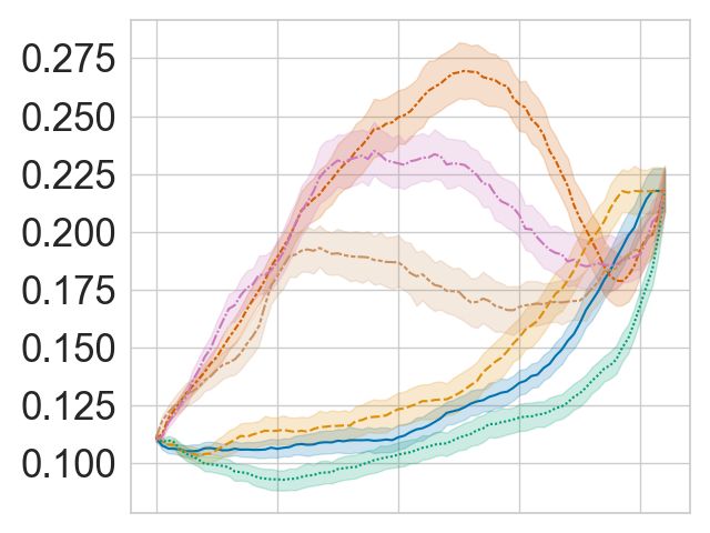
14Pac-Man Space Invaders
Breakout Frostbite
Figure 7: The remaining insertion metric results for four different Atari games, averaged over 1000
steps. NS is Noise Sensitivity. The x-axis shows the percentage of inserted pixels and the y-axis
shows the average confidence in the original prediction for those modified states. The error bands
show the 99% CI.
15You can also read