QCMC: Quasi-conformal Parameterizations for Multiply-connected domains
←
→
Page content transcription
If your browser does not render page correctly, please read the page content below
Noname manuscript No.
(will be inserted by the editor)

QCMC: Quasi-conformal Parameterizations for Multiply-connected
domains

Kin Tat Ho · Lok Ming Lui

Received: date / Accepted: date

Abstract This paper presents a method to compute the quasi-conformal parameterization (QCMC)
for a multiply-connected 2D domain or surface. QCMC computes a quasi-conformal map from a
multiply-connected domain S onto a punctured disk DS associated with a given Beltrami differential.
The Beltrami differential, which measures the conformality distortion, is a complex-valued function
µ : S → C with supremum norm strictly less than 1. Every Beltrami differential gives a conformal
structure of S. Hence, the conformal module of DS , which are the radii and centers of the inner
circles, can be fully determined by µ, up to a Möbius transformation. In this paper, we propose an
iterative algorithm to simultaneously search for the conformal module and the optimal quasi-conformal
parameterization. The key idea is to minimize the Beltrami energy with the conformal module of the
parameter domain incorporated. The optimal solution is our desired quasi-conformal parameterization
onto a punctured disk. The parameterization of the multiply-connected domain simplifies numerical
computations and has important applications in various fields, such as in computer graphics and
visions. Experiments have been carried out on synthetic data together with real multiply-connected
Riemann surfaces. Results show that our proposed method can efficiently compute quasi-conformal
parameterizations of multiply-connected domains and outperforms other state-of-the-art algorithms.
Applications of the proposed parameterization technique have also been explored.
Keywords Quasi-conformal · parameterization · multiply-connected · Beltrami differential ·
conformal module · Beltrami energy
Mathematics Subject Classification (2000) 37K25 · 68U05 · 68U10

1 Introduction

Parameterization refers to the process of mapping a complicated domain one-to-one and onto a simple
canonical domain. For example, according to the Riemann mapping theorem, a simply-connected open
surface can be conformally mapped onto the unit disk D. The geometry of the canonical domain is
usually much simpler than its original domain. Hence, by parameterizing a complicated domain onto
its simple parameter domain, a lot of numerical computations can be simplified.
    Parameterizations have been extensively studied and various parameterization algorithms have
been developed. In particular, conformal parameterizations have been widely used, since it preserves
the local geometry well. For example, in computer graphics, conformal parameterizations of 3D sur-
faces onto 2D images have been applied for texture mapping [2]. While in medical imaging, conformal
parameterizations have been used for obtaining surface registration between various anatomical struc-
tures, such as the brain cortical surfaces [9, 10, 16]. Conformal parameterizations have also been applied
to solve PDEs on complicated 2D domains or surfaces [31][40][41].
K.T. Ho
Dept. of Mathematics, Chinese University of Hong Kong
E-mail: ktho@math.cuhk.edu.hk
L.M. Lui
Dept. of Mathematics, Chinese University of Hong Kong
E-mail: lmlui@math.cuhk.edu.hk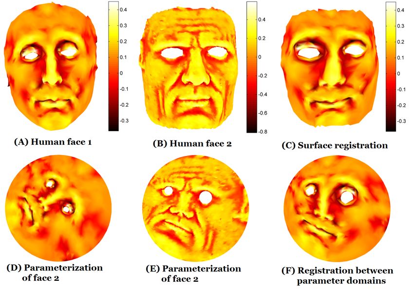
2                                                                               Kin Tat Ho, Lok Ming Lui

     In case of extra constraints have to be enforced, obtaining conformal surface parameterizations may
not be feasible. In such situations, quasi-conformal parameterizations, which allow bounded amount of
conformality distortions, have to be considered. The conformality distortion can be measured by Bel-
trami differential. Quasi-conformal parameterization of a complicated domain onto a simple parameter
domain is useful and have found important applications in various fields. For example, in computer
graphics, constrained texture mapping that matches feature landmarks are quasi-conformal param-
eterizations [26]. Besides, by parameterizing two surfaces quasi-conformally onto simple parameter
domains in R2 , Quasi-conformal map between two Riemann surfaces with a given Beltrami differential
can be easily computed. Quasi-conformal parameterization can also simplify the process of solving the
elliptic partial differential equations (PDEs) on a complicated surface. Elliptic PDEs arise in many
imaging problems, such as in surface registration. Through quasi-conformal parameterization, the el-
liptic PDE on a complicated domain can be formulated into a simpler PDE on the simple parameter
domain. For instance, the elliptic PDE ∇ · (A∇f ) = g on a multiply-connected surface S with certain
boundary conditions can be converted to a simpler PDE: ∆f ◦ φ = g ◦ φ on a circle domain, where φ is
the quasi-conformal parameterization of S whose Beltrami differential is given by A (SPD matrix). The
simpler PDE defined on a simpler parameter domain can be solved much easier. Other applications of
quasi-conformal parameterizations include remeshing, grid generation, texture mapping, spline fitting
and so on. Because of its wide applications, various algorithms for quasi-conformal parameterizations
have been proposed recently [33, 34, 15, 18].
     Most parameterization algorithms deal with domains or surfaces with simple topologies, such as
simply-connected open surfaces. Parameterizing domains with complicated topologies is generally chal-
lenging. In this work, our main focus is to compute the quasi-conformal parameterization (QCMC)
of a multiply-connected domain onto the punctured disk (a unit disk with several inner disks re-
moved). According to quasi-conformal Teichmüller theories, every quasi-conformal map is associated
with a Beltrami differential, which is a complex-valued function defined on the source domain with
supremum norm strictly less than 1. The Beltrami differential measures the conformality distortion.
Given a Beltrami differential µ, a multiply-connected domain can be parameterized quasi-conformally
onto a punctured disk. The inner radii and centers of the punctured disk depend on the Beltrami
differential. We propose an iterative algorithm to simultaneously look for the conformal module and
the quasi-conformal parameterization of a multiply-connected 2D domain or surface. The key idea is
to minimize the Beltrami energy with the conformal module of the parameter domain incorporated.
By incorporating the conformal module into the energy functional of the optimization problem, the
quasi-conformal map together with the conformal module can be simultaneously optimized. In par-
ticular, when µ is set to be zero, a least square conformal map (LSCM) from a multiply-connected
domain onto a punctured disk can be obtained. Experiments have been carried out on synthetic data
together with real multiply-connected Riemann surfaces. Results show that our proposed method can
efficiently compute quasi-conformal map associated to a given Beltrami differential and outperforms
other state-of-the-art algorithms. Applications of the proposed parameterization technique have also
been explored.
     The rest of the paper is organized as follows. In Section 2, we describe some previous works closely
related to this paper. The main objectives of this work are summarized in Section 3. In Section 4,
we describe some basic mathematical concepts. Our proposed model is explained in details in Section
5. The numerical implementation details are described in Section 6. In Section 7, we show some
experimental results of the proposed method. Applications of the proposed parameterization technique
will be explored in Section 8. The paper is concluded in Section 9.

2 Related works

Parameterization has been widely studied and different parameterization algorithms have been devel-
oped. The goal is to map a 2D complicated domain or 3D surface onto a simple parameter domain, such
as the unit sphere or 2D rectangle. In general, 3D surfaces are not isometric to the simple parameter
domains. As a result, parameterization usually causes distortion. Tannenbaum et al. [13] proposed to
obtain a close-to-isometric parameterization, called the IsoMap, which minimizes the geodesic distance
distortion between pairs of vertices on the mesh. Eck et al. [3] propose the discrete harmonic map for
mesh parameterization, which approximates the continuous harmonic map by minimizing a metric
dispersion criterion. Dominitz et al. [1] proposed a parameterization, which is as area-preserving as
possible, for texture mapping via optimal mass transportation. Graph embedding of a surface mesh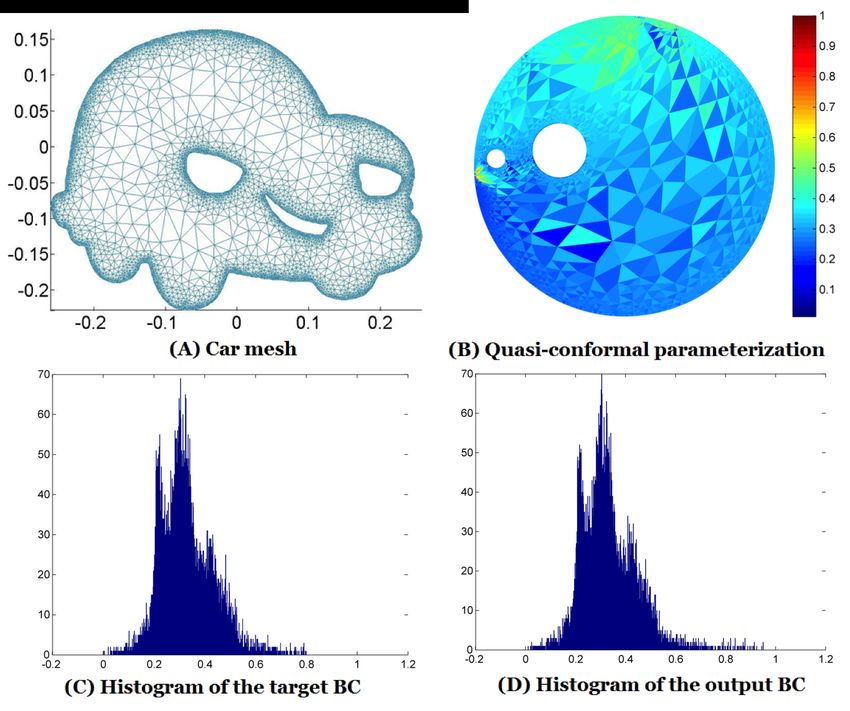
Quasi-conformal parameterization for Multiply-connected domains                                         3

has also been studied by Tutte [4]. The parameterization technique, which is now called the Tutte’s
embedding, was introduced. The bijectivity of the parameterization is mathematically guaranteed.
Floater [5] improved the quality of the parameterization by introducing specific weights, in terms of
area deformations and conformality.

    Besides, conformal parameterization has been extensively studied [6, 8–12, 27–29, 21]. Levy et al. [2]
proposed to compute the least square confomal parameterization through an optimiziation approach,
which is based on the least square approximation of the Cauchy-Riemann equations. Hurdal et al.
[12] proposed to compute the conformal parameterizations using circle packing and applied it to
register human brains. Porter [27] proposed to compute the conformal maps of simply-connected
planar domains by the interpolating polynomial method. Gu et al. [9–11] proposed to compute the
conformal parameterizations of Riemann surfaces for the purpose of registration using harmonic energy
minimization and holomorphic 1-forms. Later, the authors proposed the curvature flow method to
compute conformal parameterizations of high-genus surfaces onto their universal covering spaces, which
deforms the Riemmannian metric to the uniformization metric [23–25]. Wong et al. [39] also proposed
to apply the discrete Beltrami flow method to conformally parametrize high-genus surfaces to the
cannonical Poincare disk, through iteratively adjusting the generators in the uniformization domain.

    For multiply-connected open surfaces, various conformal parameterization techniques have been
recently developed. For example, the curvature flow method has been applied to compute the conformal
parameterization of a multiply-connected open domain onto a punctured disk [30, 32]. Hale et al.
[28] proposed to compute conformal maps to multiply-slit domains by using a Schwarz-Christoffel
formulation. DeLillo et al. [29] proposed a numerical method to compute the Schwarz-Christoffel
transformation for multiply-connected domains. Crowdy [42] proposed a formula for the generalized
Schwarz-Christofeel conformal mapping from a bounded multiply-connected circular domain to an
unbounded multiply-connected polygonal domain.

    Sometimes, when further constraints are enforced, exact conformal parameterizations may not be
achievable. In this case, quasi-conformal parameterizations have to be considered. Recently, various
algorithms for quasi-conformal parameterizations have been developed. For example, Mastin et al. [33]
proposed a finite difference scheme for constructing quasi-conformal mappings for arbitrary simply
and doubly-connected region of the plane onto a rectangle. In [34], Daripa proposed a numerical con-
struction of quasi-conformal mappings in the plane by solving the Beltrami’s equation. This method
was further extended to compute the quasi-conformal map of an arbitrary doubly connected domain
with smooth boundaries onto an annulus [35]. All of these methods deal with domains in the com-
plex plane. Recently, surface quasi-conformal maps have also been studied. Lui et al. [16] proposed to
compute quasi-conformal registration between hippocampal surfaces which matches geometric quan-
tities (such as curvatures) as much as possible. A method, called the Beltrami holomorphic flow, was
used to obtain the optimal Beltrami coefficient associated to the registration [15, 14, 19]. Wei et al.
[22] also proposed to compute quasi-conformal mapping for feature matching face registration. The
Beltrami coefficient associated to a landmark points matching parameterization was approximated.
However, either exact landmark matching or the bijectivity of the mapping cannot be guaranteed,
especially when very large deformations occur. In order to compute quasi-conformal mapping from the
Beltrami coefficients effectively, Quasi-Yamabe method was introduced, which applied the curvature
flow method to compute the quasi-conformal mapping [18]. The algorithm can deal with surfaces of
general topologies. Later, extremal quasi-conformal mappings, which minimize conformality distortion
has been proposed [26, 38] . For example, Lui et al. [26] proposed to compute the unique Teichmüller
extremal map between simply-connected or multiply-connected Riemann surfaces of finite type with
given Dirichlet boundary constraints. The proposed algorithm was applied for landmark-based surface
parameterization. Recently, Lipman et al. [36, 37] proposed to consider bounded distortion mappings,
which can be used to bijectively parameterize simply-connected or multiply-connected domains with
given Dirichlet boundary constraints. Most of the aforementioned existing algorithms parametrize
multiply-connected domains with Dirichlet boundary conditions given. In this work, our goal is to
propose a numerical method to quasi-conformally parameterize a multiply-connected domain onto
a simple/canonical parameter domain (such as the punctured disk) without enforcing any Dirichlet
boundary constraints.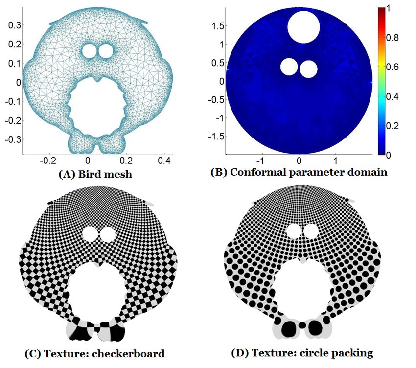
4                                                                               Kin Tat Ho, Lok Ming Lui

3 Objective

In this paper, our goal is to propose an effective numerical algorithm for quasi-conformal parame-
terizations of multiply-connected surfaces onto their corresponding canonical domains, which are the
punctured disks. The features of our proposed method are as follows.

Free of boundary constraints: Most of the existing parameterization models require setting Dirichlet
boundary constraints (that is, pointwise correspondences between the boundaries of the surface and the
parameter domain). In practice, it is challenging to prescribe a suitable Dirichlet boundary condition,
such that the overall conformality of the parameterization will not be affected. According to Theorem
1, given a Beltrami differential, a multiply-connected surface can be quasi-conformally parameterized
to a punctured disk. The geometry (radii and centers of the inner circles) of the punctured disk is
determined by the Beltrami differential. Motivated by this theorem, our algorithm computes the above
parameterization onto the canonical domain without setting any boundary constraints.

Type of the parameter domain: In many applications, parameterization of a surface onto a simple
parameter domain helps to simplify numerical computations on the original surface. Our algorithm
parameterize multiply-connected domains onto the canonical punctured disks. The punctured disk has
a simple geometry, which is a unit disk with several inner disks removed. By parameterizing a surface
onto the punctured disk, many numerical computations on the surface can be simplified.

Robustness and stablity: Our algorithm is robust, which can successfully work with meshes with poor
triangulations (such as meshes with skinny triangular faces). Also, our method is stable under different
initializations, even under a non-bijective initialization (see Figure 16).

Comparable computational time: The computational time of our algorithm is comparable to other
state-of-the-art algorithms, such as the curvature flow method.

Accuracy Experimental results shows that our algorithm can compute quasi-conformal parameteriza-
tion with good accuracy (see Section 7).

4 Mathematical background

In this section, we describe briefly some basic mathematical concepts closely related to this work. For
details, we refer the reader to [7].
    A surface S with a conformal structure is called a Riemann surface. Given two Riemann surfaces
M and N , a map f : M → N is conformal if it preserves the surface metric up to a multiplicative
factor called the conformal factor. An immediate consequence is that every conformal map preserves
angles. With the angle-preserving property, a conformal map effectively preserves the local geometry
of the surface structure. A generalization of conformal maps is the quasi-conformal maps, which
are orientation preserving homeomorphisms between Riemann surfaces with bounded conformality
distortion, in the sense that their first order approximations take small circles to small ellipses of
bounded eccentricity [7]. Mathematically, f : C → C is quasi-conformal provided that it satisfies the
Beltrami equation:
                                             ∂f        ∂f
                                                 = µ(z) .                                           (1)
                                             ∂z        ∂z
for some complex-valued function µ satisfying ||µ||∞ < 1. µ is called the Beltrami coefficient, which
is a measure of non-conformality. It measures how far the map at each point is deviated from a
conformal map. In particular, the map f is conformal around a small neighborhood of p when µ(p) = 0.
Infinitesimally, around a point p, f may be expressed with respect to its local parameter as follows:
                                   f (z) = f (p) + fz (p)z + fz (p)z
                                                                                                     (2)
                                        = f (p) + fz (p)(z + µ(p)z).

   Obviously, f is not conformal if and only if µ(p) 6= 0. Inside the local parameter domain, f may be
considered as a map composed of a translation to f (p) together with a stretch map S(z) = z + µ(p)z,
which is postcomposed by a multiplication of fz (p), which is conformal. All the conformal distortion of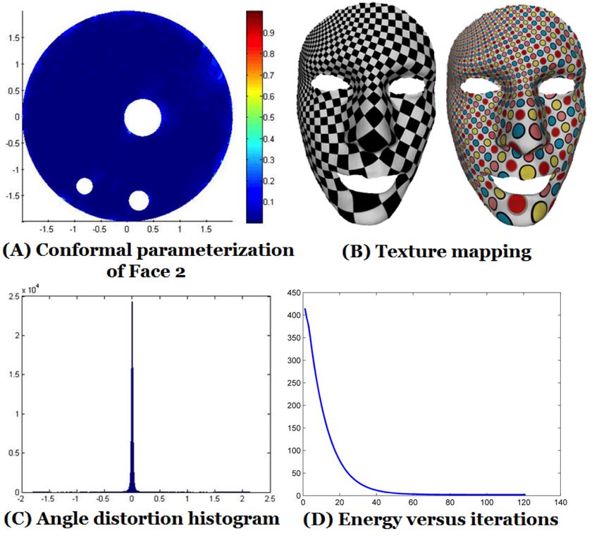
Quasi-conformal parameterization for Multiply-connected domains                                                     5

Fig. 1 The figure illustrates how the conformality distortion can be measured by the Beltrami coefficient. The picture
is adapted from [26].

Fig. 2 The figure illustrates how the surface quasi-conformal map is defined. The picture is adapted from [26].

S(z) is caused by µ(p). S(z) is the map that causes f to map a small circle to a small ellipse. From µ(p),
we can determine the angles of the directions of maximal magnification and shrinking and the amount
of them as well. Specifically, the angle of maximal magnification is arg(µ(p))/2 with magnifying factor
1 + |µ(p)|; The angle of maximal shrinking is the orthogonal angle (arg(µ(p)) − π)/2 with shrinking
factor 1 − |µ(p)|. Thus, the Beltrami coefficient µ gives us lots of information about the properties of
the map (See Figure 1).
    The maximal dilation of f is given by:
                                                         1 + ||µ||∞
                                               K(f ) =              .                                             (3)
                                                         1 − ||µ||∞
    Suppose f : Ω1 → Ω2 and g : Ω2 → Ω3 are quasi-conformal maps, whose Beltrami coefficients are
µf and µg respectively. Then, the Beltrami coefficient of the composition map g ◦ f : Ω1 → Ω3 is given
by:
                                               µf + rf (µg ◦ f )
                                      µg◦f =                                                       (4)
                                              1 + rf µf (µg ◦ f )
where rf = fz /fz .
    Given a Beltrami coefficient µ : C → C with kµk∞ < 1. There is always a quasi-conformal mapping
from C onto itself which satisfies the Beltrami equation in the distribution sense [7].
    Quasiconformal mapping between two Riemann surfaces S1 and S2 can also be defined. Instead of
the Beltrami coefficient, the Beltrami differential is used. A Beltrami differential µ(z) dz
                                                                                          dz on a Riemann
surface S is an assignment to each chart (Uα , φα ) of an L∞ complex-valued function µα , defined on
local parameter zα such that
                                                dzα             dzβ
                                       µα (zα )      = µβ (zβ )     ,                                  (5)
                                                dzα             dzβ
                                                                               dz
on the domain which is also covered by another chart (Uβ , φβ ). Here, dzαβ = dzdα φαβ and φαβ = φβ ◦φ−1
                                                                                                      α
(See Figure 2).
    Given a Beltrami differential µ(z) dz
                                       dz on a multiply-connected open surface S, the surface can always
be parameterized quasi-conformally onto a punctured disk with the prescribed Beltrami differential.
The geometry (centers and radii of the inner circles) depends solely on µ(z) dz  dz . More precisely,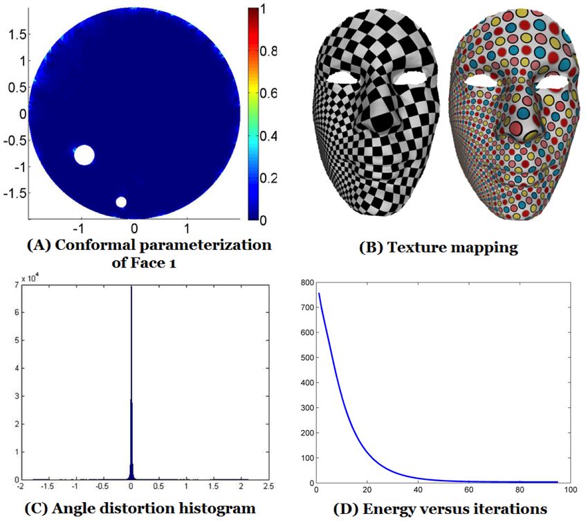
6                                                                                  Kin Tat Ho, Lok Ming Lui

Theorem 1 Suppose S is an open Riemann surface with multiple boundaries. Given a Beltrami differ-
ential µ(z) dz
            dz , there exist a quasi-conformal parameterization f : S → DS with the prescribed Beltrami
differential, where DS is a unit disk with circular holes (or the punctured disk). Two such parameter-
izations differ by a Möbius transform.

   In this work, our goal is to develop an effective numerical algorithm to compute such a quasi-
conformal parameterization.

5 Proposed method

The problem we address in this paper is to compute the quasi-conformal parameterization of a multiply-
connected domain S with a given Beltrami differential µ.
    Without loss of generality, we may assume S to be an open connected domain in R2 . Thus, we
can regard the Beltrami differential µ as the Beltrami coefficient. More specifically, if S is a multiply-
connected surface in R3 , we can easily map it onto an arbitrary 2D domain Ω using, for instance, the
IsoMap [13], the spectral conformal map algorithm [21] or the Beltrami holomorphic flow algorithm
with free boundary condition [15, 17]. Of course, the parameter domain Ω has an arbitrary shape (see
Figure 11). Denote the initial parameterization by φ : S → Ω, whose Beltrami differerential is µφ . Our
goal is to find a quasi-conformal parameterization f : Ω → DS between the 2D domain Ω and the
punctured disk DS , such that the composition map has Beltrami differential equals to µ. According
to equation (4), f should be a quasi-conformal map with Beltrami coefficient µf given by:

                                                1 µ − µφ
                                         µf =                 .                                        (6)
                                               rφ 1 − µµφ

   With this setting, we can now mathematically formulate our problem as follows: given a multiply-
connected domain S and a Beltrami coefficient µ : S → C, we look for a punctured disk :
                                                      n
                                                      [
                                           DS = D \         Bri (ci ).                                   (7)
                                                      i=1

where Bri (ci ) = {x ∈ D : |x − ci | < ri }, n
                                            S                       Tm
                                              i=1 Bri (ci ) ⊂ D and  i=1 Bri (ci ) = ∅ (0 < ri < 1 and
ci ∈ D ⊂ C), together with a quasi-conformal parameterization f : S → DS such that:

                                                ∂f     ∂f
                                                     =µ .                                                (8)
                                                ∂ z̄   ∂z
    Let r = (r1 , ..., rn ) ∈ Rn and c = (c1 , ..., cn ) ∈ Cn . (r, c) is called the conformal module of DS .
Solving the above problem (7) and (8) is challenging since both the conformal module of the target
parameter domain and the quasi-conformal map f are unknown.
    In this work, we propose a variational approach to solve the problem. Let ∂S = {γ0 , γ1 , ..., γn }
where γ0 is the outermost boundary, γ1 , ..., γn are the inner boundaries. Equation (8) is equivalent to
solving:
                                                               ∂f       ∂f
                                   f = argminf :S→DS {||            − µ ||∞ }.
                                                               ∂ z̄     ∂z
    Hence, we can set up our problem as minimizing:
                                                      Z
                                                          ∂f         ∂f
                                    EB (f, r, c) = { |          − µ |p dS},                               (9)
                                                        S ∂ z̄       ∂z

subject to the constraints that:
(1) f |γi (γi ) = ∂Bri (ci ) for i = 1, 2, ..., n ,
(2) f |γ0 (γ0 ) = ∂D and
(3) ||µ(f )||∞ := || ∂f     ∂f
                     ∂ z̄ / ∂z ||∞ < 1.
    The optimal map is called the quasi-conformal parameterization (QCMC) for the multiply-connected
domain. Note that if we set p to be large enough, the optimization problem gives a good approxima-
tion of the quasi-conformal parameterization solving equation (8). In practice, we set p = 2 and it is
found that the obtained optimal map is already a close approximation of the desired quasi-conformal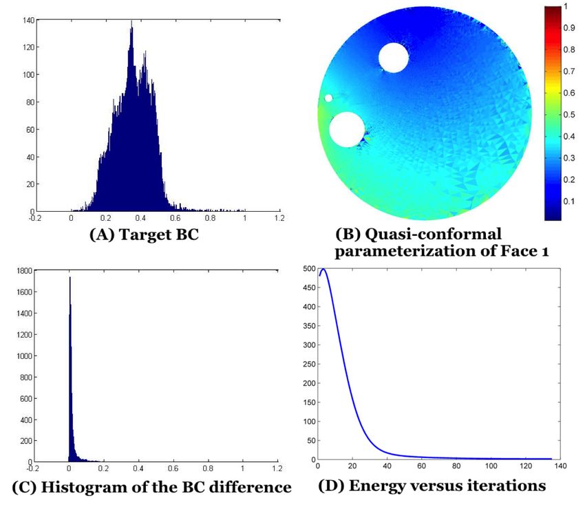
Quasi-conformal parameterization for Multiply-connected domains                                            7

parameterization. In this case, the optimal map is a least square quasi-conformal parameterization
(LSQCMC) for S.
   Furthermore, constraint (3) guarantees the map f is folding-free (locally bijective). This can be
explained as follows. In fact, the Jacobian Jf of f is closely related to the Beltrami coefficient:
                                             2            2            2
                                        ∂f           ∂f           ∂f
                                 Jf =            −            =            (1 − |µf |2 ).               (10)
                                        ∂z           ∂z           ∂z
    Since ||µ(f )||∞ < 1 , we have |Jf | > 0 everywhere. Hence, by the inverse function theorem, f is
locally bijective. In fact, |Jf | > 0 also implies f induces a Riemannian metric on S. More precisely,
with a Beltrami differential µ with ||µ||∞ < 1, an auxiliary metric can be defined on S by |dz + µdz|2 ,
where |dz|2 is the original local metric on S. Under the auxiliary metric, f is a conformal map [18].
The fundamental theory of conformal mapping states that every multiply-connected Riemann surface
with a valid Riemannian metric can be mapped by a conformal and one-to-one transformation onto a
punctured disk. Hence, f that solves the original problem satisfying equations (7) and (8), is in fact a
global bijection.
   The optimization problem (9) is not a standard Lp -minimization problem. It involves both the
optimizations of the quasi-conformal map f together with the boundary constraints. In other words,
we simultaneously look for the best conformal module for the boundary constraints and the optimal
quasi-conformal map f satisfying the constraints such that the energy EB is minimized. Theoretically,
there exists a conformal module and quasi-conformal map f such that EB = 0.
   In this paper, we propose to solve this optimization problem (9) by an iterative descent algorithm,
which considers both the map f and the conformal module (r, c) as variables simultaneously, to
minimize EB . We will explain the proposed iterative method in details in the following subsections.

5.1 Energy minimization with fixed conformal module

In this subsection, we first discuss how we can iteratively adjust the map f to minimize EB with fixed
conformal module, which is a slightly      simpler problem than our original problem. More specifically,
given a punctured disk DS = D \ n
                                   S
                                     i=1 Bri (ci ), we look for an optimal map f : S → DS that minimizes
EB . To solve this problem, we propose to iteratively find a sequence of maps from an initial map,
which converges to our desired quasi-conformal parameterization minimizing EB . Let f ν be an initial
map (not necessarily bijective) with Beltrami coefficient ν. Our goal is to deform f ν to another map
f such that it reduces EB (f ). Let δf = f − f ν and let A(µ) be the differential operator defined by
          ∂      ∂
A(µ) := ∂z  − µ ∂z . Then, the energy functional EB (f ) can be reformulated as follows:
                                                     Z
                                         0
                             EB (f ) = EB   (δf ) :=    |A(µ)δf + A(µ)f ν |p dS.                    (11)
                                                          S

     Using the above formualtion, we propose to iteratively deform an initial map g 0 : S → DS to an
optimal quasi-conformal map g ∗ : S → DS , whose Beltrami coefficient is closest to the given µ in the
Lp -sense. The initial map can be chosen as the harmonic map with boundary pointwise correspondence
given by the arc-length parameterization. Let the Beltrami coefficient of g 0 be ν0 . Our goal is to deform
g 0 to g 1 = g 0 + δg 0 , whose Beltrami coefficient is closer to the target µ in the Lp -sense. According to
new formulation (11), it can be achieved by finding a δg 0 that minimizes
                                                  Z
                                      0
                                    EB  (δg 0 ) =   |A(µ)δg 0 + A(µ)g 0 |p dS                            (12)
                                                     S

subject to the boundary constraints: g |γi (γi ) = ∂Bri (ci ) and g 1 |γ0 (γ0 ) = ∂D.
                                         1

    The boundary constraints can be enforced as follows. In general, points on the boundary γi of S
are allowed to move along the target boundary γi0 ⊂ ∂DS (γi0 = ∂Bri (ci ) if i = 1, 2, ..., n and γ00 = ∂D).
In other words, we need to restrict the movement to be the tangential direction of the target boundary
component. Let uk ∈ γi be a point on the boundary component γi of S. We require that the variation
δg 0 on uk satisfies the following:
                                       δg 0 (uk ) = tk Tγk0 (g 0 (uk )),                                (13)
where Tγk0 (g 0 (uk )) is the unit tangent vector of γk0 at g 0 (uk ) and tk ∈ R is a variable measuring the
length of δg 0 at uk (how far it deforms the map g 0 ).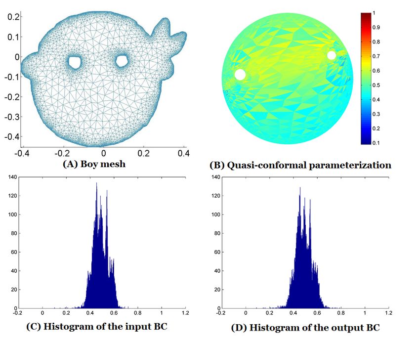
8                                                                                      Kin Tat Ho, Lok Ming Lui

   Note that the target boundary component γk0 is a circle. Suppose γk0 is a circle centered at ck with
radius rk , the equation can be simplified as:

                                                            g 0 (uk ) − ck
                                         δg 0 (uk ) = itk                  .                                (14)
                                                                  rk

   With this setting, our problem becomes solving the optimization problem (12) subject to the
boundary constraint (14). In practice, we choose p = 2. In this case, the problem becomes a least
square minimization problem. In the discrete case, it is equivalent to a sparse linear system.
   Now, as the boundary point uk moves along the tangential direction, it may leave the target
boundary γk0 by a short distance. Thus, we project it back to γk0 by solving:
                                                                                   2
                              g 1 (uk ) = argminx∈γk0 g 0 (uk ) + δg 0 (uk ) − x                            (15)
                                                                                   2

Since γi0 is simply a circle, this process is just rescaling the distance between g 0 (uk ) + δg 0 (uk ) and ck
to rk as follows:
                                            g 0 (uk ) + δg 0 (uk ) − ck
                                g 1 (uk ) = 0                           · rk + c k .                       (16)
                                           kg (uk ) + δg 0 (uk ) − ck k
    Note that, according to our setting, we only allow the boundary points to move a bit along the
                                                                  0
target boundary. Although g 1 := g 0 + δg 0 reduces the energy EB   , it is unlikely the optimal map that
solves the optimization problem (12) and (14).
    Therefore, we repeat the procedure. More precisely, suppose g k is obtained at the k-th iteration.
                                                               0
We can obtain a new map g k+1 := g k + δg k that reduces EB       by minimizing ||A(µ)δg k + A(µ)g k ||pp
subject to the boundary constraint (14). As a result, we obtain a sequence of maps {g k }∞       k=1 with
Beltrami coefficients {µk }∞
                           k=1 , which converges to the desired  optimal   map.
    In summary, the iterative scheme for computing the optimal quasi-conformal map with fixed con-
formal module of the target parameter domain can be described as Algorithm 1.

    Algorithm 1: Energy minimization for fixed conformal module
      Data: triangular mesh of the source domain S, target domain DS and target Beltrami
              coefficient µ.
      Result: g ∗ : S1 → DS .
                  0
    1 Initialize g to be a harmonic map.
                                          0    0
    2 Calculate the Beltrami coefficient µ of g .
    3 while kµn − µn−1 k >  do
    4     Find δg n−1 that optimizes (12) subject to the constraint (16).
    5     Set g n = g n−1 + δg n−1 .

5.2 Adjustment of the conformal module

One of the main challenges for solving the optimization problem (9) is that the conformal module of
the target domain is not fixed. In other words, the geometry of the target parameter domain can be
                                        0
adjusted to further minimize EB           .
     To solve this problem, our strategy is to regard the conformal module as another variable, and let
it vary together with the map during the optimization process. In other words, we need to incorporate
the conformal module into the energy functional of the optimization problem.
     Given a multiply-connected domain S, we first obtain an intial guess of the conformal module
(r0 , c0 ). r0 = (r0 , r1 , ..., rn )T and c0 = (c0 , c1 , ..., cn )T can be chosen as follows. For each γi (i =
0, 1, 2, ..., n), we find a circle approximating γi . In this way, we obtain a circle domain (a disk with n
inner disks removed). The circle domain is then normalized such that the outermost boundary becomes
the unit circle. The initial guess r0 and c0 are then         S obtained,0 and the initial guess of the parameter
domain DS     0
                 is obtained. In other words, DS 0
                                                    =D\ n        i=1 Bri0 (ci ).
Quasi-conformal parameterization for Multiply-connected domains                                            9

                                                                                       i
    Our problem can now be regarded as finding a sequence of punctured disks DS          and maps g i , which
iteratively minimizes EB (g, r, c). To do this, we propose to give an extra freedom to the variation δg i
on the boundary component γk (k = 1, 2, ..., n). The main idea is to allow ri and ci to vary. More
specifically, the translation of the center from cik to cik +∆cik can be considered as all points on γk being
translated by ∆cik . Also, the scaling of the radius from rki to rki + ∆rki can be regarded as all points on
γk being moved along the radial direction by ∆rki . Therefore, the variation δg i on the boundary point
uk ∈ γk can be formulated as:

                                                                                 uk − cik
                            δg i (uk ) = tk Tγk0 (g i (uk )) + ∆cik +                     ∆rki .        (17)
                                                                                 uk − cik

    Note that the target boundary of the outermost boundary is always fixed to be the unit circle.
Thus, the above formulation does not apply to γ0 .
    We then minimize the energy functional (12) subject to the boundary constraint (14) and (17).
This new optimization problem involves new variables ∆ci and ∆ri , which are the perturbation of the
                                                               i
centers and radii (conformal module) of the inner disks of DS    . With this setting, we simultaneously
                    i                              i i                 0
optimize the map g and the conformal module (r , c ) to optimize EB      .
                              i
    Note that the variation δg for the interior points is a complex number, which can be represented
by two real scalars (one for the real part and one for the imaginary part). Besides, the variation δg i
for the boundary points must be a scalar multiple of the tangential direction of the boundary and can
                                                                         fi . We can write δg
be represented by one real scalar. Denote the representation of δg i by δg                  fi as:

                                 fi = [xi1 , y1i , xi2 , y2i , ..., xim , ym
                                 δg                                        i
                                                                             , ti1 , ..., tip ],        (18)

                        √
where δg i (vj ) = xij + −1yji for an interior vertex vj and tis is the representation of δg i (vs ) (using
equation (17)) for a boundary vertex vs .
    A linear operator K i transforms the representation δg   fi back to δg i . K i depends on the variables
   i          i
∆r and ∆c . Hence, our problem can be formulated as minimizing the following energy functional
     fi :
over δg
                                                           Z                         p
                   E    fi , ∆ri , ∆ci ) := EB
                    eB (δg                   0      fi ) =
                                               (K i δg                fi + A(µ)g i dS.
                                                              A(µ)K i δg                               (19)
                                                                       S

                                            fi reduces storage requirement. More importantly, the
    Representing δg i by its representation δg
above formulation allows us to incorporate the conformal module into the energy functional of the
optimization problem. In practice, we solve (19) by taking p = 2. In other words, we solve (19) by the
least square method.
    The overall iteratve scheme is summarized in Algorithm 2.

 Algorithm 2: Overall algorithm of QCMC
   Data: triangular mesh of source domain S, target Beltrami coefficient µ, tolerance .
   Result: Quasi-conformal parameterization g ∗ : S → DS .
 1 Initialize D0 to be punctured disk with the same topology of S.
               0
 2 Initialize g : Ω → D0 to be the harmonic map.
 3 while kµn+1 − µn k >  do
 4     Calculate tangent vector and outward normal vector at boundary.
 5     Construct constraint matrix K n .
 6     Find δg n , ∆cn and ∆rn by solving (19) with Lp -minimization.
 7                               fn (e.g. take t = 0.5).
       Let g n+1 = g n + t · K n δg
                                g n (uk )−cn
 8     Update g n+1 (uk ) ←                k
                                                · rkn + cn
                                                         k for all uk ∈ γk .
                              kgn (uk )−cnk k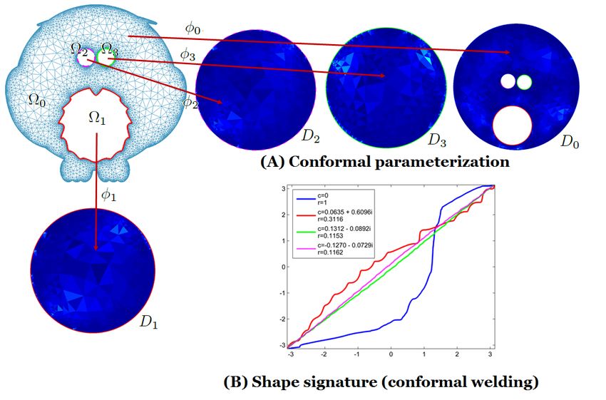
10 Kin Tat Ho, Lok Ming Lui
6 Numerical implementation
In this section, we will describe briefly how the proposed algorithm introduced in Section 5 can be
implemented. The major components of the proposed algorithms are the constructions of A and K n in
the discrete setting. In the following subsection, we will describe how to discretize the two operators.
In practice, 2D domains or surfaces in R3 are usually represented discretely by triangular meshes.
Suppose M is the surface mesh representing the surface S. We define the set of vertices on M by
V = {vi }n m
i=1 . Similarly, we define the set of triangular faces on M by F = {Tj }j=1 . Our goal is to look
for a quasi-conformal parameterization f : M → C. We further introduce the following notions.
– U is a 2n × 1 vector. It stores the position of {f (vi )}n i=1 , namely,
U = (Re(f (v1 )), Re(f (v2 )), ..., Re(f (vn )), Im(f (v1 )), Im(f (v2 )), ..., Im(f (vn )))T .
– Vn is a 2n × 1 vector. It stores the vector field acting on U at the nth iteration.
∂ ∂
– A is a 2m×2m matrix, which is the matrix representation of the differential operator: A = ∂z −µ ∂z .
6.1 Construction of the matrix representation A of A
In practice, we consider the parameterization f : M → D to be piecewise linear, where D is the
triangulation mesh of a punctured disk. In other words, we regard the restriction of f on each trianguar
face Ti as an affine transform. Hence,
∂fi ∂fi
fi := f |Ti = z+ z + δi .
∂z ∂z
∂fi ∂fi
Let the vertices of Ti be {w1 , w2 , w3 } and vertices of fi (Ti ) be {z1 , z2 , z3 }. Then, ∂z and ∂z satisfy
the following linear system :
∂fi
w1 w1 1 ∂z z1
w2 w2 1 ∂fi = z2 .
∂z
w3 w3 1 δi z3
The above linear system can be reduce to:
∂fi
w2 − w1 w2 − w1 ∂z z2 − z1
∂fi = ,
w3 − w1 w3 − w1 ∂z
z3 − z1
Hence,
∂fi −1
∂z w2 − w1 w2 − w1 z2 − z1
∂fi = .
∂z
w3 − w1 w3 − w1 z3 − z1
By solving this linear system, we get ∂f ∂fi
∂z and ∂z . With that, Afi can be constructed by Afi =
i
∂fi ∂fi
∂z − µ(Ti ) ∂z .
Also, (Re(Af1 ), Re(Af2 ), ..., Re(Afm ), Im(Af1 ), Im(Af2 ), ..., Im(Afm ))T can be written as AU ,
where A ∈ M2m×2m (R). Hence, the matrix representation A of A can be obtained.
6.2 Construction of the boundary constraint matrix K
Now, we discuss how to construct the boundary constraint matrix K.
Let Iint = {i1 , i2 , ..., ir } be the indices of all interior vertices.
Let Ibdy = {ib1 , ..., ibs } be the indices of all boundary vertices.
Denote the tangent vector of the boundary vertex vibk by tk ∈ C.
Note that r+s = n. Under the boundary constraints, the admissible variation δg can be represented
f ∈ Rn+r . In particular, the variation on the interior vertices depends on two scalar
by a vector δg
variabes (real and imaginary parts of the vector field). Hence, 2r scalars are required to represent the
variation on the interior vertices. For the boundary vertices, the variation must be a scalar multiple of
the tangential direction and it depends on one scalar variable. Thus, s scalars are required to representQuasi-conformal parameterization for Multiply-connected domains 11
the variation on the boundary vertices. All together, 2r + s = n + r scalars are required to represent
the admissible variation.
The boundary constraint matrix K transforms the variation representation δg f into the admissible
variation δg. The matrix K can be regarded as a 2n × (n + r) sparse matrix, which can be constructed
as follow :
For j = 1, 2, ..., r ,
Ki,j =1
(20)
Kn+i,j = 1
For j = 1, 2, ..., s ,
Kibj ,r+j = Re(tj )
(21)
Kn+ibj ,r+j = Im(tj )
f ∈ R2n becomes a vector of size 2n. The first n entries represent the real
In this way, δg := K δg
part of the variation and the last n entries represent the imaginary part of the variation.
7 Experimental results
In this section, we test our proposed algorithm to compute conformal and quasi-conformal parame-
terizations of synthetic data and real human face surfaces. All our experiments are carried out on a
desktop with following specification:
Hardware Specification
Processor AMD A8-6600K (3.9GHz ×4)
Memory 8GB DDR3-1600
Operating system Window 8 Home Pre. 64bit
Experiment perform Matlab 2013a
GPU assisted computation No
7.1 Synthetic 2D domains
We first examine our algorithm on multiply-connected 2D domains.
Example 1 In this example, we compute the least square conformal parameterization of a 2D triply-
connected frog mesh (Figure 3(A)) and a 2D bird mesh (Figure 5(A)). The conformal parameterizations
are shown in (B). The colormaps are given by the norms of the Beltrami coefficients. The blue color
indicates that the Beltrami coefficient is close to 0, meaning that the parameterization is indeed
conformal. Using the conformal parameterization, we map the checkerboard texture and circle packing
texture onto the frog mesh, as shown in (C) and (D).
Note that the right angle of the checkerboard pattern are well-preserved, meaning that the pa-
rameterizations are angle-preserving. The circle pattern of the circle packing texture is also preserved.
It means that under the conformal parameterization, infinitesimal circles are mapped to infinitesimal
circles as expected.
Figure 4(A) and Figure 6(A) show the histograms of the angle distortion under the parameteriza-
tions. They accumulte at 0, meaning that the parameterization is indeed angle-preserving. The energy
versus iterations using our proposed algorithm is shown in (B). EB decreases as iteration increases.12 Kin Tat Ho, Lok Ming Lui
Fig. 3 (A) shows the frog mesh. (B) shows the conformal parameterization. (C) shows the texture mapping of the
checkerboard using the obtained conformal parameterization. (D) shows the texture mapping of the circle packing
pattern.
Fig. 4 (A) shows the histogram of the angle distortion under the conformal parameterization of the frog mesh. (B)
shows the energy versus iterations.
Example 2 We test our algorithm to compute the least square quasi-conformal parameterizations of a
2D triply-connected boy mesh (Figure 7(A)) and a 2D car mesh with three inner holes (Figure 9(A)).
The quasi-conformal parameterizations are shown in (B). (C) shows the histogram of the norms of
the target Beltrami coefficients and (D) shows the histograms of the norms of the output Beltrami
coefficients.
We can see that the Beltrami coefficients of the quasi-conformal parameterizations are closely
resemble to our target Beltrami coefficients. Also, Figure 8 and Figure 10 show that the histograms
of the errors between the target and output Beltrami coefficients accumulate at 0, indicating that the
obtained maps are good approximations to our desired quasi-conformal parameterizations. The energy
versus iterations using our proposed algorithm is shown in (B).
7.2 Multiply-connected Riemann surfaces
We next examine the algorithm on multiply-connected Riemann surfaces.
Example 3 In this example, we test the algorithm to compute the conformal parameterizations of two
multiply-connected human faces onto punctured disks . The human faces are shown in Figure 11, andQuasi-conformal parameterization for Multiply-connected domains 13
Fig. 5 (A) shows the bird mesh. (B) shows the conformal parameterization. (C) shows the texture mapping of the
checkerboard using the obtained conformal parameterization. (D) shows the texture mapping of the circle packing
pattern.
Fig. 6 (A) shows the histogram of the angle distortion under the conformal parameterization of the bird mesh. (B)
shows the energy versus iterations.
the surfaces are conformally embedded into R2 with free boundary condition. The embedded domains
are then conformally parameterized onto the puntured disk.
The conformal parameterizations of the human faces are shown in Figure 12(A) and Figure 13(A).
The texture maps (checkerboard and circle packing) using the conformal parameterizations are shown
in (B). The right angle structure is well-preserved and the parameterizations map infinitesimal circles
to circles. (C) shows the histogram of angle distortion, which shows that the parameterization is
angle-preserving. (D) shows the energy versus iterations.
Example 4 Now, we compute the quasi-conformal parameterizations of these two faces. The norms of
the target Beltrami differentials are shown in Figure 14(A) and Figure 15(A). The quasi-conformal
parameterizations are shown in (B). The colormaps show the norms of the Beltrami differentials of
the parameterizations. (C) shows the histograms of the errors between the target and output Beltrami
differentials. They accumulate at 0, meaning that the computed quasi-conformal parameterizations
are accurate. (D) shows the energy versus iterations.14 Kin Tat Ho, Lok Ming Lui
Fig. 7 (A) shows the boy mesh. (B) shows the quasi-conformal parameterization. (C) shows the histogram of the
target Beltrami coefficient. (D) shows the histogram of the norm of the output Beltrami coefficient.
Fig. 8 (A) the histogram of the error between the target and output Beltrami coefficients for the boy mesh example.
(B) shows the energy versus iterations.
Mesh Faces Vertice Time spent Mean(|µ|) Std(|µ|) # of flips
Frog 10603 5918 6.05 s 0.0124 0.0148 0
Boy 15164 8699 5.90 s 0.0196 0.0214 0
Cat 7857 4411 5.06 s 0.0247 0.0297 0
Bird 10965 6210 7.57 s 0.0258 0.0378 0
Car 10267 5805 8.57 s 0.0264 0.0282 0
Table 1 Computational details of the proposed algorithm
7.3 Computational time, stability and comparisons
Table 1 reports the computational details of our proposed algorithm. For meshes with about 10k faces,
our proposed algorithm can generally obtain the parameterization onto the punctured disk with in
10 seconds. All the parameterization results have no overlapping faces, which means the obtained
parameterizations are indeed bijective.
We also study the stability of our proposed algorithm under different initializations. It is observed
that our algorithm converges to the same solution with different initializations, even for a non-bijective
initial map. Figure 16(A), (B) and (C) shows three different initializations for the conformal param-
eterization of the frog mesh (as in Figure 3(A)). Note that the initializations are all different, whose
parameter domains have different conformal modules. Besides, two initial maps, namely (B) and (C),
are non-bijective. With these three different initializations, our algorithm converges to the same pa-Quasi-conformal parameterization for Multiply-connected domains 15 Fig. 9 (A) shows the car mesh. (B) shows the quasi-conformal parameterization. (C) shows the histogram of the target Beltrami coefficient. (D) shows the histogram of the norm of the output Beltrami coefficient. Fig. 10 (A) shows the histogram of the error between the target and output Beltrami coefficients for the car mesh example.(B) shows the energy versus iterations. Fig. 11 (A) shows a triply-connected human face and its conformal embedding with free boundary condition in R2 . (B) shows the human face with three interior regions removed and its conformal embedding with free boundary condition in R2 . rameterization (up to a rotation), which are shown in (D), (E) and (F) respectively. Also, the optimal parameterization becomes bijective, even though the initial map is non-bijective. Finally, we compare our proposed algorithm with the Ricci flow (RF) method [23] and the inverse curvature Ricci flow (IDRF) method [24]. The results are reported in Table 2. As shown in the table, our method is stable under different regularities of the triangulations. On the contrary, both RF and IDRF fail on some meshes without remeshing. After improving the regularity of the triangulation through a remeshing process, RF and IDRF can be used to parameterize some of the meshes onto the punctured disks. To compare the quality of the conformal parameterization, we compute the mean
16                                                                                   Kin Tat Ho, Lok Ming Lui

Fig. 12 (A) shows the conformal parameterization of human face 1. The texture map (checkerboard and circle
packing) using the conformal parameterization is shown in (B). (C) shows the histogram of angle distortion. (D)
shows the energy versus iterations.

Fig. 13 (A) shows the conformal parameterization of human face 2. The texture map (checkerboard and circle
packing) using the conformal parameterization is shown in (B). (C) shows the histogram of angle distortion. (D)
shows the energy versus iterations.

and standard derivation of the angle distortion. From the table, it can be observed that our proposed
algorithm outperforms RF and IDRF.

8 Applications

In this section, we show some applications of the conformal and quasi-conformal parameterizations.
Quasi-conformal parameterization for Multiply-connected domains                                                   17

Fig. 14 Quasi-conformal parameterization of the human face 1. (A) shows the norm of the target Beltrami differential.
The quasi-conformal parameterization is shown in (B). The colormap shows the norm of the Beltrami differential of
the parameterization. (C) shows the histogram of the error between the target and output Beltrami differentials. (D)
shows the energy versus iterations.

Fig. 15 Quasi-conformal parameterization of the human face 2. (A) shows the norm of the target Beltrami differential.
The quasi-conformal parameterization is shown in (B). The colormap shows the norm of the Beltrami differential of
the parameterization. (C) shows the histogram of the error between the target and output Beltrami differentials. (D)
shows the energy versus iterations.

8.1 Surface remeshing

Surface remeshing refers to the process of improving the quality of the triangulation. This procedure
is necessary in numerical computations to improve the accuracies of numerical solutions. A common
technique to perform remeshing is done by parameterizing the surface onto a simple parameter domain
(usually in R2 ). A regular mesh can be built on the simple parameter domain and the remeshing can be
18 Kin Tat Ho, Lok Ming Lui
Fig. 16 Conformal parameterizations of the frog mesh using our proposed method under different initializations.
(A), (B) and (C) show three different initializations. (D), (E) and (F) show the obtained conformal parameterizations
with initializations (A), (B) and (C) respectively.
Mesh Ordinary RF [23] IDRF [24] QCMC
mean(µ)/std(µ) mean(µ)/std(µ) mean(µ)/std(µ)
Frog 0.1907/0.1548 0.0164/0.0196 0.0129/0.0164
Boy 0.1647/0.1263 0.0212/0.0288 0.0203/0.0241
Cat 0.1852/0.1545 0.0252/0.0284 0.0233/0.0255
Bird fail fail 0.0245/0.0401
Car 0.1881/0.1488 0.0277/0.0311 0.0253/0.0270
2hole face 0.2937/0.2625 fail 0.0114/0.0351
2hole face (remeshed) 0.2402/0.2412 0.0097/0.0175 0.0051/0.0058
3hole face 0.3079/0.2591 fail 0.0195/0.0516
3hole face (remeshed) 0.2281/0.2205 0.0137/0.0220 0.0057/0.0070
Table 2 Comparison of different algorithms.
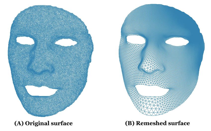
done through interpolation. Figure 17(A) shows the original surface mesh. We conformally parameterize
the surface onto a punctured disk and a regular mesh is built on the parameter domin. Remeshing
is then done by interpolation. The remeshed surface is shown in (B). Figure 18(left) shows the zoom
in of the triangulation mesh of the original surface. The right shows the zoom in of the triangulation
mesh of the remeshed surface. The quality of the triangulation is much improved.
8.2 Surface registration
Quasi-conformal surface maps have been used for surface registration. Computing quasi-conformal
surface maps between multiply-connected surfaces is challenging, due to the complicated topologies
of the surfaces. By parameterizing the surfaces onto the punctured disk, the computation can be
simplified. Figure 19(A) and (B) show two metal sheets, which are doubly-connected. Given a Beltrami
differential on the metal sheet 1, our goal is to compute the quasi-conformal surface map between the
metal sheets. To do this, we first quasi-conformally parameterize the metal sheet 1 with the prescribed
Beltrami differential onto the annulus. The parameterization is as shown in (C) and the colormap is
given by the norm of the Beltrami differential. Then, we parameterize the metal sheet 2 conformallyQuasi-conformal parameterization for Multiply-connected domains 19 Fig. 17 (A) shows the original surface mesh. (B) shows the remeshed surface. Fig. 18 The left shows the zoom in of the triangulation mesh of the original surface in Figure 17(A). The right shows the zoom in of the triangulation mesh of the remeshed surface. Fig. 19 (A) shows the metal sheet 1. (B) shows the metal sheet 2. (C) shows the quasi-conformal parameterization of the metal sheet 1. (D) shows the conformal parameterization of the metal sheet 2. The surface quasi-conformal map between the metal sheets can be obtained by the composition map. onto an annulus, as shown in (D). In this way, the parameter domains of metal sheet 1 and metal sheet 2 are conformally equivalent. Hence, their conformal modules are the same up to a Möbius transformation. As shown in the figure, the inner radii of the two annulus are both approximately 0.6401. By the composition of the parameterizations, the quasi-conformal surface map between the two metal sheets can be obtained. Figure 20 shows the visualization of the surface quasi-conformal map between the metal sheets using texture mapping. The circle packing pattern on the original metal sheet is mapped onto the target metal sheet. Infinitesimal circles are mapped to infinitesimal ellipses.
20                                                                                         Kin Tat Ho, Lok Ming Lui

Fig. 20 Visualization of the surface quasi-conformal map between the metal sheets. The circle packing pattern on the
original metal sheet is mapped onto the target metal sheet. Infinitesimal circles are mapped to infinitesimal ellipses.

    Furthermore, by parameterizing the multiply-connected surfaces onto the punctured disk, surface
registration can be computed easily on the simple parameter domains. Figure 21(A) and (B) show two
different human faces S1 and S2 . We look for a geometric matching surface registration between them
that matches curvatures. More specifically, we look for a diffeomorphism f : S1 → S2 that minimizes:
                                         Z                 Z
                       Egeometric (f ) =     |µ(f )|4 dS +   (H1 − H2 (f ))2 dS                  (22)
                                                 S1                 S1

where H1 and H2 are the mean curvatures on S1 and S2 respectively. The first term minimizes the
conformality (local geometric) distortion of the map f . The second term minimizes the curvature
mismatching under the registration.
    We first conformally parameterize the two surfaces onto their canonical parameter domains, which
are shown in (D) and (E). The colormaps on the two parameter domains are given by the mean
curvatures of the two human faces. We then perform intensity-matching registration to find a mapping
between the parameter domains that matches the curvature intensities. Using the obtained mapping,
we transform source parameter domain to the target conformal parameter domain. The transformed
domain is shown in (F). Finally, the surface registration can be obtained from the composition map.
In (C), we map the curvature on the source surface to the target surface using the obtained surface
registration. Note that the corresponding regions (high curvature regions) are consistently matched. It
indicates that the obtained registration is geometric matching. Figure 22 shows the energy plots versus
iterations during the process of registration between the parameter domains. (A) shows the curvature
mismatching energy Ecurvature versus iterations. It decreases as iteration increases until the optimal
state is reached. (B) shows the total energy Egeometric versus iterations.

8.3 Shape signatures of multiply-connected objects

Conformal parameterization of the 2D multiply-connected domain can be used to compute the shape
signature representing the 2D shape. With the conformal parameterizations, conformal weldings can
be computed, which can be used to define the shape signature [20]. Figure 23(A) shows the frog mesh.
It consists of three sub-domains, namely, Ω0 , Ω1 and Ω2 , together with the infinite domain Ωoutside
outside the outermost boundary. Their conformal parameterizations, φ0 : Ω0 → D0 , φ1 : Ω1 → D1 ,
φ2 : Ω2 → D2 and φoutside : Ωoutside → D, are computed. The conformal weldings can be obtained
from the conformal parameterizations. More precisely, the conformal weldings can be computed as
follows: f01 := φ1 ◦ φ−1   1     1              −1   1      1                           −1   1
                      0 : S → S , f02 := φ2 ◦ φ0 : S → S and foutside := φoutside ◦ φ0 : S → S .
                                                                                                   1

The conformal wedings together with the conformal module of D0 form the shape signature of the frog
mesh, as shown in (B).
    Figure 24(A) shows the bird mesh and the conformal parameterizations of different sub-domains
of the bird mesh. Using the conformal parameterizations, conformal weldings can be defined. The
conformal weldings together with the conformal module of D0 define the shape signature of the frog
mesh, which are shown in (B).

9 Conclusion

We address the problem of finding the quasi-conformal parameterization (QCMC) for a multiply-
connected 2D domain or surface embedded in R3 . Our goal is to map the multiply-connected domain
one-to-one and onto a simple parameter domain. According to the quasi-conformal Teichmüller theory,
Quasi-conformal parameterization for Multiply-connected domains 21 Fig. 21 (A) and (B) show the human face 1 and human face 2, whose colormaps are given by their mean curvature. (C) shows the surface registration between the human faces. (D) shows the conformal parameterization of face 1. (E) shows the conformal parameterization of face 2. (E) shows the registration between the conformal parameter domians. Fig. 22 Energy plots for the surface registration example. (A) shows the curvature mismatching versus iterations. It decreases as iteration increases until the optimal state is reached. (B) shows the total energy Egeometric versus iterations. given a prescribed Beltrami differential measuring the conformality distortion, a multiply-connected domain can be quasi-conformally parameterized onto a punctured disk. The center and radii of the inner circles, which is called the confomal module, can be uniquely determined up to a Möbius trans- formation. In this paper, we propose an iterative algorithm to simultaeneously look for the conformal module and the optimal quasi-conformal map. The key idea is to minimize the Beltrami energy with the conformal module incorporated. By incorporating the conformal module into the energy functional of the optimization problem, the quasi-conformal map and the conformal module can be simultaneously optimized. The optimal solution is our desired quasi-conformal parameterization onto a punctured disk. The parameterization of the multiply-connected domain simplifies numerical computations and has important applications in various fields, such as in computer graphics and visions. Experiments have been carried out on synthetic data together with real multiply-connected Riemann surfaces. Re- sults show that our proposed method can efficiently compute quasi-conformal parameterizations of multiply-connected domains and outperforms other state-of-the-art algorithms. Applications of the parameterization technique have also been shown.
You can also read