Enhancing Target Speech Based on Nonlinear Soft Masking Using a Single Acoustic Vector Sensor - MDPI
←
→
Page content transcription
If your browser does not render page correctly, please read the page content below
applied
           sciences
Article
Enhancing Target Speech Based on Nonlinear Soft
Masking Using a Single Acoustic Vector Sensor
Yuexian Zou 1, *, Zhaoyi Liu 1 and Christian H. Ritz 2
 1   ADSPLAB, School of Electronic Computer Engineering, Peking University Shenzhen Graduate School,
     Shenzhen 518055, China; 1701213615@sz.pku.edu.cn
 2   School of Electrical, Computer, and Telecommunications Engineering, University of Wollongong,
     Wollongong, NSW 2500, Australia; critz@uow.edu.au
 *   Correspondence: zouyx@pkusz.edu.cn; Tel.: +86-75526032016

 Received: 15 June 2018; Accepted: 25 July 2018; Published: 23 August 2018

 Abstract: Enhancing speech captured by distant microphones is a challenging task. In this study,
 we investigate the multichannel signal properties of the single acoustic vector sensor (AVS) to obtain
 the inter-sensor data ratio (ISDR) model in the time-frequency (TF) domain. Then, the monotone
 functions describing the relationship between the ISDRs and the direction of arrival (DOA) of the
 target speaker are derived. For the target speech enhancement (SE) task, the DOA of the target speaker
 is given, and the ISDRs are calculated. Hence, the TF components dominated by the target speech are
 extracted with high probability using the established monotone functions, and then, a nonlinear soft
 mask of the target speech is generated. As a result, a masking-based speech enhancement method is
 developed, which is termed the AVS-SMASK method. Extensive experiments with simulated data
 and recorded data have been carried out to validate the effectiveness of our proposed AVS-SMASK
 method in terms of suppressing spatial speech interferences and reducing the adverse impact of the
 additive background noise while maintaining less speech distortion. Moreover, our AVS-SMASK
 method is computationally inexpensive, and the AVS is of a small physical size. These merits are
 favorable to many applications, such as robot auditory systems.

 Keywords: Direction of Arrival (DOA); time-frequency (TF) mask; speech sparsity; speech enhancement
 (SE); acoustic vector sensor (AVS); intelligent service robot

1. Introduction
      With the development of information technology, intelligent service robots will play an important
role in smart home systems. Auditory perception is one of the key technologies of intelligent service
robots [1]. Research has shown that special attention is currently being given to human–robot
interaction [2], and especially speech interaction in particular [3,4]. It is clear that service robots
are always working in noisy environments, and there are possible directional spatial interferences
such as the competing speakers located in different locations, air conditioners, and so on. As a
result, additive background noise and spatial interferences significantly deteriorate the quality and
intelligibility of the target speech, and speech enhancement (SE) is considered the most important
preprocessing technique for speech applications such as automatic speech recognition [5].
      Single-channel SE and two-channel SE techniques have been studied for a long time,
while practical applications have a number of constraints, such as limited physical space for installing
large-sized microphones. The well-known single channel SE methods, including spectral subtraction,
Wiener filtering, and their variations, are successful for suppressing additive background noise,
but they are not able to suppress spatial interferences effectively [6]. Besides, mask-based SE methods
have predominantly been applied in many SE and speech separation applications [7]. The key idea

Appl. Sci. 2018, 8, 1436; doi:10.3390/app8091436                             www.mdpi.com/journal/applsci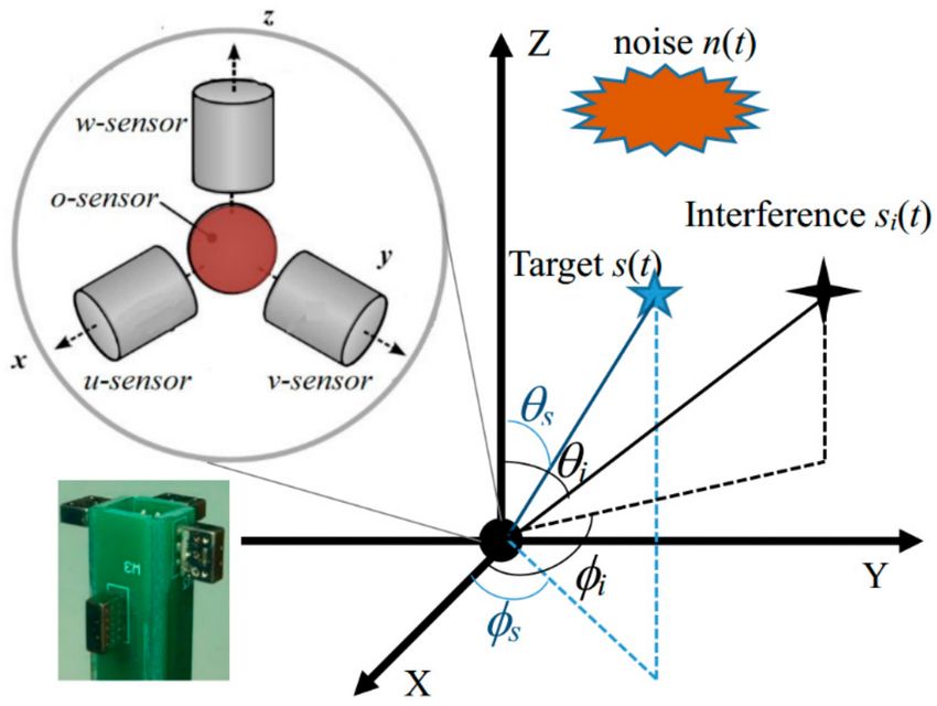
Appl. Sci. 2018, 8, 1436                                                                            2 of 17

behind mask-based SE methods is to estimate a spectrographic binary or soft mask to suppress the
unwanted spectrogram components [7–11]. For binary mask-based SE methods, the spectrographic
masks are “hard binary masks” where a spectral component is either set to 1 for the target speech
component or set to 0 for the non-target speech component. Experimental results have shown that
the performance of binary mask SE methods degrades with the decrease of the signal-to-noise ratio
(SNR) and the masked spectral may cause the loss of speech components due to the harsh black or
white binary conditions [7,8]. To overcome this disadvantage, the soft mask-based SE methods have
been developed [8]. In soft mask-based SE methods, each time-frequency component is assigned a
probability linked to the target speech. Compared to the binary mask SE methods, the soft-mask SE
methods have shown better capability to suppress the noise with the aid of some priori information.
However, the priori information may vary with time, and obtaining the priori information is not an
easy task.
     By further analyzing the mask-based SE algorithms, we have the following observations. (1) It is
a challenging task to estimate a good binary spectrographic mask. When noise and competing
speakers (speech interferences) exist, the speech enhanced by the estimated mask often suffers from the
phenomenon of “musical noise”. (2) The direction of arrival (DOA) of the target speech is considered
as a known parameter for the target SE task. (3) A binaural microphone and an acoustic vector sensor
(AVS) are considered as the most attractive front ends for speech applications due to their small
physical size. For the AVS, its physical size is about 1–2 cm3 and AVS also has the merits such as signal
time alignment and a trigonometric relationship of signal amplitudes [12–16]. A high-resolution DOA
estimation algorithm with a single AVS has been proposed by our team [12–16]. Some effort has also
been made for the target SE task with one or two AVS sensors [17–21]. For example, with the minimum
variance distortionless response (MVDR) criterion, Lockwood et al. developed a beamforming method
using the AVS [17]. Their experimental results showed that their proposed algorithm achieves good
performance for suppressing noise, but brings certain distortion of the target speech.
     As discussed above, in this study, we focus on developing the target speech enhancement
algorithm with a single AVS from a new technical perspective in which both the ambient noise and
non-target spatial speech interferences can be suppressed effectively and simultaneously. The problem
formulation is presented in Section 2. Section 3 shows the derivation of the proposed SE algorithm.
The experimental results are given in Section 4, and conclusions are drawn in Section 5.

2. Problem Formulation
     In this section, the sparsity of speech in the time-frequency (TF) domain is discussed first. Then,
the AVS data model and the corresponding inter-sensor data ratio (ISDR) models are presented for
completeness, which was developed by our team in a previous work [13]. After that, the derivation
of monotone functions between ISDRs and the DOA is given. Finally, the nonlinear soft TF mask
estimation algorithm is derived specifically.

2.1. Time-Frequency Sparsity of Speech
     In the research of speech signal processing, the TF sparsity of speech is a widely accepted
assumption. More specifically, when there is more than one speaker in the same spatial space,
the speech TF sparsity implies the following [5]. (1) It is likely that only one speaker is active during
certain time slots. (2) For the same time slot, if more than one speaker is active, it is probable that
the different TF points are dominated by different speakers. Hence, the TF sparsity of speech can be
modeled as:
                                    Sm (τ, ω )Sn (τ, ω ) = 0, m 6= n                                   (1)

where Sm (τ,ω) and Sn (τ,ω) are the speech spectral at (τ,ω) for the mth speaker and nth speaker,
respectively. (3) In practice, at a specific TF point (τ,ω), it is most probably true that only one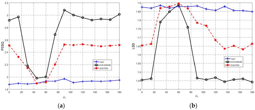
Appl. Sci. 2018, 8, 1436 3 of 17
speech source with the highest energy dominates, and the contributions from the other sources can
be negligible.
2.2. AVS Data Model
An AVS unit generally consists of J co-located constituent sensors, including one omnidirectional
sensor (denoted as o-sensor) and J-1 orthogonally oriented directional sensors. Figure 1 shows the data
capture setup with a single AVS. It is noted that the left bottom plot in Figure 1 shows a 3D-AVS unit
implemented by our team, which consists of one o-sensor with three orthogonally oriented directional
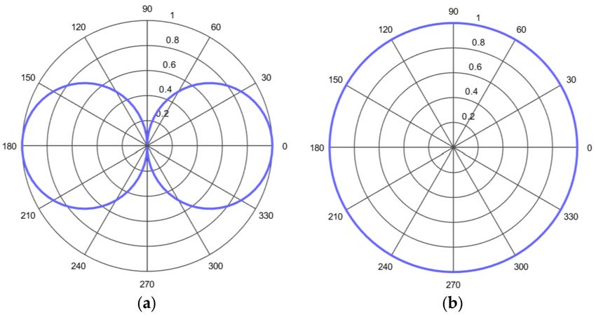
sensors depicted as the u-sensor, v-sensor, and w-sensor, respectively. In theory, the directional
response of the oriented directional sensor has dipole characteristics, as shown in Figure 2a, while the
omnidirectional sensor has the same response in all of the directions, as shown in Figure 2b. In this
study, one target speaker is considered. As shown in Figure 1, the target speech S(t) is impinging from
(θ s ,φs ) meanwhile, interference Si (t) are impinging from (θ j ,φj ), where φs , φi (0◦ ,360◦ ) are the azimuth
angles, and θ s , θ i (0◦ ,180◦ ) are the elevation angles.
Figure 1. Illustration of a single acoustic vector sensor (AVS) for data capturing.
Figure 2. (a) The directional response of oriented directional sensor; (b) The directional response of
omnidirectional sensor.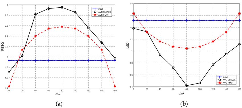
Appl. Sci. 2018, 8, 1436                                                                                           4 of 17

    For simplifying the derivation, without considering room reverberation, the received data of the
AVS can be modeled as [13]:

                                                                     Mi
                                    xavs (t) = a(θs , φs )s(t) + ∑ a(θi , φi )si (t) + navs (t)                       (2)
                                                                     i =1

where xavs (t), navs (t) and a(θ s ,φs ) are defined respectively as:

                                              xavs (t) = [ xu (t), xv (t), xw (t), xo (t)]                            (3)

                                              navs (t) = [nu (t), nv (t), nw (t), no (t)]                             (4)
                                                           T                                                   T
                           a(θs , φs ) = [us , vs , ws , 1] = [sin θs cos φs , sin θs sin φs , cos θs , 1]            (5)
                                                           T                                                   T
                             a(θi , φi ) = [ui , vi , wi , 1] = [sin θi cos φi , sin θi sin φi , cos θi , 1]          (6)

     In Equation (3), xu (t), xv (t), xw (t), xo (t) are the received data of the u-sensor, v-sensor, w-sensor,
and o-sensor, respectively; nu (t), nv (t), nw (t), no (t) are assumed as the additive zero-mean white
Gaussian noise captured at the u-sensor, v-sensor, w-sensor, and o-sensor, respectively; s(t) is the target
speech; si (t) are the ith interfering speech; the number of interferences is Mi ; a(θ s ,φs ) and a(θ j ,φj ) are
the steering vectors of s(t) and si (t), respectively. [.]T denotes the vector/matrix transposition.
     From the AVS data model given in Equation (2), taking the short-time Fourier transform (STFT),
for a specific TF point (τ,ω), we have:

                                                                     Mi
                           X avs (τ, ω ) = a(θs , φs )S(τ, ω ) + ∑ a(θi , φi )Si (τ, ω ) + N avs (τ, ω )              (7)
                                                                     i =1

where X avs (τ,ω) = [Xu (τ,ω), Xv (τ,ω), Xw (τ,ω), Xo (τ,ω)]T ; Xu (τ,ω), Xv (τ,ω), Xw (τ,ω), and Xo (τ,ω)
are the STFT of xu (t), xv (t), xw (t), and xo (t), respectively. Meanwhile, N avs (τ,ω) = [Nu (τ,ω), Nv (τ,ω),
Nw (τ,ω), No (τ,ω)]T ; Nu (τ,ω), Nv (τ,ω), Nw (τ,ω), and No (τ,ω) are the STFT of nu (t), nv (t), nw (t), and no (t),
respectively. Since the target speech spectral is S(τ,ω), let us define a quantity as follows:

                                                          Mi
                                      N total (τ, ω ) =   ∑ a(θi , φi )Si (τ, ω ) + N avs (τ, ω )                     (8)
                                                          i =1

where we define N total (τ,ω) = [Ntu (τ,ω), Ntv (τ,ω), Ntw (τ,ω), Nto (τ,ω)]T to represent the mixture of the
interferences and additive noise. Therefore, from Equations (7) and (8), we have the following expressions:

                                              Xu (τ, ω ) = us S(τ, ω ) + Ntu (τ, ω )                                  (9)

                                               Xv (τ, ω ) = vs S(τ, ω ) + Ntv (τ, ω )                               (10)

                                              Xw (τ, ω ) = ws S(τ, ω ) + Ntw (τ, ω )                                (11)

                                                Xo (τ, ω ) = S(τ, ω ) + Nto (τ, ω )                                 (12)

     In this study, we make the following assumptions. (1) s(t) and si (t) are uncorrelated and are
considered as far-field speech sources; (2) nu (t), nv (t), nw (t) and no (t) are uncorrelated. (3) The DOA of
the target speaker is given as (θ s ,φs ); the task of target speech enhancement is essentially to estimate
S(τ,ω) from X avs (τ,ω).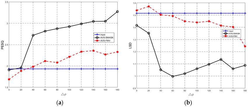
Appl. Sci. 2018, 8, 1436                                                                                   5 of 17

2.3. Monotone Functions between ISDRs and the DOA
     Definition and some discussions on the inter-sensor data ratio (ISDR) of the AVS are presented in
our previous work [13]. In this subsection, we briefly introduce the definition of ISDR first, and then
present the derivation of the monotone functions between the ISDRs and the DOA of the target speaker.
     The ISDRs between each channel of the AVS are defined as:

                                      Iij (τ, ω ) = Xi (τ, ω )/X j (τ, ω ) where (i 6= j)                   (13)

where i and j are the channel index, which refers to u, v, w, and o, respectively. Obviously, there are
12 different computable ISDRs, which are shown in Table 1. In the following context, we carefully
evaluate Iij , and it is clear that only three ISDRs (Iuv , Ivu and Iwo ) hold the approximate monotone
function between ISDR and the DOA of the target speaker.

                               Table 1. Twelve computable inter-sensor data ratios (ISDRs).

                               Sensor           u             v             w               o
                                  u           NULL           Ivu           Iwu           Iou
                                  v            Iuv          NULL           Iwv           Iov
                                  w            Iuw           Ivw          NULL           Iow
                                  o            Iuo           Ivo           Iwo          NULL

    According to the definition of ISDRs given in Equation (13), we look at Iuv , Ivu and Iwo first.
Specifically, we have:
                                 Iuv (τ, ω ) = Xu (τ, ω )/Xv (τ, ω )                           (14)

                                             Ivu (τ, ω ) = Xv (τ, ω )/Xu (τ, ω )                            (15)

                                             Iwo (τ, ω ) = Xw (τ, ω )/Xo (τ, ω )                            (16)

      Substituting Equations (9) and (10) into Equation (14) gives:

                              us S(τ, ω ) + Ntu (τ, ω )   us + Ntu (τ, ω )/S(τ, ω )   us + ε tus (τ, ω )
              Iuv (τ, ω ) =                             =                           =                       (17)
                              vs S(τ, ω ) + Ntv (τ, ω )   vs + Ntv (τ, ω )/S(τ, ω )   vs + ε tvs (τ, ω )

where εtus (τ,ω) = Ntu (τ,ω)/S(τ,ω), and εtvs (τ,ω) = Ntv (τ,ω)/S(τ,ω).
    Similarly, we get Iuw and Iwo :

                              vs S(τ, ω ) + Ntv (τ, ω )   vs + Ntv (τ, ω )/S(τ, ω )   vs + ε tvs (τ, ω )
             Ivu (τ, ω ) =                              =                           =                       (18)
                              us S(τ, ω ) + Ntu (τ, ω )   us + Ntu (τ, ω )/S(τ, ω )   us + ε tus (τ, ω )

                              ws S(τ, ω ) + Ntw (τ, ω )   ws + Ntw (τ, ω )/S(τ, ω )   ws + ε tws (τ, ω )
            Iwo (τ, ω ) =                               =                           =                       (19)
                               S(τ, ω ) + Nto (τ, ω )      1 + Nto (τ, ω )/S(τ, ω )    1 + ε tos (τ, ω )
     In Equation (19), εtws (τ,ω) = Ntw (τ,ω)/S(τ,ω) and εtos (τ,ω) = Nto (τ,ω)/S (τ,ω).
     Based on the assumption of TF sparsity of speech shown in Section 2.1, we can see that if the TF
points (τ,ω) are dominated by the target speech from (θ s ,φs ), the energy of the target speech is high,
and the value of εtus (τ,ω), εtvs (τ,ω), εtws (τ,ω) and εtos (τ,ω) tends to be small. Then, Equations (17)–(19)
can be accordingly approximated as:

                                              Iuv (τ, ω ) ≈ us /vs + ε 1 (τ, ω )                            (20)

                                              Ivu (τ, ω ) ≈ vs /us + ε 2 (τ, ω )                            (21)

                                                Iwo (τ, ω ) ≈ ws + ε 3 (τ, ω )                              (22)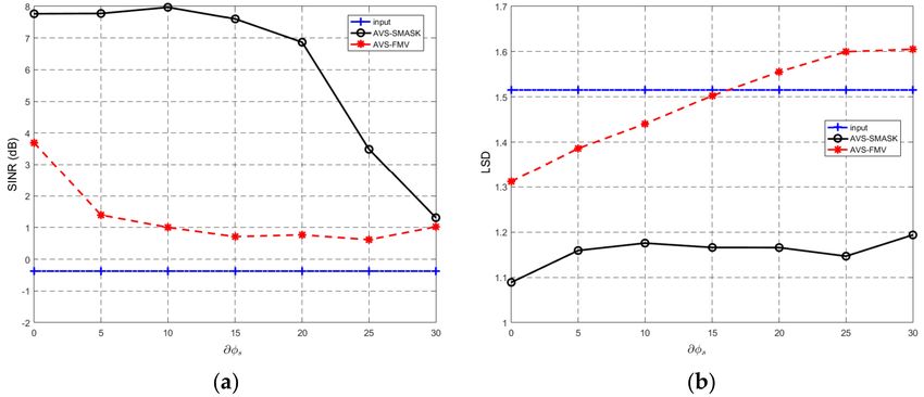
Appl. Sci. 2018, 8, 1436                                                                                              6 of 17

where ε1 , ε2 , and ε3 can be viewed as the ISDR modeling error with zero-mean introduced by
interferences and background noise. Moreover, εi (τ,ω) (i = 1, 2, 3) is inversely proportion to the
local SNR at (τ,ω).
     Furthermore, from Equation (5), we have us = sinθ s ·cosφs , vs = sinθ s ·sinφs and ws = cosθ s . Then,
substituting Equation (5) into Equations (20)–(22), we obtain the following equations:

                                                sin θs cos φs
                               Iuv (τ, ω ) ≈                  + ε 1 (τ, ω ) = cot φs + ε 1 (τ, ω )                     (23)
                                                sin θs sin φs

                                               sin θs sin φs
                              Ivu (τ, ω ) ≈                  + ε 2 (τ, ω ) = tan(φs ) + ε 2 (τ, ω )                    (24)
                                               sin θs cos φs
                                    Iwo (τ, ω ) ≈ ws + ε 3 (τ, ω ) = cos(θs ) + ε 3 (τ, ω )                            (25)

       From Equations (23)–(25), it is desired to see that the approximate monotone functions between
Iuv , Ivu , and Iwo and the DOA (θ s or φs ) of the target speaker have been obtained since arccot, arctan,
and arccos functions are all monotone functions.
       However, except for Iuv , Ivu , and Iwo , other ISDRs do not hold such a property. Let’s take Iuw as an
example. From the definition in Equation (13), we can get:

                      us S(τ, ω ) + Ntu (τ, ω )   us + Ntu (τ, ω )/S(τ, ω )   us + ε tus (τ, ω )   us
      Iuw (τ, ω ) =                             =                           =                    =    + ε 4 (τ, ω )    (26)
                      ws S(τ, ω ) + Ntw (τ, ω )   ws + Ntw (τ, ω )/S(τ, ω )   ws + ε tws (τ, ω )   ws

where ε4 can be viewed as the ISDR modeling error with zero-mean introduced by unwanted noise.
Obviously, Equation (26) is valid when ws is not equal to zero. Substituting Equation (5) into
Equation (26) yields:

                                            sin θs cos φs
                            Iuw (τ, ω ) ≈                 + ε 4 (τ, ω ) = tan θs cos φs + ε 4 (τ, ω )                  (27)
                                               cos θs

     From Equation (27), we can see that Iuw is a function of both θ s and φs .
     In summary, after analyzing all of the ISDRs, we find that the desired monotone functions
between ISDRs and θ s or φs , which are given in Equations (23)–(25), respectively. It is noted that
Equations (23)–(25) are derived conditioned by assuming vs , us , and ws are not equal to zero. Therefore,
we need to find out where vs , us , and ws are equal to zero. For presentation clarity, let’s define an ISDR
vector Iisdr = [Iuv , Ivu , Iwo ].
     From Equation (5), it is clear that when the target speaker is at angles of 0◦ , 90◦ , 180◦ , and 270◦ ,
one of vs , us , and ws becomes zero, and it means that Iisdr is not fully available. Specifically, we need to
consider the following cases:
     Case 1: the elevation angle θ s is about 0◦ or 180◦ . In this case, us = sinθ s ·cosφs and vs = sinθ s ·sinφs
are close to zero. Then, the denominator in Equations (20) and (21) is equal to zero, and we cannot
obtain Iuv and Ivu , but we can get Iwo .
     Case 2: θ s is away from 0◦ or 180◦ . In this condition, we need to look at φs carefully.

(1)     φs is about 0◦ or 180◦ . Then, vs = sinθ s sinφs is close to zero, and the denominator in Equation (20)
        is equal to zero, which leads to Iuv being invalid. In this case, we can compute Ivu and Iwo properly.
(2)     φs is about 90◦ or 270◦ . Then, us = sinθ s ·cosφs is close to zero, and the denominator in Equation (21)
        is equal to zero, which leads to Ivu being invalid. In this case, we can obtain Iuv and Iwo properly.
(3)     φs is away from 0◦ , 90◦ , 180◦ , and 270◦ , we can obtain all of the Iuv , Ivu and Iwo values properly.

      To visualize the discussions above, a decision tree of handling the special angles in computing
Iisdr is plotted in Figure 3.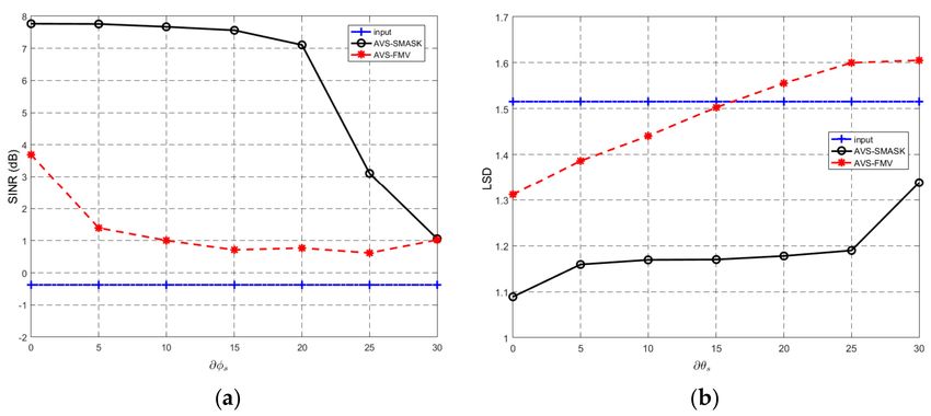
Appl. Sci. 2018, 8, 1436                                                                                        7 of 17

                     Figure 3. The decision tree of handling the special angles in computing Iisdr .

    When Iisdr = [Iuv , Ivu , Iwo ] has been computed properly, with simple manipulation from
Equations (23)–(25), we get:

                                      φs (τ, ω ) = arccot( Iuv (τ, ω ) − ε 1 (τ, ω ))                            (28)

                                      φs (τ, ω ) = arctan( Ivu (τ, ω ) − ε 2 (τ, ω ))                            (29)

                                      θs (τ, ω ) = arccos( Iwo (τ, ω ) − ε 3 (τ, ω ))                            (30)

     From Equations (28)–(30), we can see that arccot, arctan, and arccos functions are all monotone
functions, which are what we expected. Besides, we also note that (θ s ,φs ) is given, and Iuv , Ivu and
Iwo can be computed by Equations (14)–(16). However, ε1 , ε2 , and ε3 are unknown, which reflect the
impact of noise and interferences. According to the assumptions made in Section 2.1, if we are able
to select the TF components (θ s ,φs ) dominated by the target speech, and the local SNR at this (τ,ω) is
high, then ε1 , ε2 , and ε3 can be ignored, since they will have values approaching zero at these (τ,ω)
points. In such conditions, we obtain the desired formulas to compute (θ s ,φs ):

     φs (τ, ω ) ≈ arccot( Iuv (τ, ω )), φs (τ, ω ) ≈ arctan( Ivu (τ, ω ))andθs (τ, ω ) ≈ arccos( Iwo (τ, ω ))    (31)

2.4. Nonlinear Soft Time-Frequency (TF) Mask Estimation
     As discussed above, Equation (31) is valid when the (τ,ω) points are dominated by target speech
with high local SNR. Besides, we have three equations to solve two variables, θ s and φs . In this study,
from Equation (31), we estimate θ s and φs in the following way:

                                         φ̂s1 (τ, ω ) = arccotIuv (τ, ω ) + ∆η1                                  (32)

                                         φ̂s2 (τ, ω ) = arctanIvu (τ, ω ) + ∆η2                                  (33)

                                              φ̂s (τ, ω ) = mean(φ̂s1 , φ̂s2 )                                   (34)

                                         θ̂s (τ, ω ) = arccosIwo (τ, ω ) + ∆η3                                   (35)

where ∆η 1 and ∆η 2 are estimation errors. Comparing Equation (31) and Equations (32)–(35), we can
see that if the estimated DOA values (φ̂s (τ, ω ),θ̂s (τ, ω )) approximate to the real DOA values (θ s ,φs ),
then ∆η 1 and ∆η 2 should be small. Therefore, for the TF points (τ,ω) dominated by the target speech,
we can derive the following inequality:

                                                  φ̂s (τ, ω ) − φs < δ1                                          (36)

                                                   θ̂s (τ, ω ) − θs < δ2                                         (37)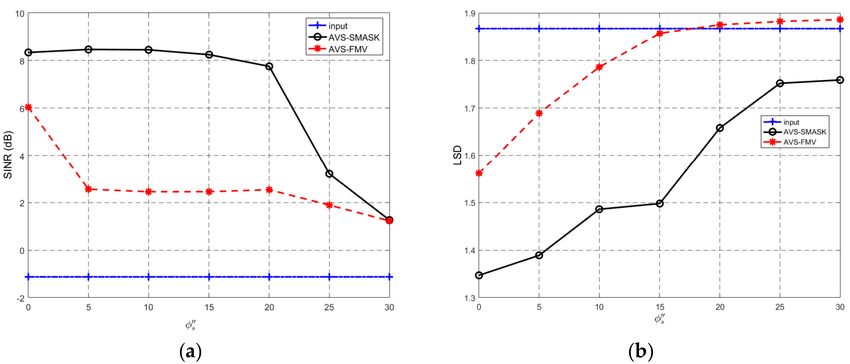
Appl. Sci. 2018, 8, 1436 8 of 17
where φ̂s (τ, ω ) and θ̂s (τ, ω ) are the target speaker’s DOA estimated by Equations (34) and (35),
respectively. θ s and φs are given the DOA of the target speech for the SE task. The parameters δ1 and
δ2 can be set as the predefined permissible parameters (referring to an angle value). Following the
derivation up to now, if Equations (36) and (37) are met at (τ,ω) points, we can infer that these (τ,ω)
points are dominated by the target speech with high probability. Therefore, using Equations (36) and
(37), the TF points (τ,ω) can be extracted, and a mask associated with these (τ,ω) points dominated by
the target speech can be designed accordingly. In addition, we need to take the following facts into
account. (1) The value of φs belongs to (0,2π]. (2) The principal value interval of the arccot function
is (0,π), and the arctan function is (−π/2,π/2). (3) The value range of θ s is (0,2π]. (4) The principal
value interval of the arccos function is [0,π]. (5) To make the principal value of the anti-trigonometric
function match the value of θ s and φs , we need to add Lπ to avoid ambiguity. As a result, a binary TF
mask for preserving the target speech is designed as follows:
(
1, if ∆φ(τ, ω ) = φ̂s (τ, ω ) − φs + Lπ < δ1
mask (τ, ω ) = ∆θ (τ, ω ) = θ̂s (τ, ω ) − θs + Lπ < δ2 (38)
0, else
where L = 0, ± 1. (∆φ(τ,ω), ∆θ(τ,ω)) is the estimation difference between the estimated DOA and
the real DOA of the target speaker at TF point (τ,ω). Obviously, the smaller the value of (∆φ(τ,ω),
∆θ(τ,ω)), the more probable it is that the TF point (τ,ω) is dominated by the target speech. To further
improve the estimation accuracy and suppress the impact of the outliers, we propose a nonlinear soft
TF mask as: (
1
∆φ < δ1 & ∆θ < δ2
mask (τ, ω ) = 1+e−ξ (1−(∆φ(τ,ω )/δ1 +∆θ (τ,ω )/δ2 )/2) (39)
ρ else
where ξ is a positive parameter and ρ (0 ≤ ρ < 1) is a small positive parameter tending to be zero,
which reflects the noise suppression effect. The parameters ∆1 and ∆2 control the degree of the
estimation difference (∆φ(τ,ω), ∆θ(τ,ω). When parameters ∆1 , ∆2 , and ρ become larger, the capability
of suppressing noise and interferences degrades, and the possibility of the (τ,ω) being dominated by
the target speech also degrades. Hence, selecting the values of ρ, ∆1 , and ∆2 is important. In our study,
these parameters are determined through experiments. Future work could focus on selecting these
parameters based on models of human auditory perception. In the end, we need to emphasize that the
mask designed in Equation (39) has the ability to suppress the adverse effects of the interferences and
background noise, and preserve the target speech simultaneously.
3. Proposed Target Speech Enhancement Method
The diagram of the proposed speech enhancement method (termed as AVS-SMASK) is shown in
Figure 4, which is processed in the time-frequency domain. The details of each block in Figure 4 will
be addressed in the following context.
Figure 4. Block diagram of our proposed AVS-SMASK algorithm (STFT: Short-Time Fourier Transform;
FBF: a fixed beamformer; ISTFT: inverse STFT; y(n): enhanced target speech).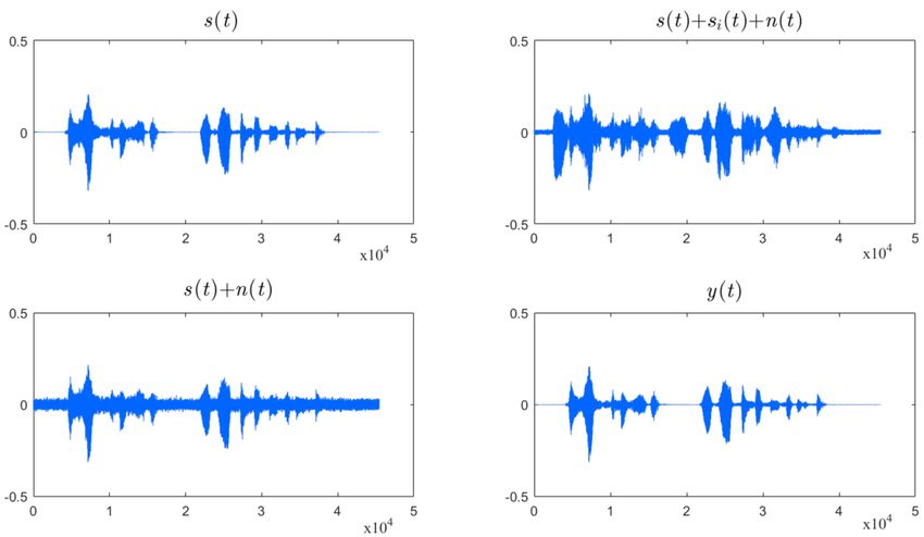
Appl. Sci. 2018, 8, 1436                                                                                            9 of 17

3.1. The FBF Spatial Filter
     As shown in Figure 4, the input signals to the FBF spatial filter are the data captured by the u, v,
and w-sensor of the AVS. With the given DOA (θ s ,φs ), the spatial matched filter (SMF) is employed as
the FBF spatial filter, and its output can be described as:

                                                              H
                                                Ym (τ, ω ) = wm Xavs (τ, ω )                                         (40)

where wm H = aH (θ s ,φs )/||a(θ s ,φs ) ||2 is the weight vector of the SMF, and a(θ s ,φs ) is given in
Equation (5). [.]H denotes the vector/matrix conjugate transposition. Substituting the expressions in
Equations (5), (3), and (9)–(11) in Equation (40) yields:

   Ym (τ, ω )     = us Xu (τ, ω ) + vs Xv (τ, ω ) + ws Xw (τ, ω )
                  = u2s S(τ, ω ) + us Ntu (τ, ω ) + v2s S(τ, ω ) + vs Ntv (τ, ω ) + w2s S(τ, ω ) + ws Ntw (τ, ω )
                                                                                                                     (41)
                  = (u2s + v2s + w2s )S(τ, ω ) + Ntuvw (τ, ω )
                  = S(τ, ω ) + Ntuvw (τ, ω )

where Ntuvw (τ,ω) is the total noise component given as:

       Ntuvw (τ, ω )       = us Ntu (τ, ω ) + vs Ntv (τ, ω ) + ws Ntw (τ, ω )
                           = us (ui Si (τ, ω ) + Nu (τ, ω )) + vs (vi Si (τ, ω ) + Nv (τ, ω ))
                                                                                                                     (42)
                             +ws (wi Si (τ, ω ) + Nw (τ, ω ))
                           = (us ui + vs vi + ws wi )Si (τ, ω ) + us Nu (τ, ω ) + vs Nv (τ, ω ) + ws Nw (τ, ω )

     It can been seen that Ntuvw (τ,ω) in Equation (42) consists of the interferences and background
noise captured by directional sensors, while Ym (τ,ω) in Equation (41) is the mix of the desired speech
source S(τ,ω) and unwanted component Ntuvw (τ,ω).

3.2. Enhancing Target Speech Using Estimated Mask
    With the estimated mask in Equation (39) and the output of the FBF spatial filter Ym (τ,ω) in
Equation (42), it is straightforward to compute the enhanced target speech as follows:

                                            Ys (τ, ω ) = Ym (τ, ω ) × mask(τ, ω )                                    (43)

where Ys (τ,ω) is then the spectra of the enhanced speech or an approximation of the target speech.
    For presentation completeness, our proposed speech enhancement algorithm is termed as an
AVS-SMASK algorithm, which is summarized in Table 2.

                            Table 2. The pseudo-code of our proposed AVS-SMASK algorithm.

 (1)  Segment the output data captured by the u-sensor, v-sensor, w-sensor, and o-sensor of the AVS unit by the
      N-length Hamming window;
 (2) Calculate the STFT of the segments: Xu (τ,ω), Xv (τ,ω), Xw (τ,ω) and Xo (τ,ω);
 (3) Calculate the ISDR vector Iisdr = [Iuv , Ivu , Iwo ] by Equations (14)–(16);
 (4) Obtain the valid Iisdr according to the known direction of arrival (DOA) (θ s ,φs ) and the summary of
      Section 2.3;
 (5) Utilize the valid Iisdr to estimate the DOA (θ̂s ,φ̂s ) of the target speech for each time-frequency (TF) point;
 (6) Determine TF points belong to the target speech by Equations (36) and (37);
 (7) Calculate the nonlinear soft TF mask: mask(τ,ω) by Equation (39);
 (8) Calculate the output of the FBF Ym (τ,ω) by Equation (40);
 (9) Compute the enhanced speech spectrogram by Equation (43);
 (10) Get the enhanced speech signal y(n) by ISTFT.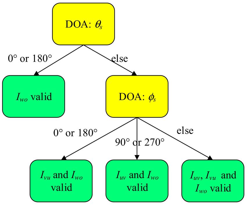
Appl. Sci. 2018, 8, 1436                                                                                  10 of 17

4. Experiments and Results
     The performance evaluation of our proposed AVS-SMASK algorithm has been carried out with
simulated data and recorded data. Five commonly used performance measurement metrics—SNR,
the signal-to-interference ratio (SIR), the signal-to-interference plus noise ratio (SINR), log spectral
division (LSD), and the perceptual evaluation of speech quality (PESQ)—have been adopted.
The definitions are given as follows for presentation completeness.

(1)    Signal-to-Noise Ratio (SNR):

                                         SNR = 10 log ks(t)k2 /kn(t)k2                                         (44)

(2)    Signal-to-Interference Ratio (SIR)

                                         SIR = 10 log ks(t)k2 /ksi (t)k2                                       (45)

(3)    Signal-to-Interference plus Noise Ratio (SINR):

                                     SI NR = 10 log ks(t)k2 /k x (t) − s(t)k2                                  (46)

       where s(t) is the target speech, n(t) is the additive noise, si (t) is the ith interference,
       and x(t) = s(t) + si (t) + n(t) is the received signal of the o-sensor. The metrics are calculated
       by averaging over frames to get more accurate measurement [22].
(4)    Log Spectral Deviation (LSD), which is used to measure the speech distortion [22]:

                                            LSD = kln ψss ( f )/ψyy ( f ) k                                    (47)

       where ψss ( f ) is the power spectral density (PSD) of the target speech, and ψyy ( f ) is the PSD of
       the enhanced speech. It is clear that smaller LSD values indicate less speech distortion.
(5)    Perceptual Evaluation of Speech Quality (PESQ). To evaluate the perceptual enhancement
       performance of the speech enhancement algorithms, the ITU-PESQ software [23] is utilized.

      In this study, the performance comparison is carried out with the comparison algorithm
AVS-FMV [17] under the same conditions. We do not take other SE methods into account since
they use different transducers for signal acquisition. One set of waveform examples that is used in our
experiments is shown in Figure 5, where s(t) is the target speech, si (t) is the i-th interference speech,
n(t) is the additive noise, and y(t) is the enhanced speech.

      Figure 5. Waveform examples: s(t) is the target speech, si (t) is the interference speech, n(t) is the
      additive noise, and y(t) is the enhanced speech signal.
Appl. Sci. 2018, 8, 1436 11 of 17
4.1. Experiments on Simulated Data
In this section, three experiments have been carried out. The simulated data of about five seconds
duration is generated, where the target speech s(t) is male speech, and two speech interferences
si (t) are male and female speech, respectively. Moreover, the AURORA2 database [24] was used,
which includes subway, babble, car, exhibition noise, etc. Without loss of generality, all of the speech
sources are placed one meter away from the AVS.
4.1.1. Experiment 1: The Output SINR Performance under Different Noise Conditions
In this experiment, we have carried out 12 trials (numbered as trial 1 to trial 12) to evaluate the
performance of the algorithms under different spatial and additive noise conditions following the
experimental protocols in Ref. [25]. The details are given below:
(1) The DOAs of target speech, the first speech interference (male speech) and the second speech
interference (female speech) are at (θ s ,φs ) = (45◦ ,45◦ ), (θ 1 ,φ1 ) = (90◦ ,135◦ ), and (θ 2 ,φ2 ) = (45◦ ,120◦ ),
respectively. The background noise is chosen as babble noise n(t);
(2) We evaluate the performance under three different conditions: (a) there exists only additive
background noise: n(t) 6= 0 and si (t) = 0; (b) there exists only speech interferences: n(t) = 0 and si (t) 6= 0;
(c) there exists both background noise and speech interferences: n(t) 6= 0 and si (t) 6= 0;
(3) The input SINR (denoted as SINR-input) is set as −5 dB, 0 dB, 5 dB, and 10 dB, respectively.
Following the setting above, 12 different datasets are generated for this experiment.
In addition, the parameters of algorithms are set as follows. (1) The sampling rate is 16 kHz,
1024-point FFT (Fast Fourier Fransform), and 1024-point Hamming window with 50% overlapping
are used. (2) For our proposed AVS-SMASK algorithm, we set δ1 = δ2 = 25◦ , ρ = 0.07, and ξ = 3.
(3) For comparing algorithm AVS-FMV: F = 32, M = 1.001 followed Ref. [17]. The experimental results
are given in Table 3.
Table 3. Output signal-to-interference plus noise ratio (SINR) under different noise conditions.
AVS-FMV [17] (dB) AVS-SMASK (dB)
Noise Conditions SINR-Input (dB)
SINR-Out Average SINR-Out Average
Trial 1 (n(t) = 0 and si (t) 6= 0 ) −5 4.96 7.32
Trial 2 (n(t) = 0 and si (t) 6= 0 ) 0 5.60 9.38
4.88 8.14
Trial 3 (n(t)= 0 and si (t) 6= 0 ) 5 7.81 11.53
Trial 4 (n(t)= 0 and si (t) 6= 0 ) 10 11.15 14.31
Trial 5 (n(t) 6= 0 and si (t) = 0 ) −5 4.77 6.70
Trial 6 (n(t) 6= 0 and si (t) = 0 ) 0 5.51 10.17
4.97 9.11
Trial 7 (n(t) 6= 0 and si (t) = 0 ) 5 6.76 13.03
Trial 8 (n(t) 6= 0 and si (t) = 0 ) 10 12.83 16.55
Trial 9 (n(t) 6= 0 and si (t) 6= 0 ) −5 3.66 4.70
Trial 10 (n(t) 6= 0 and si (t) 6= 0 ) 0 5.70 7.22
4.42 6.66
Trial 11 (n(t) 6= 0 and si (t) 6= 0 ) 5 7.10 10.46
Trial 12 (n(t) 6= 0 and si (t) 6= 0 ) 10 11.20 14.27
As shown in Table 3, for all of the noise conditions (Trial 1 to Trial 12), our proposed AVS-SMASK
algorithm outperforms AVS-FMV [17]. From Table 3, we can see that our proposed AVS-SMASK
algorithm gives about 3.26 dB, 4.14 dB, and 2.25 dB improvement compared with that of AVS-FMV
under three different experimental settings, respectively. We can conclude that our proposed
AVS-SMASK is effective in suppressing the spatial interferences and background noise.
4.1.2. Experiment 2: The Performance versus Angle Difference
This experiment evaluates the performance of SE methods versus the angle difference between
the target and interference speakers. Let’s define the angle difference as ∆φ= φs − φI and ∆θ = θ − θ iAppl. Sci. 2018, 8, 1436 12 of 17
(here, the subscripts s and i refer to the target speaker and the interference speaker, respectively).
Obviously, the closer the interference speaker is to the target speaker, the speech enhancement is
more limited. The experimental settings are as follows. (1) PESQ and LSD are used as metrics.
(2) The parameters of algorithms are set as the same as those used in Experiment 1. (3) Without loss of
generality, the SIR-input is set 0 dB, while SNR-input is set 10 dB. (4) We consider two cases.
• Case 1: ∆θ is fixed and ∆φ is varied, (θ 1 ,φ1 ) = (45◦ ,0◦ ), the DOA of the target speaker moves from
(θ s ,φs ) = (45◦ ,0◦ ) to (θ s ,φs ) (45◦ ,180◦ ) with 20◦ increments. Hence, the angle difference ∆φ changes
from 0◦ to 180◦ with 20◦ increments. Figure 6 shows the results of Case 1. From Figure 6, it is clear
to see that when ∆φ→0◦ (the target speaker moves closer to the interference speaker), for both
algorithms, the PESQ drops significantly, and the LSD values are also big. These results indicate
that the speech enhancement is very much limited if ∆φ→0◦ . However, when ∆φ > 20◦ , the PESQ
gradually increases, and LSD drops. It is quite encouraging to see that the performance of PESQ
and LSD of our proposed AVS-SMASK algorithm is superior to that of the AVS-FMV algorithm
for all of the angles. Moreover, our proposed AVS-SMASK algorithm has the absolute advantage
when ∆φ ≥ 40◦ .
• Case 2: ∆φ is fixed and ∆θ is varied, (θ 1 ,φ1 ) = (10◦ ,75◦ ), the DOA of the target speaker moves
from (θ s ,φs ) = (10◦ ,75◦ ) to (θ s ,φs ) = (170◦ ,75◦ ) with 20◦ increments. Then, the angle difference ∆θ
changes from 0◦ to 160◦ with 20◦ increments. Figure 7 shows the results of Case 2. From Figure 7,
we can see that when ∆θ →0◦ (the target speaker moves closer to the interference speaker),
for both algorithms, the performance of PESQ and LSD are also poor. This means that the speech
enhancement is very much limited if ∆θ →0◦ . However, when ∆θ > 20◦ , it is quite encouraging to
see that the performance of PESQ and LSD of our proposed AVS-SMASK algorithm outperforms
that of the AVS-FMV algorithm for all of the angles. In addition, it is noted that the performance of
two algorithms drops again when the ∆θ > 140◦ (the target speaker moves closer to the interference
speaker around a cone). However, from Figure 6, this phenomenon does not exit.
Figure 6. (Experiment 2) The perfomance versus ∆φ. (a) Perceptual evaluation of speech quality (PESQ)
results and (b) Log spectral division (LSD) results (Case 1: φs of the target speaker changes from
0◦ to 180◦ ) (Case 1).
In summary, from the experimental results, it is clear that our proposed AVS-SMASK algorithm is
able to enhance the target speech and suppress the interferences when the angle difference between
the target speaker and the interference is larger than 20◦ .Appl. Sci. 2018, 8, 1436 13 of 17
Figure 7. (Experiment 2) The performance versus ∆θ. (a) PESQ results and (b) LSD results (Case 2:
θ s of the target speaker changes from 0◦ to 160◦ ).
4.1.3. Experiment 3: The Performance versus DOA Mismatch
In practice, the DOA estimation of the target speaker may be inaccurate or the target speaker
may make a small movement that causes the DOA mismatch problem. Hence, this experiment
evaluates the impact of the DOA mismatch on the performance of our proposed speech enhancement
algorithm. The experimental settings are as follows. (1) The parameters of algorithms are set as same
as the Experiment 1. (2) (θ s ,φs ) = (45◦ ,45◦ ) and (θ 1 ,φ1 ) = (90◦ ,135◦ ). (3) The SIR-input is set to 0 dB,
while the SNR-input is set to 10 dB; the performance measurement metrics are chosen as SINR and
LSD. (4) We consider two cases:
Case 1: Only φs is mismatched, and the mismatch (∂φs ) ranges from 0◦ to 30◦ with 5◦ increments.
Case 2: Only θ s is mismatched, and the mismatch (∂θ s ) ranges from 0◦ to 30◦ with 5◦ increments.
Experimental results are given in Figures 8 and 9 for Case 1 and Case 2, respectively. From these
results, we can clearly see that when the DOA mismatch is less than 20◦ , our proposed AVS-SMASK
algorithm is not sensitive to DOA mismatch. Besides, our AVS-SMASK algorithm outperforms the
AVS-FMV algorithm under all of the conditions. However, when the DOA mismatch is larger than 20◦ ,
the performance of our proposed AVS-SMASK algorithm drops significantly. Fortunately, it is easy to
achieve 20◦ DOA estimation accuracy.
Figure 8. (Experiment 3) The performance versus the ∂φs . (a) SINR results and (b) LSD results (Case 1).Appl. Sci. 2018, 8, 1436 14 of 17
Figure 9. (Experiment 3, Case 2) The performance versus the ∂θ s . (a) SINR results and (b) LSD results
(Case 2).
4.2. Experiments on Recorded Data in an Anechoic Chamber
In this section, two experiments have been carried out with the recorded data captured by an AVS
in an anechoic chamber [25]. Every set of recordings lasts about six seconds, which is made by the
situation that the target speech source and the interference source are broadcasting at the same time
along with the background noise, as shown in Figure 1. The speech sources taken from the Institute of
Electrical and Electronic Engineers (IEEE) speech corpus [26] are placed in the front of the AVS at a
distance of one meter, and the SIR-input is set to 0 dB, while the SNR-input is set to 10 dB, and the
sampling rate was 48 kHz, and then down-sampled to 16 kHz for processing.
4.2.1. Experiment 4: The Performance versus Angle Difference with Recorded Data
In this experiment, the performance of our proposed method has been evaluated versus the
angle difference between the target and interference speakers (∆φ = φs − φi and ∆θ = θ s − θ i ).
The experimental settings are as follows. (1) PESQ is taken as the performance measurement metric.
(2) The parameters of algorithms are set as the same as that of Experiment 1. (3) Considering page
limitation, here, we only consider the changing of azimuth angle φs while θ s = 90◦ . The interfering
speaker s1 (t) is at (θ 1 ,φ1 ) = (90◦ ,45◦ ). φs varies from 0◦ to 180◦ with 20◦ increments. Then, there are
13 recorded datasets. The experimental results are shown in Figure 10. It is noted that the x-axis
represents the azimuth angle φs . It is clear to see that the overall performance of our proposed
AVS-SMASK algorithm is superior to that of the comparing algorithm. Specifically, when φs approaches
φ1 = 45◦ , the PESQ degrades quickly for both algorithms. When the angle difference ∆φ is larger than
30◦ (φs is smaller than 15◦ or larger than 75◦ ), the PESQ of our proposed AVS-SMASK algorithm goes
up quickly, and is not sensitive to the angle difference.
Figure 10. (Experiment 4) The performance versus φs . (a) PESQ results and (b) LSD results.Appl. Sci. 2018, 8, 1436 15 of 17
4.2.2. Experiment 5: Performance versus DOA Mismatch with Recorded Data
This experiment is carried out to evaluate the performance of speech enhancement algorithms
when there are DOA mismatches. The experimental settings are as follows. (1) PESQ and LSD are
taken as the performance measurement metric. (2) The parameters of algorithms are set the same as
those of Experiment 1. (3) The target speaker is at (θ s ,φs ) = (45◦ ,45◦ ), and the interference speaker is at
(θ 1 ,φ1 ) = (90◦ ,135◦ ). The azimuth angle φs is assumed to be mismatched. We consider the mismatch of
φs (denoted as φs ” ) varying from 0◦ to 30◦ with 5◦ increments. The experimental results are shown in
Figure 11, where the x-axis is the mismatch of the azimuth angle φs (φs ” ). It is noted that our proposed
AVS-SMASK is superior to the compared algorithm under all conditions. It is clear to see that our
proposed algorithm is not sensitive to DOA mismatch when the DOA mismatch is smaller than 23◦ .
Figure 11. (Experiment 5) The performance versus the φs mismatch φs ” . (a) PESQ results and
(b) LSD results.
We are encouraged to conclude that our proposed algorithm will offer a good speech enhancement
performance in practical applications when the DOA may not be accurately estimated.
5. Conclusions
In this paper, aiming at the hearing technology of service robots, a novel target speech
enhancement method has been proposed systematically with a single AVS to suppress spatial multiple
interferences and additive background noise simultaneously. By exploiting the AVS signal model and
its inter-sensor data ratio (ISDR) model, the desired monotone functions between ISDR and the DOA
of the target speaker is derived. Accordingly, a nonlinear soft mask has been designed by making use
of speech time-frequency (TF) sparsity with the known DOA of the target speaker. As a result, a single
AVS-based speech enhancement method (named as AVS-SMASK) has been formulated and evaluated.
Comparing with the existing AVS-FMV algorithm, extensive experimental results using simulated
data and recorded data validate the effectiveness of our AVS-SMASK algorithm in suppressing spatial
interferences and the additive background noise. It is encouraging to see that our AVS-SMASK
algorithm is able to maintain less speech distortion. Due to page limitations, we did not show the
derivation of the algorithm under reverberation. The signal model and ISDR model under reverberant
conditions will be presented in our paper [27]. Our preliminary experimental results show that the
PESQ of our proposed AVS-SMASK degrades gradually when the room reverberation becomes stronger
(RT60 > 400 ms), but LSD is not sensitive to the room reverberation. Besides, there is an argument that
learning-based SE methods achieve the state-of-art. In our opinion, in terms of SNR, PESQ, and LSD,
this is true. However, learning-based SE methods ask for large amounts of training data, and require
much larger memory size and a high computational cost. In contrast, the application scenarios of thisAppl. Sci. 2018, 8, 1436 16 of 17
research are different to learning-based SE methods, and our solution is more suitable for low-cost
embedded systems. A real demo system was established in our lab, and the conducted trials further
confirmed the effectiveness of our method where room reverberation is moderate (RT60 < 400 ms).
We are confident that with only four-channel sensors and without any additional training data collected,
the subjective and objective performance of our proposed AVS-SMASK is impressive. Our future study
will investigate the deep learning-based SE method with a single AVS to improve its generalization
and capability to handle different noise and interference conditions.
Author Contributions: Original draft preparation and writing, Y.Z. and Z.L.; Review & Editing, C.H.R., Y.Z. and
Z.L. carried out the studies of the DOA estimation and speech enhancement with Acoustic Vector Sensor
(AVS), participated in algorithm development, carried out experiments as well as drafted the manuscript.
C.H.R. contributed to the design of the experiments, analyzed the experimental results and helped to review and
edit the manuscript. All authors read and approved the final manuscript.
Funding: This research was funded by National Natural Science Foundation of China (No: 61271309),
Shenzhen Key Lab for Intelligent MM and VR (ZDSYS201703031405467) and the Shenzhen Science & Technology
Fundamental Research Program (JCYJ20170817160058246).
Conflicts of Interest: The authors declare no conflict of interest.
References
1. Yang, Y.; Song, H.; Liu, J. Service robot speech enhancement method using acoustic micro-sensor array.
In Proceedings of the International Conference on Advanced Intelligence and Awareness Internet (IET),
Beijing, China, 23–25 October 2010; pp. 412–415.
2. Gomez, R.; Ivanchuk, L.; Nakamura, K.; Mizumoto, T.; Nakadai, K. Utilizing visual cues in robot audition
for sound source discrimination in speech-based human-robot communication. In Proceedings of the IEEE
International Conference on Intelligent Robots and Systems, Hamburg, Germany, 28 September–2 October 2015;
pp. 4216–4222.
3. Atrash, A.; Kaplow, R.; Villemure, J.; West, R.; Yamani, H.; Pineau, J. Development and validation of a robust
speech interface for improved human-robot interaction. Int. J. Soc. Rob. 2009, 1, 345–356. [CrossRef]
4. Chen, M.; Wang, L.; Xu, C.; Li, R. A novel approach of system design for dialect speech interaction with NAO
robot. In Proceedings of the International Conference on Advanced Robotics (ICAR), Hong Kong, China,
10–12 July 2017; pp. 476–481.
5. Philipos, C.; Loizou, P.C. Speech Enhancement: Theory and Practice, 2nd ed.; CRC Press: Boca Raton, FL, USA, 2017.
6. Chen, J.; Benesty, J.; Huang, Y. New insights into the noise reduction Wiener filter. IEEE Trans. Audio Speech
Lang. Process. 2006, 14, 1218–1234. [CrossRef]
7. Reddy, A.M.; Raj, B. Soft mask methods for single-channel speaker separation. IEEE Trans. Audio Speech
Lang. Process. 2007, 15, 1766–1776. [CrossRef]
8. Lightburn, L.; De Sena, E.; Moore, A.; Naylor, P.A.; Brookes, M. Improving the perceptual quality of ideal
binary masked speech. In Proceedings of the IEEE International Conference on Acoustics, Speech and Signal
Processing (ICASSP), New Orleans, LA, USA, 5–9 March 2017; pp. 661–665.
9. Wang, Z.; Wang, D. Mask Weighted Stft Ratios for Relative Transfer Function Estimation and Its Application
to Robust ASR. In Proceedings of the IEEE International Conference on Acoustics, Speech and Signal
Processing (ICASSP), Calgary, AB, Canada, 15–20 April 2018.
10. Xiao, X.; Zhao, S.; Jones, D.L.; Chng, E.S.; Li, H. On time-frequency mask estimation for MVDR beamforming
with application in robust speech recognition. In Proceedings of the IEEE International Conference on
Acoustics, Speech and Signal Processing (ICASSP), New Orleans, LA, USA, 5–9 March 2017; pp. 3246–3250.
11. Heymann, J.; Drude, L.; Haeb-Umbach, R. Neural network based spectral mask estimation for acoustic
beamforming. In Proceedings of the IEEE International Conference on Acoustics, Speech and Signal
Processing (ICASSP), Shanghai, China, 20–25 March 2016; pp. 196–200.
12. Li, B.; Zou, Y.X. Improved DOA Estimation with Acoustic Vector Sensor Arrays Using Spatial Sparsity and
Subarray Manifold. In Proceedings of the IEEE International Conference on Acoustics, Speech and Signal
Processing (ICASSP), Kyoto, Japan, 25–30 March 2012; pp. 2557–2560.Appl. Sci. 2018, 8, 1436 17 of 17
13. Zou, Y.X.; Shi, W.; Li, B.; Ritz, C.H.; Shujau, M.; Xi, J. Multisource DOA Estimation Based On Time-Frequency
Sparsity and Joint Inter-Sensor Data Ratio with Single Acoustic Vector Sensor. In Proceedings of the IEEE
International Conference on Acoustics, Speech and Signal Processing (ICASSP), Vancouver, BC, Canada,
26–31 May 2013; pp. 4011–4015.
14. Zou, Y.X.; Guo, Y.; Zheng, W.; Ritz, C.H.; Xi, J. An effective DOA estimation by exploring the spatial sparse
representation of the inter-sensor data ratio model. In Proceedings of the IEEE China Summit & International
Conference on Signal and Information Processing (ChinaSIP), Xi’an, China, 9–13 July 2014; pp. 42–46.
15. Zou, Y.X.; Guo, Y.; Wang, Y.Q. A robust high-resolution speaker DOA estimation under reverberant
environment. In Proceedings of the International Symposium on Chinese Spoken Language
Processing (ISCSLP), Singapore, 13–16 December 2014; p. 400.
16. Zou, Y.; Gu, R.; Wang, D.; Jiang, A.; Ritz, C.H. Learning a Robust DOA Estimation Model with Acoustic
Vector Sensor Cues, In Proceedings of the Asia-Pacific Signal and Information Processing Association
(APSIPA). Kuala Lumpur, Malaysia, 12–15 December 2017.
17. Lockwood, M.E.; Jones, D.L.; Bilger, R.C.; Lansing, C.R.; O’Brien, W.D.; Wheeler, B.C.; Feng, A.S. Performance
of Time- and Frequency-domain Binaural Beamformers Based on Recorded Signals from Real Rooms.
J. Acoust. Soc. Am. 2004, 115, 379–391. [CrossRef] [PubMed]
18. Lockwood, M.E.; Jones, D.L. Beamformer Performance with Acoustic Vector Sensors in Air. J. Acoust. Soc. Am.
2006, 119, 608–619. [CrossRef] [PubMed]
19. Shujau, M.; Ritz, C.H.; Burnett, I.S. Speech Enhancement via Separation of Sources from Co-located
Microphone Recordings. In Proceedings of the IEEE International Conference on Acoustics, Speech and
Signal Processing (ICASSAP), Dallas, TX, USA, 14–19 March 2010; pp. 137–140.
20. Wu, P.K.T.; Jin, C.; Kan, A. A Multi-Microphone SPE Algorithm Tested Using Acoustic Vector Sensors.
In Proceedings of the International Workshop on Acoustic Echo and Noise Control, Tel-Aviv, Israel,
30 August–2 September 2010.
21. Zou, Y.X.; Wang, P.; Wang, Y.Q.; Ritz, C.H.; Xi, J. Speech enhancement with an acoustic vector sensor:
An effective adaptive beamforming and post-filtering approach. EURASIP J. Audio Speech Music Process 2014,
17. [CrossRef]
22. Zou, Y.X.; Wang, P.; Wang, Y.Q.; Ritz, C.H.; Xi, J. An effective target speech enhancement with single
acoustic vector sensor based on the speech time-frequency sparsity. In Proceedings of the 19th International
Conference on Digital Signal Processing (DSP), Hong Kong, China, 20–23 August 2014; pp. 547–551.
23. Gray, R.; Buzo, A.; Gray, A.; Matsuyama, Y. Distortion measures for speech processing. IEEE Trans. Acoust.
Speech Signal Process. 1980, 28, 367–376. [CrossRef]
24. ITU-T. 862-Perceptual Evaluation of Speech Quality (PESQ): An Objective Method for End-to-End Speech
Quality Assessment of Narrow-Band Telephone Networks and Speech Codecs; International Telecommunication
Union-Telecommunication Standardization Sector (ITU-T): Geneva, Switzerland, 2001.
25. Hirsch, H.G.; Pearce, D. The AURORA experimental framework for the performance evaluations of speech
recognition systems under noisy conditions. In Proceedings of the Automatic Speech Recognition: Challenges
for the Next Millennium, Paris, France, 18–20 September 2000; pp. 29–32.
26. Shujau, M.; Ritz, C.H.; Burnett, I.S. Separation of speech sources using an Acoustic Vector Sensor.
In Proceedings of the IEEE International Workshop on Multimedia Signal Processing, Hangzhou, China,
19–22 October 2011; pp. 1–6.
27. Rothauser, E.H. IEEE Recommended Practice for Speech Quality Measurements. IEEE Trans. Audio Electroacoust.
1969, 17, 225–246.
© 2018 by the authors. Licensee MDPI, Basel, Switzerland. This article is an open access
article distributed under the terms and conditions of the Creative Commons Attribution
(CC BY) license (http://creativecommons.org/licenses/by/4.0/).You can also read